X–ray Scattered Halo Around IGR J17544$-$2619 

Abstract

X–ray photons coming from an X–ray point source not only arrive at the detector directly, but also can be strongly forward-scattered by the interstellar dust along the line of sight (LOS), leading to a detectable diffuse halo around the X–ray point source. The geometry of small angle X–ray scattering is straightforward, namely, the scattered photons travel longer paths and thus arrive later than the unscattered ones; thus the delay time of X–ray scattered halo photons can reveal information of the distances of the interstellar dust and the point source. Here we present a study of the X–ray scattered halo around IGR J17544$-$2619, which is one of the so–called supergiant fast X–ray transients. IGR J17544$-$2619 underwent a striking outburst when observed with Chandra on 2004 July 3, providing a near $\delta$–function lightcurve. We find that the X–ray scattered halo around IGR J17544$-$2619 is produced by two interstellar dust clouds along the LOS. The one which is closer to the observer gives the X–ray scattered halo at larger observational angles; whereas the farther one, which is in the vicinity of the point source, explains the halo with a smaller angular size. By comparing the observational angle of the scattered halo photons with that predicted by different dust grain models, we are able to determine the normalized dust distance. With the delay times of the scattered halo photons, we can determine the point source distance, given a dust grain model. Alternatively we can discriminate between the dust grain models, if the point source distance is known independently.

1 Introduction

Immersed in the interstellar medium (ISM), the interstellar dust grains not only absorb X–ray photons but also scatter X–ray photons. Overbeck (1965) first predicted the presence of X–ray scattered halos around X–ray sources. Nonetheless due to the limitation of the angular resolution of X–ray imaging telescopes, it was not until two decades later, Rolf (1983) first observed the diffuse X–ray scattered halo around GX 339$-$4 with the Imaging Proportional Counter (IPC) instrument onboard Einstein. The theory of small angle X–ray scattering has since been refined by a number of authors (e.g., Mauche & Gorenstein, 1986; Mathis & Lee, 1991; Smith & Dwek, 1998, etc). Meanwhile, X–ray scattering phenomena around both X–ray point sources and extended supernova remnants (SNRs) were found with ROSAT (e.g., Predehl & Schmitt, 1995), Chandra (e.g., Smith et al., 2002), XMM–Newton and Swift/XRT (e.g., Tiengo et al., 2010), etc.

Likewise, albeit it had already been pointed out by Trümper & Schönfelder (1973) that the time delay effect in the X–ray scattered halos can be used to determine the distances of variable X–ray point sources, it was nearly three decades later then came its long overdue application. Predehl et al. (2000) roughly estimated the distance of Cyg X$-$3, which was observed with the Advanced CCD Imaging Spectroscopy (ACIS) instrument onboard Chandra. Thanks to the fine angular resolution of Chandra, Thompson & Rothschild (2009), Ling et al. (2009a), and Xiang et al. (2011) used the time delay effect in the X–ray scattered halos to determine the distances of Cen X$-$3, Cyg X$-$3, and Cyg X$-$1, respectively. Additionally, Vaughan et al. (2004) first expanded the scope onto $\gamma$–ray bursts (GRBs), in which case an even simpler geometry was involved. The evolving X–ray scattered rings around GRB 031203 (Vaughan et al., 2004; Tiengo & Mereghetti, 2006), GRB 050724 (Vaughan et al., 2006), GRB 050713A (Tiengo & Mereghetti, 2006), GRB 061019 and GRB 070129 (Vianello et al., 2007) were detected with both XMM–Newton and Swift/XRT.

It is indisputable that the characteristics of the X–ray dust scattered halos (e.g. the radial profile, etc) depend upon the properties of interstellar dust grains, including chemical composition, dust size distribution, dust spatial distribution, and sometimes the morphology and the alignment of elongated dust grains might play important roles. So far, various types of interstellar dust grain models have been established based on different observational results such as interstellar extinction, diffuse infrared emission feature and so forth (see Li & Greenberg, 2003, for a review). Among them, the three types of models provided by Mathis et al. (1977, hereafter MRN), Weingartner & Draine (2001, hereafter WD01), Zubko et al. (2004, hereafter ZDA) are most widely used.

In this work we analyze the archival Chandra data of IGR J17544$-$2619, which was first discovered with INTEGRAL on 2003 September 17 (Sunyaev et al., 2003) as a galactic high mass X–ray binary (HMXB). With several subsequent observations carried out with XMM–Newton (González-Riestra et al., 2004), Chandra (in’t Zand, 2005), Swift/XRT (Sidoli et al., 2009), and Suzaku (Rampy et al., 2009), remarkable outbursts with a duration time scale of hours were spotted. Along with the confirmation of an O9Ib blue supergiant donor in the binary system (Pellizza et al., 2006), IGR J17544$-$2619 was confirmed as one of the so–called supergiant fast X–ray transients (SFXTs Sguera et al., 2005; Smith et al., 2006; Negueruela et al., 2006). SFXT, a subclass of HMXB, is characterised by the presence of a supergiant companion and significant outbursts lasting typically a few hours. Typically, the peak luminosity of a flare can be about a factor of 10³–10⁵ times the fainter quiescent X–ray luminosity.

In Section 2, we analyze the Chandra ACIS-S data of IGR J17544$-$2619, focusing on timing (Section 2.1) and imaging analysis (Section 2.2). Then, we derive the time lags of the X–ray scattered halo photons via cross correlation method in Section 3.1. In Section 3.2, we model the deviation of the arithmetic mean of the observation angle from the mid-value of the angular distance of the annular region. We subsequently present the distance measurement for interstellar dust clouds along the line of sight (LOS) and the point source (Section  3.3). A dynamical distance measurement for IGR J17544$-$2619  obtained from a Galactic Center molecular clouds survey, presented in Section 4.1, is consistent with the estimated point source distance. In Section 4.2, we briefly discuss the feasibility of a promising application of the relationship between interstellar dust grain models and the average observational angles for annular halos. Finally, we summarize our results in Section 5.

2 Data Reduction and Analysis

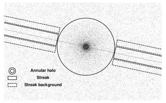
Figure 1: 2004 July 4 Chandra ACIS–S image (0.5–10 keV) of IGR J17544$-$2619. The image shows the presence of dust scattered halo as well as the ACIS readout streak. The inner radius of the annular halo is 5 arcsec, and the outer radius of the annular halo is 60 arcsec. The two pairs of boxes represent the streak area (solid) and the streak background area (dashed), respectively. Note that the width of the two pairs of boxes are enlarged (by a factor of 5) for clarity.

IGR J17544$-$2619 was observed with ACIS-S onboard Chandra X–ray Observatory on 2004 July 4 (ObsID 4550). The detector was operated in time exposure (TE) mode with a time resolution of 3.2 s, and the total exposure time is 19.06 ks. No grating spectroscopy was used. The position of IGR J17544$-$2619, ${\rm RA}=17^{\rm h}54^{\rm m}25\fs 284$, ${\rm Dec}=-26^{\circ}19\arcmin 52\farcs 62$ ($l=3\fdg 23$, $b=+0\fdg 33$, J2000), was reported by in’t Zand (2005). As shown in Figure 1, a diffuse X–ray halo is present with an extension of $\sim$60 arcsec around the point source. The data reduction is carried out with CIAO 4.5 and CALDB 4.5.6.

There are two prominent features in Figure 1: the pileup effect and the readout streak. Pileup means that within a single frame (typically, 3.2 s), at least two events occur at the same 3 pixel $\times$ 3 pixel island. The detected energy of these pileup events is approximately the sum of the individual ones. If the summed energy exceeds the onboard spacecraft threshold (i.e. 15 keV), it is rejected automatically by the built-in software of the spacecraft, probably leading to a visible “hole” in the image. In other cases, events can be so close to each other that their charge clouds overlap significantly, resulting in grade migration. Grade migration tends to spread charge into more than one pixel, degrading the quality of the event (Gaetz 2010), i.e., events with “good” ASCA grades (grade 0, 2, 3, 4, 6) might be converted into “bad” grades (grade 1, 5, 7). The presence of the readout streak is due to the fact that the Chandra ACIS detector system is shutterless. Hence, photons from the bright source can be detected while data in the CCD are being read out; thus the recorded events could have the same CHIPX as the bright point source, yet locate at any valid CHIPY.

2.1 Timing analysis

Due to the pileup effect, especially during the outburst, we extract the lightcurve of IGR J17544$-$2619 from the ACIS readout streak. Throughout this work we set the energy band to be $E\in(1,3)$ keV unless otherwise stated. The lower limit is chosen to be 1 keV because of the poor statistics of X–ray photons below 1 keV, and the upper limit is set to 3 keV due to the fact that the contribution of the dust scattered photons with higher energies are negligible, as the fractional halo intensity (relative to the source flux) is proportional to $E^{-2}_{\rm keV}$ (Smith et al., 2002). In addition, since the lightcurve is produced from streak data rather than on-axis data, correction of exposure time should be taken into consideration. The effective exposure time for the streak area ($T_{\rm str,exp}$) is

$$\small T_{\rm str,exp}=\frac{T_{\rm exp}}{T_{\rm frm}}\times N\times 0.00004~{}{\rm s},$$ (1)

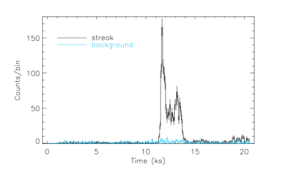
Figure 2: The 1–3 keV background subtracted lightcurve of IGR J17544$-$2619 (ObsID 4550). The lightcurve has been corrected with proper exposure time and the time bin is set to 100 s. The background level (blue), also corrected with proper exposure time, is presented as well.

where $T_{\rm exp}$ is the total exposure time of the observation, $T_{\rm frm}$ is the frame time, N is the number of rows in the streak area. After the correction of exposure time, the 1–3 keV background subtracted lightcurve of IGR J17544$-$2619 is shown in Figure 2. By setting a critical count rate of 0.1 cts s^-1, we divide the entire observation into the following three stages. The binary system is in the quiescent stage for the first $\sim 11.0$ ks with court rate $<$ 0.1 cts s^-1 (denoted as the pre-flare stage), then a strong flare occurs with a duration of $\sim 2.5$ ks (flare stage), and eventually it returns to the quiescent stage (post-flare stage).

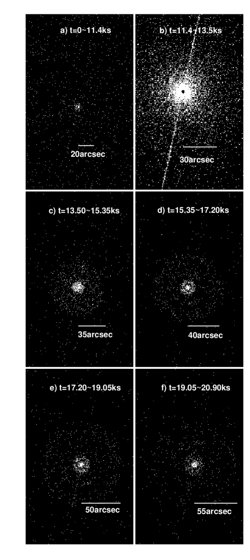
Figure 3: The time-dependent image of the expanding X–ray scattered halo around IGR J17544$-$2619. Panel a) the image of pre-flare stage with $t\in(0,11.4)$ ks; Panel b) the image of flare stage with $t\in(11.4,13.5)$ ks; Panel c-f) the images of post-flare stage with $t\in(11.3,20.9)$ ks.

The lightcurve is consistent with the time-dependent images of IGR J17544$-$2619 (Figure 3). The expanding X–ray scattered halo around IGR J17544$-$2619 is similar to those evolving X–ray scattered rings around GRBs (Vaughan et al., 2004, 2006; Tiengo & Mereghetti, 2006; Vianello et al., 2007) and magnetar bursts (Tiengo et al., 2010). However, we need to point out that the stacked images suffer from the contamination of the point spread function (PSF).

2.2 Imaging Analysis

2.2.1 Pileup estimation

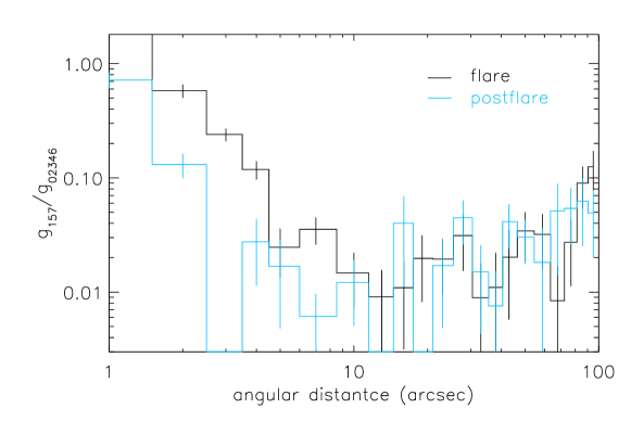
Figure 4: The 1–3 keV ASCA “bad/good” ratio, which can be served as a diagnostic of pileup effect. The black histogram is for the flare stage, while the blue one is for the post-flare stage.

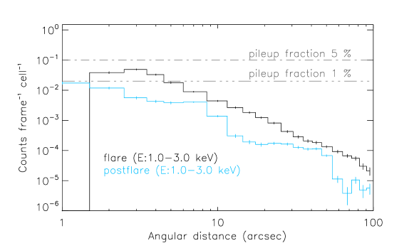
Figure 5: The 1–3 keV counts frame^-1 cell^-1 ratio as a function of angular distance for flare and post-flare stages, which can be served as a diagnostic of pileup effect. The horizontal dotted-dashed lines indicate a pileup fraction of 1% and 5%, respectively.

The interstellar dust in the vicinity of the point source, if any, might scatter the X–ray photons into small observation angles ($\lesssim 10$ arcsec). Therefore, we ought to estimate the pileup effect in order to acquire as much information as possible. The IGR J17544$-$2619 ObsID 4550 images the source on the back-illuminated (BI) chip ACIS-S3, for which, the $g_{0}/g_{6}$ criterion in estimating the pileup effect is not as effective as for the front-illuminated (FI) chips, because the background makes a significant contribution (Gaetz 2010). The “bad/good” ratio (Figure 4) in Level 1 event file can serve as a pileup indicator; the gradual rise of the “bad/good” ratio beyond $\theta\gtrsim 10~{}{\rm arcsec}$ is due the increasing importance of the background events with increasing radius (Gaetz 2010). Meanwhile, using the 3.2 s ACIS frame time and a Poisson-distributed count rate, we estimate the pileup effect via the same method adopted in Smith et al. (2002) and McCollough et al. (2013), i.e. a plot of counts frame^-1 cell^-1 as a function of radial distance for the flare and post-flare stage. The pre-flare stage is pileup free with the $E\in(1.0,3.0)$ keV count rate within a 2.5-arcsec-radius circle centered on the point source only $\sim 4.3\times 10^{-3}~{}{\rm cts}~{}{\rm s}^{-1}$. According to Davis (2007) , we take the counts frame^-1 cell^-1 values for which one would expect pileup fraction of 1% and 5% in Figure 5. According to both Figure 4 and Figure 5, for $\theta_{\rm obs}\in(4,60)$ arcsec, the pileup ($\lesssim 1\%$) barely affects the observation. Therefore, we can safely draw the inner boundary of the annular halo, i.e. the innermost 4.5 arcsec circular region is excluded in the following analysis. We set two groups of annular halos with different widths depending on the surface brightness: 1) the inner ones are 4.5–6.5 arcsec, 6.5–9.5 arcsec, and 9.5–12.5 arcsec; 2) the outer ones share the same width of 5 arcsec, with the median angular distance ranging from 15 arcsec to 60 arcsec.

2.2.2 The Radial profile

The radial profile of the Level 2 event file is created with the following main steps.

1. Generate the exposure map (in units of ${\rm ph}^{-1}~{}{\rm cts~{}s~{}cm^{2}}$) with the CIAO tool MKEXPMAP. Note that this exposure has taken the quantum efficiency (QE) and the effective area (ARF) into consideration.

2. Normalize the image (in units of ${\rm cts~{}pix^{-1}}$) by the exposure map with the CIAO tool DMIMGCALC. Now the obtained flux image ($F_{\rm img}$) is in units of ${\rm ph~{}s^{-1}~{}cm^{-2}~{}pix^{-1}}$.

3. Normalize the flux image with the source photon flux ($F_{\rm src}$, in units of ${\rm ph~{}s^{-1}~{}cm^{-2}}$) as follows:

   $$\small P=\frac{\sum_{A}F_{\rm img}}{F_{\rm src}\times A}~{}{\rm arcsec}^{-2}~{},$$ (2)

   where $A$ is the area (in units of ${\rm arcsec}^{2}$) of an annulus centered at the point source.

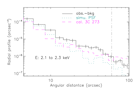
Figure 6: The difference between the background subtracted observational radial profile (black solid line) and simulated PSF radial profile (cyan dashed line) shows the existence of the X–ray scattered halo. The vertical dot-dashed line indicates that for $\theta\gtrsim 60~{}{\rm arcsec}$, the simulated PSF underestimates the wing of the genuine PSF. A background subtracted observational radial profile of a calibration observation (toward 3C 273) is used for the PSF radial profile at $\theta\gtrsim 60~{}{\rm arcsec}$ instead.

Likewise, the radial profile of the PSF can also be obtained. The PSF event file could be simulated with ChaRT and MARX, while the exposure map and the photon flux are the same as those for the Level 2 event file. The difference between the background subtracted observational radial profile and the PSF radial profile shows the existence of the X–ray scattered halo (Figure 6). As pointed out by Smith et al. (2002), the simulated PSF underestimates the wing of the genuine PSF. Therefore, a background subtracted observational radial profile of a calibration observation toward 3C 273 (ObsID 14455) is used at $\theta\gtrsim 60~{}{\rm arcsec}$ instead. Since 3C 273 is located at high galactic latitude ($b=+64\fdg 36$, J2000) and has a low LOS hydrogen column density of $\sim 1.7\times 10^{20}~{}{\rm cm}^{-2}$, we believe the contribution of X-ray scattered halo in the radial profile is negligible.

We should be aware that, in our case, the radial profile in Figure 6 underestimates the contribution of the dust scattered halo for two main reasons. (1) Due to the transient nature of IGR J17544$-$2619, the dust scattered halo photons are not always there; however, the exposure time for the entire observation is used in the denominator, since we do not know the exact exposure time for the halo photons at a certain angular distance. (2) The photon flux of IGR J17544$-$2619 is obtained by fitting the spectrum with the absorbed power law model for the entire observation; however, the photon flux of the flare stage is about three orders of magnitude greater than that of the quiescent stage (see Table 1 in Rampy et al. (2009)). Unfortunately, the effective area of Chandra is so small that we fail to have sufficient statistics in the quiescent stage for detailed spectral analysis.

Therefore, the overestimation of both the exposure time and the source photon flux lead to the underestimation of the contribution of the dust scattered halo in the radial profile. Similarly, we also cannot calculate the fractional halo intensity (FHI; see the definition in Mathis & Lee (1991); Xiang et al. (2005)), since the halo is time-dependent. Thus the definition of FHI works well for persistent systems, but not very meaningful in terms of the dust scattered halo caused by prompt emission (e.g. flares of the SFXTs or GRBs).

3 Distance Measurement

3.1 Cross correlation function

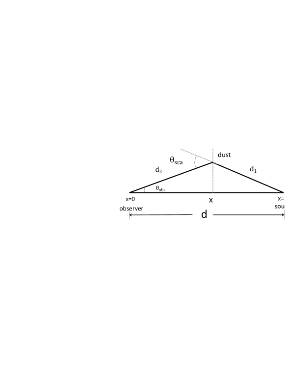
Figure 7: A sketch of small angle X–ray scattering.

As shown in Figure 7, the scattered photons travel longer paths than the unscattered ones ($d_{1}+d_{2}>d$), hence it is reasonable to expect time lags of the flare arrival time in the dust scattered halo lightcurves. Here we use the cross correlation method (Ling et al., 2009b) to determine the delay times of the scattered halo photons. We cross correlate the background subtracted streak lightcurve with each background subtracted annular halo lightcurve. The cross correlation function (CCF) is given as follows:

$$\small{c}(\tau)=\frac{1}{N-|\tau|}\sum_{t=0}^{N-|\tau|-1}\frac{({L}_{\rm h}({t}+\tau)-\overline{L}_{\rm h})}{\sigma_{\rm h}}\frac{({L}_{\rm s}({t})-\overline{L}_{\rm s})}{\sigma_{\rm s}},$$ (3)

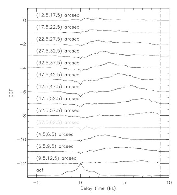
Figure 8: The Auto correlation function subtracted cross correlation functions between the streak lightcurve and each of the background subtracted observed halo lightcurve. The vertical dot–dashed line indicate the end of the observation. For clarity, all but the first CCFs have been lowered by 1.0 successively.

where ${c}(\tau)$ is the cross correlation coefficient, $\tau$ is the delay time, $N$ is the total number of time bins, $L_{X}$ is the lightcurve of annular halo ($X=h$) or streak ($X=s$), $\overline{L}_{X}$ and $\sigma_{X}$ are the corresponding mean value and standard deviation, respectively. Subsequently, we subtract the auto correlation function (ACF) of the streak lightcurve, and show the results in Figure 8. We conservatively subtract the ACF of the streak lightcurve rather than subtract the contamination of the PSF contribution in each annular halo lightcurve, mainly because there are some uncertainties in the estimation of the PSF contribution. For instance, as shown in the 2.1–2.3 keV halo profile (Figure 6), the simulated PSF under-estimates the genuine one at larger angular distances, so that the PSF fractions obtained from the PSF event file could be biased. On the other hand, the count rate of the point source estimated via the count rate of the streak area also has uncertainty. Apparently, there are two distinct groups of CCFs shown in Figure 8. For annular halos with $\theta_{\rm obs}\in(12.5,57.5)$ arcsec, the peaks of CCFs show a clear trend of a shift to the right. Unfortunately, the peak of the CCF of the halo at $\theta_{\rm obs}=60$ arcsec, if any, moves out of the end of the this observation (vertical dot–dashed line at the right in Figure 8). On the other hand, the CCFs for the inner three halos with $\theta_{\rm obs}\in(4.5,6.5)$ arcsec, $\theta_{\rm obs}\in(6.5,9.5)$ arcsec and $\theta_{\rm obs}\in(9.0,12.5)$ arcsec present relatively longer delay times.

Since the errors of the CCFs obtained above are unavailable analytically, we turn to Monte Carlo simulations. Sampled photon counts in each time bin of the lightcurves is generated either from normal distributions with the mean values set to net photon counts or from Poisson distributions with the values of $\lambda-$parameters equal to the net photon counts. Note that for the majority of those bins which contribute mostly to the peaks of the CCFs, sufficient counts ($\gtrsim 10$) are guaranteed as we choose the width of each annuli to meet such kind of requirement. Hence it is reasonable to simply adopt normal distributions here, although the errors given by normal distributions are smaller than that of Poisson distributions. In terms of locating the peaks of the CCFs, again we use two different methods. One is to fit the $\pm 23$ data points centered at the peak of each CCF with an individual Gaussian function during each realization, and then determine the mean time delay and the standard deviation for the time lags for each annular halo. Alternatively, we simply find the point which yields the maximum value of the CCF during each realization, and then calculate the mean values and the standard deviations. The mean time lags and errors obtained after $10^{3}$ Monte Carlo realisations are reported in Table 1. Note that the uncertainty in this work for each parameter is given at 68.3% confidence level, unless otherwise indicated. Apparently, both the peak values and the numbers of invalid Gaussian fit suggest that the time lags of the three annular halos (12.5–17.5 arcsec, 17.5–22.5 arcsec and 22.5–27.5 arcsec) are less reliable. However, the time lags yielded by the four data sets (Norm./Poi.+Gau./Max.) of the remaining five annular halos with $\theta\in(27.5,57.5)$ arcsec agree within $1\sigma$ uncertainty level.

3.2 $\theta_{\rm ari}$ and $\theta_{\rm ave}$

In practice, we extract halo lightcurves from wide concentric annuli around the point source in order to have sufficient counts, and simply assign the median angular distance $\theta_{\rm mid}=(\theta_{\rm obs,e}+\theta_{\rm obs,i})/2$ as the $\theta_{\rm obs}$ for each annulus, where $\theta_{\rm obs,e}$ and $\theta_{\rm obs,i}$ are the exterior and interior boundaries of annular regions, respectively. However, $\theta_{\rm mid}$ could deviate from $\theta_{\rm obs}$ significantly, due to sharply and nonlinearly decreasing scattering cross section as a function of $\theta_{\rm obs}$. Particularly, for those halos caused by the dust located in the vicinity of the point source, the differential scattering cross section ${d\sigma_{\rm sca}}/{d\Omega}$ declines non-linearly with the increasing scattering angle $\theta_{\rm sca}$, where $\theta_{\rm sca}=\theta_{\rm obs}/(1-x)$ (Mathis & Lee, 1991) holds for small observational angles. The deviation in delay time caused by $\Delta\theta=\theta_{\rm obs}-\theta_{\rm mid}$ is

$$\Delta t_{\rm dly}=2.42\times 10^{-3}\left(\frac{x}{1-x}\right)\left(\frac{d}{\rm kpc}\right)\left(\frac{\theta\Delta\theta}{{\rm arcsec}^{2}}\right)~{}{\rm ks}.$$ (4)

For instance, assuming $\theta_{\rm obs}=10$ arcsec, $\Delta\theta_{\rm obs}=1$ arcsec and $d=4$ kpc, for $x\leqslant 0.500$, we have $\frac{x}{1-x}\leqslant 1.0$, and thus $\Delta t_{\rm dly}\leqslant 0.1$ ks. For $x\geqslant 0.909$, however, $\frac{x}{1-x}\geqslant 10.0$, and thus $\Delta t_{\rm dly}\geqslant 1$ ks, which is comparable to the observed total delay time. Therefore, when the dust slab is in the vicinity of the point source, it is important to model $\theta_{\rm obs}$ properly when determining the delay times of the scattered halo photons.

We extract the observed halo photons with $E\in(2.0,3.0)$ keV and $t_{\rm arr}=t_{\rm pk}+t_{\rm dly}\pm t_{\rm dly,err}$ for the three annular regions, where $t_{\rm arr}$ is the arrival time of the halo photons, $t_{\rm pk}$ is the time when the streak lightcurve (used as a proxy for the source lightcurve) reaches its maximum, $t_{\rm dly}$ and $t_{\rm dly,err}$ are listed in Table 1. The time intervals are set so that the dust scattered halo photons (net counts) dominates the PSF photons and the background photons out there. In fact, the background counts ($\lesssim 10^{-1}$) are negligible here. While for the PSF photons, we run ChaRT and MARX to simulate the observation and generate $\sim 10^{3}$ PSF photons within each of the three annuli. We subtract the contribution from the PSF photons, and then list in Table 2 the arithmetic mean angular distance of each annulus,

$$\theta_{\rm ari}=\frac{1}{N}~{}\sum_{i}\theta_{i},$$ (5)

where $\theta_{i}$ is the angular distance of the $i$th photon and $N$ is the total number of photons in this annulus, respectively. Apparently, when the dust slab is close to the point source, $\theta_{\rm ari}$ does differ from $\theta_{\rm mid}$.

To be more specific, we can calculate the single-scattering cross section with Rayleigh-Gans (RG) approximation of the differential scattering cross section (Mathis & Lee, 1991)

$$\frac{d\sigma_{\rm sca}}{d\Omega} = c_{1}\left(\frac{2Z}{M}\right)^{2}\left(\frac{\rho}{{\rm 3\ g\ cm}^{-3}}\right)^{2}\left(\frac{a}{\mu\rm{\ m}}\right)^{6}$$ (6)

$$\times\left[\frac{F(E)}{Z}\right]^{2}{\rm exp}\left(-K^{2}\left(\frac{\theta_{\rm sca}}{\rm arcmin}\right)^{2}\right)~{},$$

where $c_{1}=9.31\times 10^{-8}~{}{\rm cm}^{2}{\rm arcmin}^{-2}$, $Z$ is the mean atomic charge, $M$ is the molecular weight (in units of amu), $\rho$ is the mass density, $F(E)$ is the atomic scattering factor, and $K^{2}=0.4575(E/{\rm keV})^{2}(a/{\mu{\rm m}})^{2}$. As pointed out by Smith & Dwek (1998), the RG approximation fails for incident photons with energies $E\lesssim 2$ keV. Hence, in the following analysis we only focus on photons with $E\gtrsim 2$ keV. With one thin dust slab located at $x=x_{i}$ along the LOS, the single-scattering cross section at $\theta_{\rm obs}$ is

$$\sigma_{\rm sca}(x=x_{i},\theta_{\rm obs}) = \int S(E)dE\int f(x_{i})N_{\rm H}n(a)$$ (7)

$$\times\frac{d\sigma_{\rm sca}}{d\Omega}(a,E,\theta_{\rm obs},x_{i})da~{},$$

where $S(E)$ is the normalized photon energy distribution, $n(a)$ is the dust size distribution (in units of particles per H atom per micron), $f(x_{i})$ is the density of hydrogen at $x\cdot d$ relative to the average hydrogen column density along the LOS to IGR J17544$-$2619 and here we set $f(x_{i})$ to unity. For simplicity, Equation 7 is substituted with

$$\sigma_{\rm sca}(x=x_{i},\theta_{obs}) = \sum_{k=0}^{9}n(E_{k})\int f(x_{i})N_{\rm H}n(a)$$

$$\times\frac{d\sigma_{\rm sca}}{d\Omega}(E_{i},a,\theta_{\rm obs},x_{i})da~{},$$

where $n(E_{k})$ is the normalized observed spectrum within the range of $E\in(E_{k}-0.05,E_{k}+0.05)$ keV, $E_{k}=(2.05+0.1k)$ keV, and $\sum n(E_{k})=1$. We obtain the average observational angles ($\theta_{\rm ave}$) predicted by MRN, WD01, ZDA and XLNW dust models via

$$\theta_{\rm ave}=\frac{\int\frac{d\sigma_{\rm sca}}{d\Omega}(x=x_{i},\theta_{\rm obs})\theta_{\rm obs}^{2}d\theta_{\rm obs}}{\int\frac{d\sigma_{\rm sca}}{d\Omega}(x=x_{i},\theta_{\rm obs})\theta_{\rm obs}d\theta_{\rm obs}}~{}.$$ (8)

An advantage of Equation 8 is that $\theta_{\rm ave}$ does not depend on the distance of the point source. Consequently, we can break the degeneracy between the distances of the point source and the dust slab in Equation 9.

3.3 Distance measurement

The relationship between the delay time and geometrical distances of interstellar dust and the point source is given by Trümper & Schönfelder (1973),

$$\left(\frac{t_{\rm dly}}{\rm ks}\right)=1.21\times 10^{-3}\frac{x}{1-x}\left(\frac{d}{\rm kpc}\right)\left(\frac{\theta_{\rm obs}}{\rm arcsec}\right)^{2},$$ (9)

where $x$ is the normalized distance of the dust cloud, $d$ is the distance of the point source, $\theta_{\rm obs}$ is the observational angle of the halo photons and here we simply assign $\theta_{\rm obs}=\theta_{\rm mid}$. In fact, Rahoui et al. (2008) reported a distance of 3.6 kpc for IGR J17544$-$2619 using mid-infrared photometry and spectroscopy. The result is within the range $d\in(2.1,4.2)$ kpc given by Pellizza et al. (2006).

We first adopt a distance of 3.6 kpc for IGR J17544$-$2619 and fit the delay times for the halos caused by the closer dust to determine the normalized dust distance ($x$); the results are listed in Table 3. Note that for those fits with reduced chi-squared values greater than 3, we only report values of $x$ yielding the smallest reduced chi-squared values. The results obtained from the four sets of data are consistent with each other within the 68.3% confidence level. In terms of the halos caused by the farther dust, the reduced chi-squared values are significantly greater than unity, so that the normalized distances of the farther dust cloud are less reliable. Simply by solving Equation (9) with the three time lags of the Poi.+Max. data, we have three normalized dust distances, $0.952^{+0.004}_{-0.005}$ for $\theta_{\rm obs}\in(4.5,6.5)$ arcsec, $0.944^{+0.004}_{-0.004}$ for $\theta_{\rm obs}\in(6.5,9.5)$ arcsec and $0.925^{+0.006}_{-0.008}$ for $\theta_{\rm obs}\in(9.5,12.5)$ arcsec, which indicates that the farther dust could probably be a complex or a giant molecular cloud; alternatively, the simple model needs to be modified.

Since no uncertainty of the point source distance was reported in Rahoui et al. (2008), here we attempt to do distance measurement via the X-ray scattered halo. Since the two parameters $x$ and $d$ in Equation (9) are highly degenerated and negatively correlated, we introduce a parameter called distance factor

$$\mathscr{D}=\frac{x}{1-x}\frac{d}{\rm kpc},$$ (10)

which contains information of dust distance and source distance and can be determined with the delay time of the scattered halo photons. Substituting $\mathscr{D}$ into Equation (9), we have

$$\left(\frac{t_{\rm dly}}{\rm ks}\right)=1.21\times 10^{-3}\mathscr{D}\left(\frac{\theta_{\rm obs}}{\rm arcsec}\right)^{2}~{}.$$ (11)

The results for $\mathscr{D}$ are listed in Table 4. Apparently, for the closer dust cloud, $\mathscr{D}$ could be well constrained for the Norm./Poi.+Max. data sets; whereas for the farther dust cloud, the values of $\mathscr{D}$ fail to agree for all four data sets. Moreover, using $\theta_{\rm ari}$ instead of $\theta_{\rm mid}$ when fitting data with Equation (11) cannot eliminate the discrepancy. The inconsistency is mainly due to the fact that even a small deviation in $x$ ($\Delta x\sim 0.01$) could lead to a substantial change in $\mathscr{D}$ with $\Delta\mathscr{D}\sim 10$.

In order to determine the point source distance ($d$), we need to firstly obtain the normalized distance of the dust ($x$) by comparing the arithmetic mean values ($\theta_{\rm ari}$) of the observed scattered halo photons within different annular regions with the average mean values ($\theta_{\rm ave}$) calculated with dust grain models. Meanwhile, the time lags of the scattered halo photons obtained through the cross correlation method and $\theta_{\rm ari}$ allow us to determine $\mathscr{D}$, which is a function of both $d$ and $x$. Substituting $x$ into Equation (10), $d$ is derived finally.

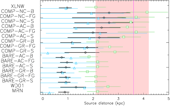
Figure 9: The distances of IGR J17544$-$2619 determined with different dust grain models. The black diamond, blue triangles and green squares indicate the results obtained with $\theta\in(27.5,52.5)$ arcsec, $\theta\in(6.5,9.5)$ arcsec and $\theta\in(4.5,12.5)$ arcsec annular halos, respectively. The pink region and solid magenta line show the results of the two IR observations.

To be more specific, for the inner three individual annular halos (4.5–6.5 arcsec, 6.5–9.5 arcsec and 9.5–12.5 arcsec) caused by the farther dust, by varying $x\in(0.900,0.999)$ with step $\Delta x=0.001$, we find the minimum values of $|\theta_{\rm ave}-\theta_{\rm ari}|$ (for $E\in(2.0,3.0)$ keV) and the best $x$. Unfortunately, due to the low counts, the uncertainty of $\theta_{\rm ari}$ is rather large. Consequently, even the derived $x$ of the 6.5–9.5 arcsec annular halo, which has the smallest uncertainty on $\theta_{\rm ari}$, can barely constrain $d$ (see the blue triangles in Figure 9).

Alternatively, we use the combination of the individual annular halos caused by the farther dust cloud. Due to the sufficient counts within $\theta\in(4.5,12.5)$ arcsec $x$ can be well constrained (Table 5). As for $\mathscr{D}$, we simply set,

$$\mathscr{D}=\frac{1}{3}{\sum_{i=0}^{2}\mathscr{D}_{i}}~{},\delta\mathscr{D}=\sqrt{\sum_{i=0}^{2}\delta\mathscr{D}_{i}^{2}}~{}.$$ (12)

Due to the large uncertainty in $\mathscr{D}$, the source distance cannot be narrowly constrained.

On the other hand, in terms of the annular halos caused by the closer dust cloud, we combine the four annular halos with $\theta\in(27.5,52.5)$ arcsec, and vary $x\in(0.20,0.90)$ with step $\Delta x=0.01$ to search for the minimum values of $|\theta_{\rm ave}-\theta_{\rm ari}|$ and the best $x$. $\mathscr{D}$ is well constrained via the cross correlation method for the closer dust. However, the uncertainty in $x$ is quite large due to the relatively low counts in such a wide region. Thus, the source distance cannot be well constrained neither (see also Table 5).

Not all of the point source distances derived above are reasonable when compared to the results obtained with IR observations (Pellizza et al., 2006; Rahoui et al., 2008). Figure 9 illustrates the source distances obtained with different dust grain models. Given the distance range $d\in(2.1,4.2)$ kpc (Pellizza et al., 2006), it seems that four dust grain models COMP-AC-S/B, COMP-NC-S/FG (labeled with $\surd$ in Table 5) are better, since both $d_{1}$ and $d_{2}$ are within the distance range, i.e. $d_{i}\in(2.1,4.2)~{}{\rm kpc},i=1~{}{\rm and}~{}2$. COMP-GR-S/FG, COMP-AC-FG, COMP-NC-B (labeled with $\bigcirc$) are also acceptable, since either $d_{1}$ or $d_{2}$ is within the distance range, while the other is consistent with the distance range within $1\sigma$ error, i.e. $|d_{\rm b}-d_{i}|\in d_{i,\rm err},i=1~{}{\rm or}~{}2$, where the upper and lower boundary of the distance range $d_{\rm b}=2.1~{}{\rm and}~{}4.2$ kpc, respectively. However, for the rest of the dust grain models, $d_{1}$ is within the distance range or consistent within 1$\sigma$ uncertainties (BARE-GR/AC-B), while $d_{2}$ is inconsistent with the distance range within 1$\sigma$ uncertainties ($|2.1-d_{2}|>d_{2,\rm err}$).

4 Discussion

4.1 Kinematic distance measurements of molecular clouds

For $d\sim 3.6$ kpc (Rahoui et al., 2008), the distances for the closer and farther dusts are $\sim 1.8$ kpc and $\sim 3.4$ kpc away from us, respectively. In this subsection we try to find kinematic distance measurements of the molecular clouds along the LOS toward IGR J17544$-$2619  for comparison with our geometrical distances of the dust slabs. A rough estimate of the radial velocity of the molecular clouds where the dust slab is embedded can be made via (Roman-Duval et al., 2009)

$$r=R_{\odot}\sin l\frac{V(r)}{v_{\rm los}+V_{\odot}\sin l},$$ (13)

where $r$ is the distance of the molecular cloud to the Galactic Center (GC), $R_{\odot}$ is the distance of the Sun to GC, l is the galactic longitude of the LOS, $V_{\odot}$ is the rotation velocity of the Sun, $V(r)$ is the rotation velocity of the molecular cloud, and $v_{\rm los}$ is the projection of $V(r)$ to the LOS, also known as the radial velocity. Assuming $R_{\odot}=8.5$ kpc, $V_{\odot}=220$ km s^-1 and a flat rotation curve (i.e. $V(r)=220$ km s^-1), we derive $v_{\rm los}$ of $\sim 3.1$ km s^-1 and $\sim 7.8$ km s^-1 for the closer and farther molecular cloud, respectively. In fact, Dahmen et al. (1998) reported an averaged $v_{\rm los}\sim 5$ km s^-1 for ¹²CO(1-0) emission line for the Southern Clump 2 region, $l\in(2\fdg 7,3\fdg 5)$, $b\in(0\fdg 15,0\fdg 35)$, which is roughly consistent with our result of the farther dust.

4.2 Issues with observational angles

In Section 3.2, we have shown that given the normalized distance of a dust slab, different interstellar dust models predict different average observational angles for scattered photons within certain annular regions. This offers the advantage of estimating the parameter $x$ from data, thus breaking the degeneracy between $x$ and $d$. We tested several interstellar dust grain models with the data of the farther dust, for which the predictions of these models become quite different, because the scattering angle $\theta_{\rm sca}=\theta_{\rm obs}/(1-x)$ is quite large for the farther dust. It is therefore possible to distinguish among different interstellar dust models, as demonstrated above. However in the calculations of the scattering differential cross section, Gaussian approximation is used for the form factor in the RG approximation. Smith & Dwek (1998) pointed out that the Gaussian approximation leads to deviations at large scattering angle ($\gtrsim 200~{}{\rm arcsec}$) and large dust grain size. In our case, i.e., $x>0.95$ and $\theta_{\rm obs}\sim 10~{}{\rm arcsec}$ for the farther dust slab, we have $\theta_{\rm sca}>200$ arcsec. Moreover, the upper limits of the grain size are greater than 0.3 micron, and even reach to 0.9 micron. Therefore the Gaussian approximation may cause considerable inaccuracies to the model predictions. Alternatively, one can turn to Mie theory (van de Hulst, 1957), which is more accurate for $E\sim 1~{}$keV and/or large scattering angles, but numerically more difficult to carry out the calculations.

5 Summary

In this work, we analyzed the X–ray scattered halo around IGR J17544$-$2619 with cross correlation method. The main results are summarized as follows:

1. From the cross correlation functions between the streak lightcurve (used as a proxy for the point source lightcurve) and the lightcurves of the annular halos, we conclude that there are at two interstellar dust clouds along the LOS toward IGR J17544$-$2619.

2. By comparing the observational angle of the scattered halo photons with that predicted by different dust grain models, the normalized dust distance can be determined independent of the distance of the point source.

3. Given the point source distance of $\sim 3.6$ kpc, the closer dust, which is $\sim 1.8$ kpc away from us, is responsible for X–ray scattered halos at larger observational angles ($\gtrsim 12.5$ arcsec). The farther dust, which is quite close to the point source ($\sim 3.4$ kpc away from us), explains the X–ray scattered halos at smaller angular distances ($\lesssim 12.5$ arcsec).

4. We determined the model-dependent point source distances, which are compared with that yielded by IR observations. We find that among the 18 tested dust grain models (MRN, WD01, ZDAs and XLNW), the four dust grain models COMP-AC-S/B, COMP-NC-S/FG are better, COMP-GR-S/FG, COMP-AC-FG, COMP-NC-B are also acceptable, but the rest dust grain models fail to obtain consistent source distance.

Similar to the GRBs, the transient nature of SFXTs can, in principle, be used to precisely determine the geometrical distances of interstellar dust and the point source by taking advantage of the time delay effect of the small angle X–ray scattering phenomena. However, we have to face some practical difficulties, such as: 1) the angular resolutions of the space telescopes are relatively poor; 2) the effective area is small and thus the photon counts are relatively low; or 3) for observations of X–ray scattered halo caused by dust slab in the vicinity of the point source, the time lags can be quite large, but no observations with sufficiently long effective exposure times are available. The effective exposure time refers to the exposure time for observing the X–ray scattered halo. For instance, in our work, since the outburst occurs $\sim$ 10 ks after the beginning of this observation, the effective exposure time for observing the X–ray scattered halo here is only $\sim$ 9 ks.

With the fine angular resolution, Chandra has the capability to observe X–ray scattered halos around SFXTs especially at smaller angular distance, although the collecting area of ACIS is small. Unfortunately, insofar as the archival Chandra data, only IGR J17544$-$2619 (ObsID 4550) allows us to study the X–ray scattered halo. In terms of other observations of SFXTs, either the exposure time is only several kiloseconds (e.g. XTE J1739$-302$), or no flaring activity was caught (e.g., for IGR J19410$-$0951). Therefore, we suggest that in the future more long term follow up observations of the outbursts of SFXTs shall be made with Chandra to study the X–ray scattered halo and thus the interstellar dust models in further details.

Appendix A Thick Dust Layer

The smallest size of the giant molecular clouds (GMCs) in the Milky Way has been found to be 5 pc (Murray, 2011). Therefore the farther dust cloud located $\lesssim 100$ pc away from the binary system is no longer “thin” when compared to the distance between the cloud and the point source. Consequently, the validity of the treatment of the dust cloud as a “thin” slab should be examined. Consider a point source at a distance of 2 kpc along with a “thick” dust cloud with a thickness of 10 pc located at$x\gtrsim 0.90$), the dust scattering cross section of such a cloud can be calculated as the sum of five ($N=5$) “thin” slabs

$$\sigma_{\rm thick}=\sum_{i=0}^{4}~{}\int S(E)dE\int\frac{N_{\rm H}}{N}n(a)\times\frac{d\sigma_{\rm sca}}{d\Omega}(a,E,\theta_{\rm obs},x_{i}=x_{0}+i\times\Delta x)da.$$ (A1)

For simplicity, we assume a mono-energy spectrum ($E=2$ keV) and $\theta_{\rm obs}=10$ arcsec. We compare $\sigma_{\rm thick}$ with the cross section of a single “thin” dust slab located at $x=\bar{x}_{i}$, which has a thickness of 2 pc and the same total column density as that of the “thick” cloud, by calculating

$$R=\frac{\frac{1}{N}\sum_{i=0}^{4}\int n(a)\times\frac{d\sigma_{\rm sca}}{d\Omega}(a,E,\theta_{\rm obs},x_{i}=x_{0}+i\times\Delta x)da}{\int n(a)\times\frac{d\sigma_{\rm sca}}{d\Omega}(a,E,\theta_{\rm obs},x_{i}=\bar{x})da}$$ (A2)

for four typical dust grain models (MRN, WD01, XLNW and ZDA COMP-GR-S) with $\bar{x}=0.900,~{}0.950~{}{\rm and}~{}0.990$ (Table 6), respectively. Note that the XLNW model is a modified form of ZDA BARE-GR-S model (Xiang et al., 2011). Clearly in all cases $R$ does not deviates from unity significantly, indicating that the “thin” dust cloud assumption is a good approximation when $x\lesssim 0.990$ and the size of the dust cloud is not significantly large ($\lesssim 10~{}$pc).

Table 1: Time lags of the annular halos.

$\theta_{\rm obs}$	Norm.+Gau.		Norm.+Max.		Poi.+Gau.		Poi.+Max.
arcsec	$t_{\rm dly}$ (ks)	C${}_{\rm max}^{\rm a}$ ($n^{\rm b}$)	$t_{\rm dly}$ (ks)	Cmax	$t_{\rm dly}$ (ks)	C${}_{\rm max}(n)$	$t_{\rm dly}$ (ks)	Cmax
12.5-17.5	$2.84\pm 0.09$	0.00 (997)	$0.95\pm 0.64$	0.18	$2.72\pm 0.92$	0.00 (977)	$1.10\pm 0.72$	0.17
17.5-22.5	$2.88\pm 0.37$	0.01 (892)	$1.46\pm 0.44$	0.22	$3.03\pm 0.37$	0.03 (797)	$1.59\pm 0.58$	0.22
22.5-27.5	$2.82\pm 0.40$	0.13 (327)	$1.99\pm 0.53$	0.30	$2.89\pm 0.49$	0.16 (175)	$2.08\pm 0.64$	0.30
27.5-32.5	$3.04\pm 0.15$	0.24 (209)	$2.50\pm 0.24$	0.39	$3.02\pm 0.13$	0.29 (61)	$2.48\pm 0.20$	0.40
32.5-37.5	$3.50\pm 0.12$	0.35 (13)	$3.24\pm 0.12$	0.44	$3.50\pm 0.10$	0.36 (2)	$3.23\pm 0.11$	0.45
37.5-42.5	$4.64\pm 0.12$	0.46 (1)	$4.37\pm 0.26$	0.50	$4.66\pm 0.10$	0.47 (0)	$4.37\pm 0.25$	0.50
42.5-47.5	$5.60\pm 0.13$	0.46 (0)	$5.72\pm 0.19$	0.50	$5.53\pm 0.11$	0.45 (0)	$5.70\pm 0.19$	0.50
47.5-52.5	$6.71\pm 0.20$	0.35 (32)	$6.99\pm 0.43$	0.41	$6.64\pm 0.17$	0.36 (4)	$6.88\pm 0.40$	0.41
52.5-57.5	$7.59\pm 0.42$	0.14 (428)	$7.99\pm 0.37$	0.28	$7.56\pm 0.54$	0.23 (35)	$7.81\pm 0.45$	0.27
57.5-62.5	$-1.88\pm 7.42$	0.00 (989)	$0.90\pm 3.51$	0.10	$-7.27\pm 3.66$	0.16 (846)	$-0.55\pm 4.16$	0.12
4.5-6.5	$3.06\pm 0.13$	0.33 (43)	$2.60\pm 0.30$	0.38	$3.08\pm 0.12$	0.34 (22)	$2.63\pm 0.27$	0.39
6.5-9.5	$4.70\pm 0.23$	0.35 (1)	$4.66\pm 0.38$	0.35	$4.79\pm 0.20$	0.36 (0)	$4.70\pm 0.34$	0.37
9.5-12.5	$6.33\pm 0.36$	0.20 (30)	$6.57\pm 0.99$	0.23	$6.09\pm 0.34$	0.21 (2)	$6.48\pm 0.63$	0.24

Note. — “Norm.”: the sampled photon counts generated from normal distributions; “Poi.”: the sampled photon counts generated from Poisson distributions; “Gau.”: an individual Gaussian function is used to fit the nearby data points centered at the peak of each CCF; “Max.”: the maximum value of the CCF is used.

Table 2: $\theta_{\rm ari}$ and distance factor ($\mathscr{D}$) for scattered halo photons with $E\in(2.0,3.0)$ keV.

annuli (arcsec)	(4.5, 6.5)	(6.5, 9.5)	(9.5, 12.5)	(4.5, 12.5)	(27.5, 52.5)
$t_{\rm arr}~{}(\rm ks)$	(14.0, 14.6)	(16.0, 16.7)	(17.5, 18.8)	(12.5, 19.1)	(12.5, 19.1)
number of net counts	18.86	40.51	33.19	347.45	288.24
$\theta_{\rm ari}$ (arcsec)	$5.25\pm 0.14$	$7.76\pm 0.14$	$10.63\pm 0.17$	$7.56\pm 0.11$	$39.79\pm 0.42$
$\mathscr{D}$	$78.91\pm 9.16^{\rm a}$	$64.67\pm 5.18^{\rm a}$	$47.40\pm 4.86^{\rm a}$	$63.66\pm 11.59^{\rm b}$	$2.24\pm 0.07^{\rm c}$

Table 3: The normalized distances ($x$) of dust with source distance ($d$) fixed to 3.6 kpc.

	Norm.+Gau.	Norm.+Max.	Poi.+Gau.	Poi.+Max.
$\chi^{2}$/d.o.f.	20.9/5	3.7/8	27.5/5	4.5/8
$x$ for (12.5, 57.5) arcsec	$0.52$	$0.518\pm 0.005$	$0.52$	$0.517\pm 0.005$
$\chi^{2}$/d.o.f.	88.8/2	6.5/2	115.8/2	13.1/2
$x$ for (4.5, 12.5) arcsec	$0.96$	$0.96$	$0.96$	$0.96$

Table 4: Determining the distance factor $\mathscr{D}$ by fitting the time lags with Equation (11).

$\theta_{\rm obs}$ (arcsec)	para.	Norm.+Gau.	Norm.+Max.	Poi.+Gau.	Poi.+Max.
(12.5, 57.5)	$\chi^{2}$/d.o.f.	20.9/5	3.7/8	27.5/5	4.5/8
with $\theta_{\rm mid}$	$\mathscr{D}$	$2.3$	$2.26\pm 0.04$	$2.3$	$2.24\pm 0.07$
(4.5, 12.5)	$\chi^{2}$/d.o.f.	88.8/2	6.5/2	115.7/2	13.1/2
with $\theta_{\rm mid}$	$\mathscr{D}$	$57.7$	$58.0$	$57.9$	$55.2$
(4.5, 12.5)	$\chi^{2}$/d.o.f.	91.6/2	6.6/2	118.6/2	13.0/2
with $\theta_{\rm ari}$	$\mathscr{D}$	$62.3$	$62.3$	$62.5$	$59.9$

Table 5: Differences between $\theta_{\rm ari}$ and $\theta_{\rm ave}$ and distances $x$ and $d$.

No.	Model Name	$(\theta_{\rm ave}-\theta_{\rm ari})_{1}$	$x_{1}^{\rm a}$	$d_{1}^{\rm b}$	$(\theta_{\rm ave}-\theta_{\rm ari})_{2}$	$x_{2}^{\rm a}$	$d_{2}^{\rm b}$	Acpt.
		arcsec		kpc	arcsec		kpc
01	MRN	0.008	$0.967^{+0.002}_{-0.002}$	$2.17^{+0.42}_{-0.42}$	0.009	$0.72^{+0.04}_{-0.06}$	$0.87^{+0.17}_{-0.26}$
02	WD01	0.007	$0.961^{+0.003}_{-0.003}$	$2.58^{+0.51}_{-0.51}$	0.002	$0.63^{+0.07}_{-0.11}$	$1.32^{+0.40}_{-0.62}$
03	BARE-GR-S	-0.009	$0.968^{+0.002}_{-0.003}$	$2.10^{+0.40}_{-0.43}$	-0.027	$0.71^{+0.04}_{-0.07}$	$0.91^{+0.18}_{-0.31}$
04	BARE-GR-FG	-0.004	$0.968^{+0.003}_{-0.002}$	$2.10^{+0.40}_{-0.43}$	0.008	$0.71^{+0.04}_{-0.06}$	$0.91^{+0.18}_{-0.26}$
05	BARE-GR-B	0.019	$0.973^{+0.003}_{-0.002}$	$1.77^{+0.38}_{-0.35}$	0.032	$0.75^{+0.04}_{-0.05}$	$0.75^{+0.16}_{-0.20}$
06	BARE-AC-S	0.004	$0.967^{+0.003}_{-0.003}$	$2.17^{+0.44}_{-0.44}$	-0.039	$0.71^{+0.04}_{-0.07}$	$0.91^{+0.18}_{-0.31}$
07	BARE-AC-FG	-0.009	$0.967^{+0.002}_{-0.003}$	$2.17^{+0.44}_{-0.44}$	0.040	$0.70^{+0.05}_{-0.06}$	$0.96^{+0.23}_{-0.28}$
08	BARE-AC-B	-0.019	$0.972^{+0.002}_{-0.003}$	$1.83^{+0.36}_{-0.39}$	-0.038	$0.75^{+0.03}_{-0.06}$	$0.75^{+0.12}_{-0.24}$
09	COMP-GR-S	-0.005	$0.957^{+0.003}_{-0.004}$	$2.86^{+0.56}_{-0.59}$	0.014	$0.57^{+0.08}_{-0.12}$	$1.69^{+0.55}_{-0.83}$	$\bigcirc$
10	COMP-GR-FG	-0.006	$0.958^{+0.003}_{-0.003}$	$2.65^{+0.52}_{-0.52}$	0.005	$0.56^{+0.06}_{-0.09}$	$1.76^{+0.43}_{-0.64}$	$\bigcirc$
11	COMP-GR-B	-0.006	$0.967^{+0.003}_{-0.003}$	$2.17^{+0.44}_{-0.44}$	0.018	$0.66^{+0.07}_{-0.09}$	$1.15^{+0.36}_{-0.46}$
12	COMP-AC-S	0.011	$0.952^{+0.005}_{-0.004}$	$3.21^{+0.68}_{-0.65}$	-0.016	$0.50^{+0.09}_{-0.14}$	$2.24^{+0.81}_{-1.26}$	$\surd$
13	COMP-AC-FG	-0.003	$0.945^{+0.004}_{-0.004}$	$3.70^{+0.73}_{-0.73}$	-0.013	$0.53^{+0.07}_{-0.10}$	$1.99^{+0.56}_{-0.80}$	$\bigcirc$
14	COMP-AC-B	0.009	$0.950^{+0.006}_{-0.005}$	$3.35^{+0.74}_{-0.70}$	-0.013	$0.49^{+0.08}_{-0.12}$	$2.33^{+0.75}_{-1.12}$	$\surd$
15	COMP-NC-S	0.004	$0.948^{+0.005}_{-0.005}$	$3.49^{+0.74}_{-0.70}$	0.003	$0.46^{+0.09}_{-0.13}$	$2.63^{+0.96}_{-1.38}$	$\surd$
16	COMP-NC-FG	-0.003	$0.945^{+0.004}_{-0.005}$	$3.70^{+0.73}_{-0.76}$	-0.008	$0.48^{+0.09}_{-0.13}$	$2.43^{+0.88}_{-1.27}$	$\surd$
17	COMP-NC-B	0.000	$0.939^{+0.005}_{-0.005}$	$4.13^{+0.83}_{-0.83}$	-0.009	$0.46^{+0.08}_{-0.12}$	$2.63^{+0.85}_{-1.27}$	$\bigcirc$
18	XLNW	-0.012	$0.968^{+0.002}_{-0.003}$	$2.10^{+0.41}_{-0.43}$	-0.030	$0.70^{+0.04}_{-0.07}$	$0.96^{+0.18}_{-0.32}$

Note. — Column Acpt. shows the acceptance of the dust grain models when compared with the IR distance range $d\in(2.1,4.2)$ kpc (Pellizza et al., 2006). Those models labeled with $\surd$ are better models, since $d_{i}\in(2.1,4.2)~{}{\rm kpc},i=1~{}{\rm and}~{}2$. Those models labeled with $\bigcirc$ are also acceptable ones, since either $d_{1}$ or $d_{2}$ is within the distance range, while the other is consistent with the distance range within $1\sigma$ error, i.e. $|d_{\rm b}-d_{i}|\in d_{i,\rm err},i=1~{}{\rm or}~{}2$, where the upper and lower boundary of the distance range $d_{\rm b}=2.1~{}{\rm and}~{}4.2$ kpc, respectively. The rest of the dust grain models are worse.

Table 6: The ratio of cross section of thick dust slab and thin dust slab.

Model Name	$R(\bar{x}=0.900$)	$R(\bar{x}=0.950$)	$R(\bar{x}=0.990$)
MRN	1.00	1.00	1.09
WD01	1.00	1.00	1.11
XLNW	1.00	1.00	1.02
COMP-GR-S	1.00	1.00	1.07

References

- Dahmen et al. (1998) Dahmen, G., Huttemeister, S., Wilson, T. L., & Mauersberger, R. 1998, A&A, 331, 959
- González-Riestra et al. (2004) González-Riestra, R., Oosterbroek, T., Kuulkers, E., Orr, A., & Parmar, A. N. 2004, A&A, 420, 589
- in’t Zand (2005) in’t Zand, J. J. M. 2005, A&A, 441, L1
- Li & Greenberg (2003) Li, A., & Greenberg, J. M. 2003, Solid State Astrochemistry, 37
- Ling et al. (2009b) Ling, Z., Zhang, S. N., & Tang, S. 2009, ApJ, 695, 1111
- Ling et al. (2009a) Ling, Z., Zhang, S. N., Xiang, J., & Tang, S. 2009, ApJ, 690, 224
- Mathis et al. (1977) Mathis, J. S., Rumpl, W., & Nordsieck, K. H. 1977, ApJ, 217, 425
- Mathis & Lee (1991) Mathis, J. S., & Lee, C.-W. 1991, ApJ, 376, 490
- Mauche & Gorenstein (1986) Mauche, C. W., & Gorenstein, P. 1986, ApJ, 302, 371
- McCollough et al. (2013) McCollough, M. L., Smith, R. K., & Valencic, L. A. 2013, ApJ, 762, 2
- Murray (2011) Murray, N. 2011, ApJ, 729, 133
- Negueruela et al. (2006) Negueruela, I., Smith, D. M., Harrison, T. E., & Torrejón, J. M. 2006, ApJ, 638, 982
- Overbeck (1965) Overbeck, J. W. 1965, ApJ, 141, 864
- Pellizza et al. (2006) Pellizza, L. J., Chaty, S., & Negueruela, I. 2006, A&A, 455, 653
- Predehl et al. (2000) Predehl, P., Burwitz, V., Paerels, F., & Trümper, J. 2000, A&A, 357, L25
- Predehl & Schmitt (1995) Predehl, P., & Schmitt, J. H. M. M. 1995, A&A, 293, 889
- Rahoui et al. (2008) Rahoui, F., Chaty, S., Lagage, P.-O., & Pantin, E. 2008, A&A, 484, 801
- Rampy et al. (2009) Rampy, R. A., Smith, D. M., & Negueruela, I. 2009, ApJ, 707, 243
- Rolf (1983) Rolf, D. P. 1983, Nature, 302, 46
- Roman-Duval et al. (2009) Roman-Duval, J., Jackson, J. M., Heyer, M., et al. 2009, ApJ, 699, 1153
- Sguera et al. (2005) Sguera, V., Barlow, E. J., Bird, A. J., et al. 2005, A&A, 444, 221
- Sidoli et al. (2009) Sidoli, L., Romano, P., Mangano, V., et al. 2009, ApJ, 690, 120
- Smith et al. (2006) Smith, D. M., Heindl, W. A., Markwardt, C. B., et al. 2006, ApJ, 638, 974
- Smith & Dwek (1998) Smith, R. K., & Dwek, E. 1998, ApJ, 503, 831
- Smith et al. (2002) Smith, R. K., Edgar, R. J., & Shafer, R. A. 2002, ApJ, 581, 562
- Sunyaev et al. (2003) Sunyaev, R. A., Grebenev, S. A., Lutovinov, A. A., et al. 2003, The Astronomer’s Telegram, 190, 1
- Thompson & Rothschild (2009) Thompson, T. W. J., & Rothschild, R. E. 2009, ApJ, 691, 1744
- Tiengo & Mereghetti (2006) Tiengo, A., & Mereghetti, S. 2006, A&A, 449, 203
- Tiengo et al. (2010) Tiengo, A., Vianello, G., Esposito, P., et al. 2010, ApJ, 710, 227
- Trümper & Schönfelder (1973) Trümper, J., & Schönfelder, V. 1973, A&A, 25, 445
- van de Hulst (1957) van de Hulst, H. C. 1957, Light Scattering by Small Particles, 1957
- Vaughan et al. (2004) Vaughan, S., Willingale, R., O’Brien, P. T., et al. 2004, ApJ, 603, L5
- Vaughan et al. (2006) Vaughan, S., Willingale, R., Romano, P., et al. 2006, ApJ, 639, 323
- Vianello et al. (2007) Vianello, G., Tiengo, A., & Mereghetti, S. 2007, A&A, 473, 423
- Weingartner & Draine (2001) Weingartner, J. C., & Draine, B. T. 2001, ApJ, 548, 296
- Xiang et al. (2011) Xiang, J., Lee, J. C., Nowak, M. A., & Wilms, J. 2011, ApJ, 738, 78
- Xiang et al. (2005) Xiang, J., Zhang, S. N., & Yao, Y. 2005, ApJ, 628, 769
- Zubko et al. (2004) Zubko, V., Dwek, E., & Arendt, R. G. 2004, ApJS, 152, 211