Quantum Impurity in Luttinger Liquid: Universal Conductance with Entanglement Renormalization

Abstract

We study numerically the universal conductance of Luttinger liquids wire with a single impurity via the Muti-scale Entanglement Renormalization Ansatz (MERA). The scale invariant MERA provides an efficient way to extract scaling operators and scaling dimensions for both the bulk and the boundary conformal field theories. By utilizing the key relationship between the conductance tensor and ground-state correlation function, the universal conductance can be evaluated within the framework of the boundary MERA. We construct the boundary MERA to compute the correlation functions and scaling dimensions for the Kane-Fisher fixed points by modeling the single impurity as a junction (weak link) of two interacting wires. We show that the universal behavior of the junction can be easily identified within the MERA and argue that the boundary MERA framework has tremendous potential to classify the fixed points in general multi-wire junctions.

I Introduction

Recent advances in nano-fabrication allow device miniaturization to the molecular scale. Devices such as single molecule junctions connecting to multiple metallic leads are promising candidates as the building blocks for molecular electronics.Joachim and Ratner (2005); Ohshiro et al. (2012) Furthermore, it is now possible to confine electrons in one-dimensional (1D) quantum wires, where Luttinger liquid (LL) can be realized with short ranged electron-electron interactions. Laroche et al. (2014); Ishii et al. (2003); Bockrath et al. (1999); Yao et al. (1999); Kim et al. (2007); Postma et al. (2000) As a result, fabrications of junctions of multiple LL wires are within the reach of current experimental technology. Therefore, understanding properties of the multi-wire junction, such as the linear conductance, are of current interest.

Theoretically, one-dimensional (1D) interacting quantum systems enjoy a special status as there exists a plethora of analytical and numerical methods. In particular, for 1D critical systems, we can use powerful theoretical tools such as the conformal field theory (CFT) and the renormalization group (RG) to analyze the physical properties. Cardy (2010); Affleck (2010) For instance, the presence of a potential barrier (impurity) leads to a boundary RG fixed point that determines the transport of a 1D interacting LL. Luttinger (1963); Kane and Fisher (1992a, b); Furusaki and Nagaosa (1993) The CFT description suggests that a conformally invariant boundary condition (CIBC) will be associated with a boundary RG fixed point due to the presence of the impurity. Wong and Affleck (1994) A complemental RG approach with fermionic description instead of the standard bosonization procedure can also be used at weak interaction and provides a route to capture the non-Luttinger liquid behaviors in 1D quantum wires. Matveev et al. (1993) These analytical approaches have yielded great success in studying various 1D quantum impurity problems, such as Kondo impurities, Affleck and Ludwig (1991) resonance tunnelings Nayak et al. (1999) and junctions of quantum wires. Oshikawa et al. (2006)

On the other hand, numerical studies on the LLs with impurities have provided useful insights into the properties of the RG fixed points, Andergassen et al. (2004); Hamamoto et al. (2008); Freyn and Florens (2011) and have aided the identification of new fixed points for more complicated structures. Barnabé-Thériault et al. (2005a, b); Rahmani et al. (2010) However, it is difficult to simulate 1D critical systems, of which the LL is an example, because reaching scale invariance in order to capture the true power law correlations requires large system sizes. A recent proposal based on tensor network states called the multi-scale entanglement renormalization ansatz (MERA) has been shown to overcome these difficulties in simulating scale invariant critical systems. Vidal (2007) The key concept of the MERA is to keep only the long-range entanglement of the system during the real-space RG transformation. In particular, MERA in its scale invariant form allows one to extract the universal properties such as critical exponents, scaling dimensions and long-range power law correlations. Moreover, since the effects of an impurity can be included by introducing an impurity defined boundary, the boundary MERA is able to capture the boundary RG fixed points and serves as an ideal tool to study quantum impurity problems in 1D quantum critical systems. Evenbly et al. (2010)

With the density-matrix-renormalization-group (DMRG) as the primary numerical scheme currently to study quasi-1D interacting systems, White (1992); Schollwöck (2005) it is worthwhile to discuss briefly how and where the boundary MERA scheme can have advantage over DMRG. First, since the finite-size DMRG calculation rarely reaches scale invariance, it becomes non-trivial to extract properties of boundary RG fixed points due to the presence of an impurity in a 1D critical system. Often, a finite size scaling or further manipulation on the numerical data is required to extract the necessary information in order to show the effects of the boundary. Meden and Schollwöck (2003) Specifically, previous attempts using DMRG to obtain the fixed point universal conductance of a multi-wire junction has its limitations: it is necessary to perform a conformal transformation of the correlation functions to map the semi-infinite wire system to a finite strip, and a second boundary term has to be added to cap the system in order to perform a finite-size DMRG. Rahmani et al. (2010, 2012) The mapping between the two boundary Hamiltonians is obtained exactly in the non-interacting case, and is argued to remain valid in the interacting case. Rahmani et al. (2010) Even with this manipulation, it is still necessary to perform calculations in a large enough system size to reach the scaling invariant at the middle of the wire. However, it is not straightforward to know a priori how large the system size has to be to obtain the scale invariant properties of RG fixed points, especially for unknown RG fixed points. On the other hand, while an infinite DMRG calculation can reach the scale invariance limit and displays the power law correlations, Karrasch and Moore (2012) it requires translational invariance. Addition of an impurity into such a calculation can be numerically costly as the translational invariance is broken explicitly. A numerical method that can explicitly preserve scale invariance in the presence of an impurity, and perform direct simulations on the (semi-)infinite chains is coveted.

In this paper, we employ the boundary MERA to study the simplest 1D quantum transport with an impurity: a single weak link (potential barrier) in a spinless LL. As shown by Kane and Fisher, Kane and Fisher (1992a) there exists two possible RG fixed points: a total reflection fixed point with two disconnected wires when the electron-electron interaction in the lead is repulsive, and a perfect transmission fixed point when the interaction is attractive. Although numerical analysis based on DMRG and functional RG shows evidences in support of these conclusions, Eggert and Affleck (1992); Qin et al. (1996); Enss et al. (2005); Andergassen et al. (2004, 2006) a direct computation of correlation functions on the semi-infinite wires with a junction remains illusive. Using a MERA that explicitly preserves the scale invariance, we are able to compute the current-current correlation functions, spin-spin correlation functions, and the scaling dimensions of a 1D LL in the presence of an impurity. We show that under MERA’s RG transformations, the system will reach either the total reflection or the perfect transmission fixed point, depending on the sign of the interaction in the LL leads. Furthermore, we show that the correlation functions have a universal scaling behavior for attractive interactions. In addition, the boundary MERA provides crucial information about the scaling dimensions for the primary fields in the CFT, which can be used to classify RG fixed points.

The paper is organized as follows: In Sec. II, we provide a brief review of the multi-scale entanglement renormalization ansatz. In Sec. III, we discuss how to describe a two-wire junction as a Luttinger liquid with an impurity. In Sec. IV, we discuss how to construct the boundary Hamiltonian and how to obtain the boundary state from which correlation functions and scaling dimensions can be evaluated by optimizing a boundary MERA. The current-current correlation functions at different RG fixed points are presented in Sec. V and in Sec. VI we show the spin-spin correlation functions and the scaling dimensions with and without the impurity. Finally we summarize and discuss the advantage and the potential of the scheme in Sec. VII. Technical details on the implementation of the boundary MERA are presented in the Appendix.

II Multi-scale Entanglement Renormalization Ansatz

Figure 1: (Color online) Ternary MERA with periodic boundary condition for lattice length $N=18$ lied in x-axis. Blue triangles are isometries $w_{\tau}$, and orange squares are disentanglers $u_{\tau}$. $\mathcal{L}_{\tau}$ indicates various lattice layers with $\tau=0,1,T$. The gray vertical lines separate three lattice sites with green circles as one foundation block in each lattice layer. Each lattice spacing is renormalized by the corresponding RG transformation, and the length scales of effective lattices are changed along the y-axis.

In this section, we give a brief review of the basic concepts and properties of the MERA tensor network, and we refer the readers to Ref. Evenbly and Vidal, 2009 and references therein for more details.

The MERA is a flexible real space RG scheme based on the tensor network and is designed to retain only the long-range entanglement of the system. Vidal (2007); Pfeifer et al. (2009); Evenbly et al. (2010); Evenbly and Vidal (2009, 2013a); Weng (2010); Silvi et al. (2010) This makes MERA an ideal method for simulating quantum critical systems with divergent correlation lengths. In this work we adopt the ternary MERA scheme where three lattice sites at $\mathcal{L}_{\tau}$ are coarse-grained into a single site at $\mathcal{L}_{\tau+1}$. In Fig. 1 we illustrate the ternary MERA scheme with the $N=18$ sites subjected to a periodic boundary condition. The top lattice layer $\mathcal{L}_{T}$ with two sites are obtained via two RG transformations,

$$\mathcal{L}_{0}\stackrel{{\scriptstyle\rm RG}}{{\rightarrow}}\mathcal{L}_{1}\stackrel{{\scriptstyle\rm RG}}{{\rightarrow}}\mathcal{L}_{T}.$$ (1)

The ternary MERA scheme is consist of two major ingredients: (1) The disentangler $u_{\tau}$ that removes the short range entanglement within the corresponding length scales. (2) The isometry $w_{\tau}$ that merges three sites at layer $\mathcal{L}_{\tau}$ to form one site at layer $\mathcal{L}_{\tau+1}$. During the simulation the $u_{\tau}$ and $w_{\tau}$ are optimized iteratively based on the variational principle. It is essential that one first applies the disentangler $u_{\tau}$ before applies the isometry $w_{\tau}$ to merge lattice sites. Another key feature of the MERA scheme is that the isometry $w_{\tau}$ and the unitary $u_{\tau}$ must satisfy the constraints, (Fig. 2)

$$\sum_{\beta\gamma\delta}(w_{\tau})^{\alpha}_{\beta\gamma\delta}(w_{\tau}^{\dagger})^{\beta\gamma\delta}_{\alpha^{\prime}}=\delta_{\alpha\alpha^{\prime}},$$ (2)

$$\sum_{\gamma\delta}(u_{\tau})^{\alpha\beta}_{\gamma\delta}(u_{\tau}^{\dagger})^{\gamma\delta}_{\alpha^{\prime}\beta^{\prime}}=\delta_{\alpha\alpha^{\prime}}\delta_{\beta\beta^{\prime}}.$$ (3)

These constraints ensure that local operators are transformed into local operators and make possible to evaluate two-point correlation functions within the MERA framework.

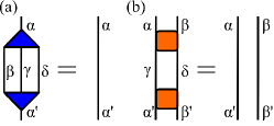
Figure 2: (Color online) Diagrammatic representation of the constraints for the isometries $w$ and disentanglers $u$ of the ternary MERA.

For an infinite lattice $\mathcal{L}_{0}$ one can perform infinite many RG transformations, resulting in a MERA tensor network similar to Fig. 1 with infinite sites and layers. Assuming translational invariance, a single pair of $(u_{\tau},w_{\tau})$ is enough to uniquely define the coarse-graining process into $\mathcal{L}_{\tau}$. For critical systems, after a finite number of RG transformations, the system becomes scale invariant at $\mathcal{L}_{s}$. After the system reaches scale invariance, further RG transformation will generate the same effective Hamiltonian and the lattice. Hence it suffices to use a single pair of $(u_{s},w_{s})$ to represent the RG transformations for $\mathcal{L}_{\tau}$ for $\tau\geq s$. Such a MERA structure is called scale invariant MERA in the literature.Pfeifer et al. (2009) In principle, the number of RG steps to reach scale invariance is a priori unknown and depends on the original Hamiltonian. In practice to keep the computation trackable one sets $s$ to some pre-determined number and layers $\mathcal{L}_{\tau},\tau=1,\cdots,s-1$ are called buffer layers in MERA terminology.

An advantage of the scale invariant MERA is its ability to directly extract scaling properties of a critical system. For example, scaling dimensions of primary fields and the central charge of the corresponding CFT can be obtained directly. Pfeifer et al. (2009) At scale invariant layers the RG transformation of operators is dictated by the scaling superoperator $\widetilde{S}$ which is a fixed-point RG map. The scaling operator $\phi_{i}$ with scaling dimension $\Delta_{i}$ should satisfy the equation

$$\widetilde{S}(\phi_{i})=\lambda_{i}\phi_{i}\;,\;\;\Delta_{i}\equiv-\log_{3}\lambda_{i}\;,$$ (4)

where the logarithmic base three reflects the three-to-one coarse-graining of the ternary MERA scheme. All scaling dimensions can be, in principle, obtained by evaluating eigenvalues of the superoperator.

As an example, we show the results of scaling dimensions for the 1D transverse Ising model at criticality. We set $s=5$ as the scale invariant layer, making $\tau=1,\cdots,4$ be the buffer layers. We first optimize $(u_{\tau},w_{\tau})$ and $(u_{s},w_{s})$ by the standard MERA algorithm. The superoperator $\widetilde{S}$ is then constructed from $(u_{s},w_{s})$ and diagonalized to obtain the (lowest few) scaling dimensions. One can also construct superoperator $\widetilde{S}_{\tau}$ from $(u_{\tau},w_{\tau})$, although the system is not yet scale invariant. In the same token, pseudo-scaling-dimensions $\Delta_{i}(\tau)$ for the buffer layers can be obtained by diagonalizing $\widetilde{S}_{\tau}$. These $\Delta_{i}(\tau)$’s are used to monitor how the system approaches the scaling invariance. Thereby, we calculate $\Delta_{i}(\tau)$ for each buffer layer to form a flow of the pseudo-scaling-dimension as illustrated in Fig. 3(a). We observe that the pseudo-scaling-dimension $\Delta_{1}(\tau)$ of buffer layers gradually approaches the value of the scaling dimension $\Delta_{1}$ of the scale invariant layers for $\tau\geq 5$. The exact value of $\Delta_{1}=1/8$ is also plotted as a reference. The above example shows that the scale invariant MERA provides a well-defined method to study the scaling properties of the RG fixed points. In the following, we will use this scheme to study the scaling properties of the junction of two interacting quantum wires.

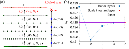
Figure 3: (Color online) (a) Four pairs of $(w_{\tau},u_{\tau})$ in buffer layers $(\tau=1,2,3,4)$ and the same copies of the scale invariant pair $(w_{s},u_{s})$ in the scale invariant layers are employed. Along the RG transformation axis, the pseudo-scaling-dimension $\Delta_{\sigma}(\tau)$ of buffer layers flows into the real scaling dimension $\Delta_{\sigma}$ of the scale invariant RG fixed point. (b) Both $\Delta_{\sigma}(\tau)$ and the scaling dimension of the spin primary field in the CFT are calculated, and the pseudo-scaling-dimension approaches the exact value as the layer $\tau$ is close to the scale invariant layers. The exact value of the scaling dimension of the spin primary field from the CFT is $1/8$ for the transverse Ising model. Cardy (2010) The bound dimension used here is $\chi=8$.

III Junction of two interacting quantum wires

We start by modeling the impurity as a junction linking two identical semi-infinite 1D wires with a total Hamiltonian $H=H_{w}+h_{B}$. Here, $H_{w}$ represents the lattice Hamiltonian of the wires at half-filling,

$$H_{\rm w}=\sum_{\mu\in I,II}\sum_{i=0}^{\infty}\left(-c^{\mu{\dagger}}_{i+1}c^{\mu}_{i}+h.c.+V\bar{n}^{\mu}_{i}\bar{n}^{\mu}_{i+1}\right),$$ (5)

while the hopping Hamiltonian at the junction is given by

$$h_{\rm B}=-t\left(c^{I{\dagger}}_{0}c^{II}_{0}+h.c.\right).$$ (6)

We denote $c^{\mu}_{i}$ ($c^{\mu{\dagger}}_{i}$) with $\mu\in I,II$ as the annihilation (creation) operator at the site $i$ of the wire $\mu$, $\bar{n}^{\mu}_{i}\equiv c^{\mu\dagger}_{i}c^{\mu}_{i}-1/2$, and $V$ as the nearest-neighbor interaction strength. Following the bosonzination scheme, Oshikawa et al. (2006) the wires can be represented in terms of continuum bosonic fields $\varphi^{\mu}$ and their dual fields $\theta^{\mu}$ by

$$H_{\rm w}(\varphi^{\mu},\theta^{\mu})=\sum_{\mu\in I,II}\frac{v}{4\pi}\int dx\left[g(\partial_{x}\varphi^{\mu})^{2}+\frac{1}{g}(\partial_{x}\theta^{\mu})^{2}\right],$$ (7)

where, in the range $|V|\leq 2$, the plasmon velocity $v$ and the Luttinger parameter $g$ are identified via the Bethe Ansatz at half filling as

$$v=\pi\frac{\sqrt{1-(V/2)^{2}}}{\arccos(V/2)},\quad g=\frac{\pi}{2\arccos(-V/2)}.$$ (8)

Hence, we have $g=1$ for noninteracting wires and $g<1$ ($g>1$) for repulsive (attractive) interactions.

In comparison with an infinite LL wire, the presence of the junction could change the scaling behavior of the correlation functions across the junction. Starting from the lattice operators, define the current operator $J^{\mu}_{j+\frac{1}{2}}$ and the fermion density operators $N^{\mu}_{j+\frac{1}{2}}$ on the bond between sites $j$ and $j+1$ as

$$J^{\mu}_{j+\frac{1}{2}}= i\left(c^{\mu{\dagger}}_{j+1}c^{\mu}_{j}-c^{\mu{\dagger}}_{j}c^{\mu}_{j+1}\right),$$ (9)

$$N^{\mu}_{j+\frac{1}{2}}= \frac{1}{2}\left(n^{\mu}_{j}+n^{\mu}_{j+1}-\langle n^{\mu}_{j}\rangle-\langle n^{\mu}_{j+1}\rangle\right).$$

With these lattice operators, two-point correlation functions, such as $\langle J^{I}(x)J^{II}(x)\rangle$ and $\langle N^{I}(x)N^{II}(x)\rangle$, can be evaluated using the boundary MERA. The evaluated correlation functions should exhibit power law decay as expected in a 1D scale invariant quantum critical system. To see how the CIBC emerges due to the presence of the impurity at the RG fixed point, it is useful to introduce incoming and outgoing chiral density operators $\rho^{\mu}_{in/out}(x)$, defined with respect to the junction, with the relations $J^{\mu}(x)=v(\rho^{\mu}_{out}(x)-\rho^{\mu}_{in}(x))$ and $N^{\mu}(x)=\rho^{\mu}_{out}(x)+\rho^{\mu}_{in}(x)$. It is worth to emphasize that these chiral densities are those diagonalizing the interacting Hamiltonian in Eq. (7) but not the chiral currents defined in the non-interacting bands.

Since the boundary condition will dictate both the long distance scaling behaviors and the amplitude of correlation functions of primary fields, Cardy and Lewellen (1991) the chiral density correlation functions change accordingly with respect to different CIBC. Rahmani et al. (2010) We can now decompose the two-points correlation functions with operators defined in Eq. (9) to obtain the chiral density correlation functions. For instance, we have, in the case of $\mu\neq\mu^{\prime}$,

$$\langle\rho^{\mu}_{out}(x)\rho^{\mu^{\prime}}_{in}(x)\rangle=-\frac{1}{2}\left(\frac{1}{v^{2}}\langle J^{\mu}(x)J^{\mu^{\prime}}(x)\rangle+\frac{1}{v}\langle N^{\mu}(x)J^{\mu^{\prime}}(x)\rangle\right),$$ (10)

where we have used $\langle\rho^{\mu}_{out(in)}\rho^{\mu^{\prime}\neq\mu}_{out(in)}\rangle=0$. In the presence of time reversal symmetry (which is our case), the second term in Eq. (10) always vanishes. Thereby, the chiral correlation functions between different wires are directly proportional to the current-current correlation function.

Since the bulk of the LL quantum wires remains conformal invariant in the presence of impurity, correlation functions, in general, follow power law behaviors. Therefore, we expect that the equal time current-current correlation function decays at long distance in the form

$$\left|\left\langle J^{\mu}(x)J^{\mu^{\prime}}(x)\right\rangle\right| \sim Ax^{-\alpha}\;,$$ (11)

for $\mu\neq\mu^{\prime}$. From RG prospect, the tunneling term between two LL wires is a relevant perturbation for attractive interactions, $g>1$, and is irrelevant for repulsive interaction, $g<1$. As a result, two semi-infinite LL wires effectively fuse into a single infinite LL wire at RG fixed point for $g>1$. Kane and Fisher (1992a) In this case, the leading contribution to the correlation function in Eq. (11) is universal regardless of the impurity strength, and has the prefactor $A=gv^{2}/8\pi^{2}$ and the exponent $\alpha=2$, c.f. Appendix C. Rahmani et al. (2010, 2012) Thus, for $g>1$ the stable RG fixed point is a perfect transmission RG fixed point.

On the other hand, another RG fixed point corresponds to two disconnected wires with a strict zero linear conductance for $g<1$. An immediate consequence of this fixed point is the vanishing of $1/x^{2}$ term for the current-current correlation function in Eq. (11). However, subleading contribution can come from the irrelevant boundary operators, which gives a faster power law decay with the exponent $\alpha>2$ and the prefactor depending on the strength of the impurity. Here, the exponent is non-universal and can be contingent on the detail of the impurity.

In the linear response regime, the chiral correlation functions in Eq. (10) can be used to determine the conductance across the impurity. From the conventional Kubo formula, Oshikawa et al. (2006)

$$G_{\mu\nu}=\lim_{{\omega}\rightarrow 0_{+}}-\frac{e^{2}}{\hbar}\frac{1}{{\omega}L}\int_{-\infty}^{\infty}d\tau\;e^{i{\omega}\tau}\\ \times\int_{0}^{L}dx\;\langle{\cal T}_{\tau}J^{\mu}(y,\tau)J^{\nu}(x,0)\rangle,$$ (12)

the imaginary-time ordered (indicated by ${\cal T}_{\tau}$) dynamical current-current correlation function for currents $J^{\mu}$ and $J^{\nu}$ on wires $\mu$ and $\nu$ is needed to evaluate the conductance. As the current operators can be represented in terms of the chiral density operators, we can decompose the non-chiral correlation function by chiral current correlation functions. For $\mu\neq\nu$, we have

$$\langle{\cal T}_{\tau}J^{\mu}(y,\tau)J^{\nu}(x,0)\rangle=\\ -v^{2}\left(\langle\rho^{\mu}_{out}(y,\tau)\rho^{\nu}_{in}(x,0)\rangle+\langle\rho^{\mu}_{in}(y,\tau)\rho^{\nu}_{out}(x,0)\rangle\right),$$ (13)

where we have used the fact that correlation functions vanish for the same chiral current in different wires. In the presence of the conformal symmetry and the CIBC, one can show that the chiral correlation functions in Eq. (13) is always a function of $z=v\tau\mp\mathrm{i}(x+y)$. Rahmani et al. (2010) As a result, the dynamical chiral current correlation functions can be reconstructed via the static correlation functions shown in Eq. (10). Finally, the fixed-point conductance can be subsequently evaluated using the Kubo formula in Eq. (12).

IV Boundary MERA

The boundary CFT predicts that each boundary RG fixed point is associated with a CIBC and hence a conformally invariant boundary state. Cardy (2010) As a result, scaling behavior of the boundary operators are directly controlled by the realized boundary condition. In addition, even though the scaling dimensions of bulk primary operators, such as the chiral current operators, remain unchanged in the presence of a boundary, the coefficients of their correlation functions are dictated by the given boundary state. Thereby, constructing the corresponding boundary state allows us to obtain the full properties of a junction at its RG fixed point. Cardy and Lewellen (1991) In this section, we will discuss how to obtain the boundary state using a numerical boundary MERA scheme. For a complete review of the MERA algorithm and detailed discussion on the MERA with impurities, we refer the interested readers to Refs. Vidal, 2007; Evenbly and Vidal, 2013b, a.

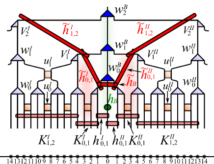
Figure 4: (Color online) Sketch of the boundary scale invariant MERA structure for three layers. The central tensors $w_{\tau}^{B}$ are used to represent the boundary state inside the causal cone (light green shaded area) of the green impurity. $\widetilde{h}^{\mu}_{\tau,\tau+1}$ is an effective two-site boundary Hamiltonian which is obtained by inhomogeneous coarse-graining, related to the causal cone of $K^{\mu}_{\tau,\tau+1}$ such as the red shaded area. Here $w^{\mu}_{\tau}$, $u^{\mu}_{\tau}$, and $V^{\mu}_{\tau}$ are bulk isometries , bulk disentanglers, and boundary truncation tensors respectively. The effective impurity Hamiltonian $\widetilde{h}_{B}$ is constructed from the impurity Hamiltonian $h_{B}$ and two-site Hamiltonian $h^{I}_{0,1}$ and $h^{II}_{0,1}$ in the bulk wires. Two quantum wires are connected in the junction, and we also label the site indices for each wire.

In Fig. 4 we sketch the MERA structure that describes two semi-infinite wires with a junction. First, two sets of standard bulk scale invariant MERA with isometries $w^{\mu}_{\tau}$ and disentanglers $u^{\mu}_{\tau}$ of bond dimension $\chi$ are used to describe the two semi-infinite wires. Second, the bare Hamiltonian at the original lattice are regrouped into $K^{\mu}_{\tau,\tau+1}$ and inhomogeneously ascended using the truncation tensors $V^{\mu}_{\tau}$ with bond dimension $\chi^{B}$, $w^{\mu}_{\tau}$, and $u^{\mu}_{\tau}$ to form the boundary Hamiltonian $\widetilde{H}_{B}$ . Finally the central tensor $w^{B}_{\tau}$ is used to describe the boundary state and is optimized via the boundary Hamiltonian $\widetilde{H}_{B}$. In a nutshell, the scale invariant boundary state is represented by the scale invariant central tensor $w^{B}_{\tau}$ in the boundary MERA. In the following we summarize the major steps of the boundary MERA algorithm, and we refer the readers to the Appendix for more details:

Optimization of the bulk scale invariant MERA – MERA is a specific scheme to perform real-space RG transformations using isometries $w^{\mu}_{\tau}$ (light blue triangles) and disentanglers $u^{\mu}_{\tau}$ (yellow squares) as shown in Fig. 4. Evenbly and Vidal (2009) In each RG step, to construct the coarse-grained Hamiltonian at the next layer $\tau+1$, the disentangler $u^{\mu}_{\tau}$ is used to transform to a less entangled local basis between blocks while the isometry $w^{\mu}_{\tau}$ is used to perform coarse-graining. They are optimized using the bulk scale invariant MERA algorithm. Avella and Mancini (2013) The algorithm minimizes the energy per site associated with the bare Hamiltonian, shown as the light pink bars at the bottom of Fig. 4. In this step, each wire is treated as independent and the associated $u^{\mu}_{\tau}$ and $w^{\mu}_{\tau}$ are optimized independently. In this work, the two wires are identical, so the bulk optimization needs to be carried out only once.

Construction of the effective boundary Hamiltonian – A key step of the boundary MERA is to perform an inhomogeneous coarse-graining of the bare Hamiltonian to obtain an effective boundary Hamiltonian $\widetilde{H}_{B}$. Evenbly et al. (2010) The boundary Hamiltonian for the chain of the central tensors $w^{B}_{\tau}$ consists of the effective impurity Hamiltonian $\widetilde{h}_{B}$, pictorially defined in Fig. 5 (a) and two-site Hamiltonians $\widetilde{h}^{\mu}_{\tau,\tau+1}$ that connect two adjacent sites $\tau$ and $\tau+1$ as depicted as red bars in Fig. 4:

$$\widetilde{H}_{B} =\widetilde{h}_{B}+\sum_{\mu\in I,II}\sum_{\tau=0}^{\infty}\widetilde{h}^{\mu}_{\tau,\tau+1}.$$ (14)

Here, $\widetilde{h}^{\mu}_{\tau,\tau+1}$ is constructed from the inhomogeneous ascending of a collection $K^{\mu}_{\tau,\tau+1}$ of bare Hamiltonians $h_{i,i+1}^{\mu}$ at the same scale

$$K^{\mu}_{\tau,\tau+1} =\sum_{i=s(\tau)}^{s(\tau+1)-1}h_{i,i+1}^{\mu}\;,$$ (15)

where $s(\tau)=(3^{\tau+1}-1)/2$ with $\tau=0,1,2,3,\cdots$, and $h_{i,i+1}^{\mu}$ is a two-site Hamiltonian in wire $\mu$. The boundary Hamiltonian $\widetilde{h}^{\mu}_{\tau,\tau+1}$ is obtained by inhomogeneous coarse-graining two-site bulk Hamiltonian in layer $\tau$ via the inhomogeneous ascending superoperator $\overline{A}_{\rm bd}^{\mu}[h_{1,2}^{\mu}(\tau),h_{2,3}^{\mu}(\tau),h_{3,4}^{\mu}(\tau)]$, with a scaling factor $1/3$ which reflects the ternary MERA. For instance, to obtain the boundary Hamiltonian $\widetilde{h}^{\mu}_{0,1}$, we construct $\overline{A}_{\rm bd}^{\mu}[h_{1,2}^{\mu}(\tau=0),h_{2,3}^{\mu}(\tau=0),h_{3,4}^{\mu}(\tau=0)]$ for $K_{0,1}^{\mu}$ in Fig. 5 (b)-(c) by contracting the tensors inside the causal cone (shaded red area in Fig. 4). Moreover, in order to assign a different bond dimension $\chi^{B}$ to the central tensor $w^{B}_{\tau}$, we introduce a truncation tensor $V^{\mu}_{\tau}$ at the boundary. We note that in general $\chi^{B}$ can be layer dependent until the central tensor $w^{B}_{\tau}$ reaches scale invariant, after which only one single $\chi^{B}$ is used for all the scale invariant layers.

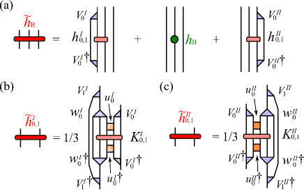
Figure 5: (Color online) (a) Graphic representation of $\widetilde{h}_{B}$ including the impurity Hamiltonian $h_{B}$ and the inhomogeneous coarse-graining of the first two-site Hamiltonian $h_{0,1}^{\mu}$ in wire $\mu\in I,II$. (b)-(c) Using inhomogeneous coarse-graining to obtain the boundary Hamiltonian $\widetilde{h}_{0,1}^{\mu}$ with a scaling factor $1/3$ for wire $I$ and $II$, respectively.

Optimization of the central tensors – The final step is to utilize the boundary Hamiltonian (red bars) to optimize the central tensors $w_{\tau}^{B}$ (blue triangles) which represent the boundary state in the boundary chain (shaded green). Here we employ a scale invariant boundary MERA algorithm to optimize the central tensors $w^{B}_{\tau}$. Similar to the bulk MERA, we treat the energy per site as the cost function for the optimization processes. The energy of the boundary MERA can be calculated at layer $\tau$ as

$$E ={\rm tr}\{w_{\tau}^{B}Y_{\tau}\}\;,$$ (16)

where $Y_{\tau}$ is the environment associated with $w_{\tau}^{B}$. In general, it is necessary to insert several buffer layers with different central tensors $w_{0}^{B},w_{1}^{B},\cdots,w_{\tau_{{\it bf}-1}}^{B}$ before one reaches the scale invariant layers characterized by a single central tensor $w_{s}^{B}$. For the buffer layers and the scale invariant layers the environment construction differs. The environment for the former can be obtained by the procedure defined in Appendix  B. The environment for the scale invariant layers is constructed from the scale invariant Hamiltonian

$$\widetilde{h}_{s}^{\mu}=\sum_{\tau=\tau^{\prime}_{s}}^{\infty}\frac{\widetilde{h}_{\tau,\tau+1}^{\mu}}{3^{\tau-\tau^{\prime}_{s}}}\;,$$ (17)

where the layer $\tau$ starts from the second scale invariant layer $\tau^{\prime}_{s}=\tau_{s}+1$, and all layers beyond layer $\tau_{s}$ are scale invariant. Here the factor three reflects the three-to-one coarse-graining. In practice, it is useful to introduce a cutoff to replace the infinite sum by a finite sum (see Appendix).

Given the effective Hamiltonian $\widetilde{H}_{B}$, we perform an optimization procedure based on the boundary MERA framework. Evenbly et al. (2010) The procedure is similar to optimizing the scale invariant MERA and allows us to construct an scale invariant boundary state. We describe the details of the construction of the boundary MERA tailored for the two-wire junction in the Appendix. In all calculations below we always set to have two buffer layers and enforce the system to have scale invariance starting from the third layer.

V Current-current correlation functions

As stated previously, the current-current correlation functions across the junction provide important information on the transport properties. To simplify the calculations, we perform a Jordan-Wigner transformation to map the spinless fermion model into a spin-1/2 XXZ model. We consider two semi-infinite wires, labeled by $\mu=I,II$, and the transformation is defined as

$$c^{\mu}_{j} =S^{\mu-}_{j}e^{{\rm i}\pi\Phi_{j}^{\mu}}\;,$$ (18)

$$c^{\mu\dagger}_{j} =S^{\mu+}_{j}e^{-{\rm i}\pi\Phi_{j}^{\mu}}\;.$$ (19)

The site index $j$ goes from zero to infinity in each wire, and the junction connecting the two wires is at site zero (see Fig. 4). In addition, the phase factor $\Phi_{j}^{\mu}$ is defined as

$$\Phi_{j}^{I} =\sum_{k=\infty}^{j+1}S^{I+}_{k}S^{I-}_{k}\;,$$ (20)

$$\Phi_{j}^{II} =\sum_{k=\infty}^{0}S^{I+}_{k}S^{I-}_{k}+\sum_{k=0}^{j-1}S^{II+}_{k}S^{II-}_{k}\;.$$ (21)

Additionally the current operator in Eq. (9) in the spin language is written as

$$J_{j+\frac{1}{2}}^{\mu}={\rm i}(S^{\mu-}_{j}S^{\mu+}_{j+1}-S^{\mu+}_{j}S^{\mu-}_{j+1})\;.$$ (22)

Once an optimal boundary MERA state is obtained, we can evaluate the current-current correlation function in the presence of the junction. For the lattice model, we calculate $\left|\left\langle J^{\mu}_{j+\frac{1}{2}}J^{\mu^{\prime}}_{j+\frac{1}{2}}\right\rangle\right|$, where $j+\frac{1}{2}$ denotes the current from the $j$-th to the $(j+1)$-th site. $x=(j+\frac{1}{2})$ defines the distance from the boundary.

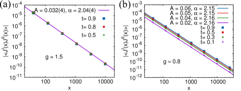
Figure 6: (Color online) The current-current correlation function as a function of the distance from the boundary. (a) Universal behavior with the same $A=0.032,\alpha\approx 2$ for $g=1.5$ with various $t=0.5,0.8,0.9$ is observed. (b) Non-universal behavior with distinct $A$ and $\alpha>2$ for $g\approx 0.8$ and $t=0.9,0.5,0.3,0.1$. The calculations are carried out using $\chi=12$ and $\chi^{B}=24$.

In the following we show our numerical results of current-current correlation function for $g=1.5$ and $g\approx 0.8$ as representatives for the $g>1$ and $g<1$ fixed points respectively. For $g>1$ the RG fixed point corresponds to a healed single wire. Furthermore, the boundary CFT predicts that the prefactor $A$ and the exponent $\alpha$ in Eq. 11 are universal regardless the strength of the junction. In Fig. 6(a) we show the current-current correlation function for the case of $g=1.5$ and $t=0.5,0.8,0.9$ for large distance. We observe that all data points fall on a universal line with the same exponent $\alpha=2.04(4)$ and the same prefactor $A=0.032$. These results agree well with the boundary CFT’s prediction of $A=gv^{2}/8\pi^{2}$ using the velocity $v\approx 1.299$ from Eq. (8). For very short distance, we find that the current-current correlation functions depend on the coupling strength of the weak link. We employ two buffer layers before we enforce scale invariance in our current MERA scheme; therefore, for distance longer than a characteristic length scale $x_{s}=\frac{3^{3}-1}{2}=13$, the correlation function is dictated by the RG fixed point and shows a universal behavior. For distance $x<x_{s}$, however, the the correlation function depends on the strength of the weak link.

In contrast, for $g<1$, the RG fixed point corresponds to two disconnected wires and the universal behavior is not expected. Consequently, to the leading order, the coefficient in front of the correlation functions is zero and the sub-leading corrections from the irrelevant operators at the boundary will be observed. Since the scale invariance of the MERA scheme is enforced, the correlation function will still show a power-law decay but with an exponent that is larger than 2 with a non-universal prefactor. In Fig. 6(b) we show the results for the case of $g\approx 0.8<1$ and $t=0.1,0.3,0.5,0.9$. Indeed we observe that different $t$ results in different scaling behavior with the exponents $\alpha>2$. Similarly for short distance $x<13$ we also observe non-universal behavior since the system is not yet dictated by the RG fixed point. The distinct behavior of the correlation function for $g>1$ and $g<1$ indicates that the system flows into different RG fixed points. Even without the a priori knowledge about the analytical results for the number and the nature of the RG fixed points, the numerical results can distinguish the two RG fixed points.

Furthermore, the conductance for the two-wire model can be estimated by the Kubo formula using the current-current correlation function.Kane and Fisher (1992b); Rahmani et al. (2010) For $g>1$, we expect that the system is dictated by a total transmission fixed point, i.e., two wires are fused into a single LL wire. The exponent in the current-current correlation function is hence $\alpha=2$, leading to the conductance

$$G_{I,II}=g\frac{e^{2}}{h}.$$

On the other hand, for $g<1$, we expect the two wires are effectively disconnected, which corresponds to a total reflection fixed point. In this case, the current-current correlation function between two wires should decay faster than $1/x^{2}$, resulting in a zero conductance. Our results discussed above hence shows that one can use boundary MERA to classify fixed points from the exponent of the current-current correlation function. In the following section, we will show a more direct way to identify the fixed points using the scaling dimensions of the boundary operators.

VI Spin-spin correlation functions and scaling dimensions

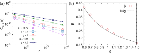
Figure 7: (Color online) (a) The spin-spin correlation function in Eq. (23) as a function of the distance between two spin operators for a bulk wire with $g\approx 0.79,0.9,1,1.24,1.5$. (b) The exponent $\beta$ of the spin-spin correlation function as a function of $g$. The calculations are carried out using $\chi=16$.

We next study the two-point spin-spin correlation function defined as

$$C_{S^{+}S^{-}}(r) =\left|\langle S^{+}(r_{1})S^{-}(r_{2})\rangle-\langle S^{+}\rangle\langle S^{-}\rangle\right|\;,$$ (23)

where $r_{1}$=$r_{2}$ is the distance from the spin operator to the impurity site on the wire $I$ and $II$ respectively. $r=|r_{1}|+|r_{2}|$ is the distance between two spin operators of $S^{+}(r_{1})$ and $S^{-}(r_{2})$. The correlation function shows a power-law decay,

$$C_{S^{+}S^{-}}(r)=\alpha r^{-2\beta}\;,$$ (24)

where $\beta$ should be equal to the second lowest scaling dimension $\Delta_{2}$ of the bulk LL wire. The lowest scaling dimension $\Delta_{1}=0$ which corresponds to the scaling operator of the identity, and is independent of the Luttinger parameter $g$. The lowest non-vanishing scaling dimension $\Delta_{2}$, however, varies with $g$ as $1/4g$. In the spin language of the $XXZ$ model, this is the scaling dimension of the primary fields $S^{\pm}$, leading to a power-law decay of the spin-spin correlation function. In Fig. 7(a), we plot the spin-spin correlation functions for several $g$ in the bulk wire. We clearly observe that for all $g$’s, the spin-spin correlation functions show a power-law decay. In Fig. 7(b) we show the fitted exponent $\beta$ as a function of $g$. The results agree well with the expected value of $\beta=\Delta_{2}=1/4g$. Since the exponents are dictated by the scaling dimensions of the primary fields, this provides an indirect way to study the scaling dimensions. We will demonstrate how to study scaling dimensions directly in the MERA later in this subsection.

To study the effects of the boundary we investigate how the behavior of spin-spin correlation function depends on the strength $t$ of the impurity. In Fig. 8(a) and (b) we show the results for $g=1.5$ and $g\approx 0.8$ respectively with $t=0.1,0.5$, and $0.9$. For $g>1$, we again observe a universal behavior that all correlation functions fall on the same line regardless the strength $t$ of the impurity. Furthermore, the line is actually the same as the one for the bulk wire. In contrast for $g<1$, non-universal behavior is observed. The pre-factor $a$ depends strongly on the value of $t$. The exponent $\beta$, however, remains the same as the bulk value. We comment that even without the a priori knowledge on the exact nature of the fixed points, the results obtained by MERA clearly indicate that there are two distinct fixed points corresponding to the case of $g>1$ and $g<1$ respectively. For problems with unknown RG fixed points, in principle it is possible to identify the RG fixed points by studying the behavior of different two-point correlation functions.

Another way to directly identify unknown RG fixed points is to study the scaling dimensions of the boundary scaling operators which can be straightforwardly obtained by boundary MERA. Identifying operator contents of primary fields and their descendants are the most essential step to quantify the properties of a conformally invariant system. These scaling operators $\phi_{\alpha}^{B}$ follow specific rule under the scaling transformation and have the scaling dimensions $\Delta_{\alpha}^{B}$. Similar to the scale invariant bulk MERA Pfeifer et al. (2009), in the scale invariant layer the boundary scaling superoperator $\widetilde{\mathcal{S}}^{B}$ which can be expressed in terms of central tensor $w^{B}_{s}$ as

$$\left[\widetilde{\mathcal{S}}^{B}\right]^{\alpha,\delta^{\prime}}_{\delta,\alpha^{\prime}}= \sum_{\beta,\gamma}\left[w^{B}_{s}\right]^{\alpha}_{\beta,\delta,\gamma}\left[{w_{s}^{B}}^{\dagger}\right]_{\alpha^{\prime}}^{\beta,\delta^{\prime},\gamma}\;.$$

Here, the upper index ^B indicate that superoperator is evaluated at the boundary. Then, one can show that the boundary scaling operators $\phi_{\alpha}^{B}$ are the eigen-operators of superoperator $\widetilde{\mathcal{S}}^{B}$ and have the relations Pfeifer et al. (2009); Evenbly and Vidal (2009); Evenbly et al. (2010)

$$\widetilde{\mathcal{S}}^{B}(\phi_{\alpha}^{B})=\lambda_{\alpha}^{B}\phi_{\alpha}^{B},~{}~{}~{}~{}~{}\Delta_{\alpha}^{B}\equiv-\log_{3}\lambda_{\alpha}^{B}.$$ (25)

The base three of the logarithm reflects the mapping of three sites into one during the coarse-graining. Now, the scaling dimensions $\Delta_{\alpha}^{B}$ of scaling operators are obtained simply by the eigenvalue decomposition of the $\widetilde{\mathcal{S}}^{B}$. Numerically, with the finite boundary bond dimension $\chi^{B}$, the maximum number of scaling dimensions, which we can evaluate from boundary MERA, is constrained to be $(\chi^{B})^{2}$.

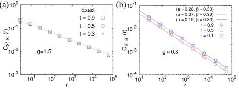
Figure 8: (Color online) The spin-spin correlation function in Eq. (23) as a function of the distance between two spin operators crossing the junction for various $g$, and we chose two spin operators have same distance far away from the boundary. (a) The universal behavior at the perfect transmission fixed point for $g=1.5$ with $t=0.3,0.5,0.9$, the exact solution Lukyanov (1998); Lukyanov and Terras (2003) describes the character of the bulk. (b) The non-universal behavior at the total reflection fixed point for $g\approx 0.8$ with $t=0.1,0.5,0.9$, and the lines are the fitting results of $C_{S^{+}S^{-}}(r)\approx ar^{-2\beta}$.

The boundary scaling dimensions are expected to show different dependence on the Luttinger parameter $g$, but are independent from the hopping amplitude $t$ at the the junction. First, we expect that $\Delta^{B}_{2}(g>1)=1/4g$ has the same Luttinger liquid parameter dependence as that in the bulk. This is due to the fact that the boundary RG fixed point at $g>1$ corresponds to the perfect transmission between two wires and two semi-infinite LL wires effectively heal to one infinite LL wire. On the other hand, the RG fixed point for $g<1$ corresponds to a total reflection boundary condition for both wires. Due to the current conservation, the incoming current is perfectly reflected to the outgoing current at the boundary for both wires. Therefore the current operators are pinned at boundary, i.e., $\theta^{I,II}|_{x=0}=0\to\phi_{in}|_{x=0}=\phi_{out}|_{x=0}$, which lead to the change of scaling dimensions of boundary operators. (c.f. Ref. Oshikawa et al., 2006 for detailed arguments.) The spin operators at boundary now become $S^{\pm}\sim e^{\pm i\sqrt{g/2}\varphi}\to S^{\pm}|_{x=0}e^{\pm\sqrt{2g}\phi_{in}}$, Oshikawa et al. (2006); Lukyanov (1998) and have scaling dimension $\Delta^{B}_{2}=1/2g$.

The lowest non-vanishing bulk and boundary scaling dimensions are evaluated and shown as red triangles and blue squares in Fig. 9, respectively. First and foremost, the bulk scaling dimension fits very well with the expected functional dependence $\Delta_{2}=1/4g$ while the boundary scaling dimension $\Delta_{2}^{B}(g)$ exhibits a drastic change at $g=1$. Numerically, we found $\Delta^{B}_{2}(g>1)=1/4g$, the same Luttinger liquid parameter dependence as in the bulk. For $g<1$, we observed that the functional dependence of $\Delta^{B}_{2}(g<1)$ fits very well with $1/2g$. These results are consistent with fact that two different boundary RG fixed points are realized at $g>1$ and $g<1$.

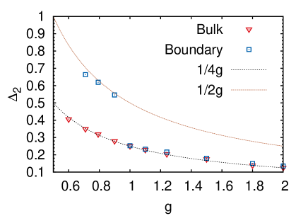
Figure 9: (Color online) The lowest few non-vanishing scaling dimensions of primary fields of the bulk and boundary as a function of Luttinger parameters $g$. The calculations are carried out using $\chi=12$ and $\chi^{B}=24$.

VII Conclusions

We have used the boundary MERA framework to classify two fixed points in a simple two-wire case shown by Kane and Fisher. By keeping explicitly the scale invariance of the boundary state we can obtain current-current correlation functions that decay as a power law with either a universal or non-universal exponent and prefactor, depending on the RG fixed point reached. We can also obtain the bulk and boundary scaling dimensions that agree perfectly with the formal RG analysis. This establishes firmly the boundary MERA as a numerical method to determine the RG fixed point and the universal conductance of quantum two-wire junctions.

The method has the advantage that it can be easily extended to study multi-wire junctions. Even in the simplest case, the Y-junction with three LL wires, not all the fixed points are fully understood by the CFT. Oshikawa et al. (2006) We expect that boundary MERA can provide a new approach to gain insights into the properties of possible RG fixed points and their classification for more complicated multi-wire junctions, Lal et al. (2002); Chen et al. (2002); Egger et al. (2003); Pham et al. (2003); Kazymyrenko and Doucot (2005); Das and Rao (2008); Bellazzini et al. (2009); Aristov et al. (2010); Aristov (2011); Aristov and Wölfle (2011) spinful LL wires,Hou and Chamon (2008) junctions of LL wires with different interaction strength in each wireSafi and Schulz (1995); Maslov and Stone (1995); Aristov and Wölfle (2012); Hou et al. (2012); Aristov and Wölfle (2013), and junctions of Josephson-Junction networks.Cirillo et al. (2011); Giuliano and Sodano (2013) Potentially, the boundary MERA also provides an unbiased numerical RG method to resolve the issue about whether the conductance of Y-junction can break the single particle unitarity in the strong attractive interaction regime. Oshikawa et al. (2006); Aristov and Wölfle (2011)

In addition, since we optimize the bulk scale invariant MERA independently of the boundary, the bulk results can be reused. This potentially can significantly reduce the computational costs, and can have the advantage over the DMRG method proposed in Ref. Rahmani et al., 2010. Moreover, the scaling dimensions of the primary fields at the impurity site can be directly obtained, which can provide crucial information about the associated boundary CFT and enable further classifications of the RG fixed points. Wong and Affleck (1994); Oshikawa et al. (2006); Hou and Chamon (2008) While the conductance of multi-wire junctions has been calculated by CFT, however, only very few numerical calculations exist in the literature to quantitatively study and classify these results in details. In the MERA framework, none of the theoretical manipulation required in the DMRG is necessary, and a direct computation of the current-current correlation function is possible. This provides a systematic and direct numerical method to study the effects of strong electron-electron interactions in the transport properties of quantum impurity problems and molecular electronic devices.

Appendix A Scale invariant boundary MERA

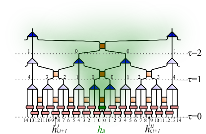
Figure 10: (Color online) Ternary MERA for three layers with an impurity at the junction described by $h_{B}$. The shaded green is the causal cone for the junction. The two-site Hamiltonian $h_{i,i+1}^{\mu}$ for layer $\tau=0$ (pink bars) is described in Eq. (28). We also label site indices in each layer running from zero to infinity for both wires. The light blue triangles and the light yellow squares represent bulk isometries and bulk disentanglers, respectively.

The boundary MERA framework used in this work is based on a ternary bulk MERA of two semi-infinite wires with a junction as shown in Fig. 10. The shaded green area represents the casual cone associated with the junction that is described by $h_{B}$. It is clear from the figure that when one connects two wires with a junction, one does not need to re-optimize the MERA structure associated with the bulk part of the wires (light color tensors). The tensors in the shaded green area, however, need to be re-optimized. To simplify the structure of the boundary MERA, we fuse tensors inside the green shaded area to form a rank-four central tensors $w_{\tau}^{B}$ with four external legs at each layer (Fig. 4). Within the boundary MERA framework, the boundary state is characterized by these central tensors.

We introduce both the boundary truncation tensors $V^{\mu}_{\tau}$ and the boundary tensors $B^{\mu}_{\tau}$ to reduce the computational cost and the memory storage during the optimization of the central tensors. The boundary truncation tensors $V^{\mu}_{\tau}$ allow the bond dimensions of the central tensors to be different from the bond dimensions of the bulk MERA tensors. For simplicity, all tensors here are scale invariant, and each bond of bulk $w^{\mu}_{\tau}$ has the same bond dimension $\chi$. As shown in Fig. 11(a), both $V^{\mu}_{\tau}$ and $B^{\mu}_{\tau}$ are obtained by decomposing the rank-four bulk isometry $w^{\mu}_{\tau}$ as two rank-three tensors that satisfies the equation

$${\rm tr}\{w^{\mu\,\dagger}_{\tau}V_{\tau}^{\mu}B_{\tau}^{\mu}\rho^{\mu}_{\tau+1}\} =1\;,$$ (26)

where $\rho^{\mu}_{\tau+1}$ is bulk one-site density matrix. When truncation is necessary, one can truncate the bond linking the $V^{\mu}_{\tau}$ and $B^{\mu}_{\tau}$ to some number $\chi^{B}\leq\chi^{2}$. We note that $V_{\tau}^{\mu}$ of all possible layers satisfies the orthogonal condition $V^{\mu\dagger}_{\tau}\,V^{\mu}_{\tau}=\mathbf{1}$ as shown in Fig. 11(b). Conceptually, we fuse $B^{I}_{\tau}$, $B^{II}_{\tau}$ and the boundary disentangler $u^{B}_{\tau}$ in the green causal cone of Fig. 10 to form the rank-four central tensor $w^{B}_{\tau}$ in Fig. 4 by the contraction shown in Fig. 11(c). With all the derivation above, one arrives at the MERA structure describing two-wires with a junction, as shown in Fig. 4. We refer to Ref. Evenbly and Vidal, 2013a for optimization details of both boundary truncation tensors and boundary tensors.

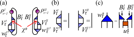
Figure 11: (Color online) (a) Graphic representation of Eq. (26). An isometry is decomposed into two tensors $V_{\tau}^{\mu}$ and $B_{\tau}^{\mu}$ linked in the truncated bond dimension $\chi^{B}$. (b) The isometric conditions of $V_{\tau}^{\mu}$ for $\mu\in\;I,II$. The lines at the right hand side of equal signs are identity matrices. (c) Construct a central tensor $w_{\tau}^{B}$ from three tensors $B^{I}_{\tau}$, $B^{II}_{\tau}$, and $u_{\tau}^{B}$.

A.1 Boundary Hamiltonian $\widetilde{H}_{B}$

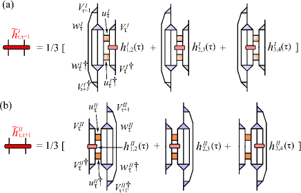
Figure 12: (Color online) Graphic representation of $\widetilde{h}_{\tau,\tau+1}^{\mu}$ (a) for wire $I$ and (b) for wire $II$.

In this section we describe how to construct the effective boundary Hamiltonian from the bare Hamiltonian of a general two-wire model:

$$H =h_{B}+H_{\rm w}\;,$$ (27)

$$H_{\rm w} =\sum_{\mu\in I,II}\sum_{i=0}^{\infty}h^{\mu}_{i,i+1}\;,$$ (28)

where $h_{B}$ is the on-site impurity Hamiltonian shown as the green circle in Fig. 4, and $H_{\rm w}$ represents two semi-infinite Hamiltonian for wires $\mu\in I,II$. We assume that the wire Hamiltonian can be expressed as a sum of nearest-neighbor interactions in Eq. (28). In particular, for the spin-1/2 XXZ model considered in this work, one has

$$h_{B} =-t(S^{I\,+}_{0}S^{II\,-}_{0}+S^{I\,-}_{0}S^{II\,+}_{0})\;,$$ (29)

$$h^{I}_{i,i+1} =J(S^{I\,X}_{i+1}S^{I\,X}_{i}+S^{I\,Y}_{i+1}S^{I\,Y}_{i})+\lambda S^{I\,Z}_{i+1}S^{I\,Z}_{i}\;,$$ (30)

$$h^{II}_{i,i+1} =J(S^{II\,X}_{i}S^{II\,X}_{i+1}+S^{II\,Y}_{i}S^{II\,Y}_{i+1})+\lambda S^{II\,Z}_{i}S^{II\,Z}_{i+1}\;.$$ (31)

There are two stages in constructing the effective boundary Hamiltonian:

Regrouping the bare Hamiltonian– As shown in Fig. 4, we regroup the bare Hamiltonian into $K^{\mu}_{\tau,\tau+1}$ according to Eq. (15), where $\tau$ is layer index. Apply a sequence of average bulk ascending processes on the subset Hamiltonian $K^{\mu}_{\tau,\tau+1}$ until layer $\tau$ is reached,

$$h^{\mu}_{i,i+1}(\tau) =\overline{A}_{\rm bulk}[h^{\mu}_{j,j+1}(\tau-1)]\;,$$ (32)

where $h^{\mu}_{i,i+1}(\tau)$ is the two-site bulk Hamiltonian in layer $\tau$, and $\overline{A}_{\rm bulk}$ is the bulk average ascending superoperator in the MERA framework. Evenbly and Vidal (2009) In addition, if we consider a translational invariant bulk MERA, within the same layer $\tau$, $h^{\mu}_{i,i+1}(\tau)$ remains the same for different sites due to the translational invariance.

Performing the inhomogeneous ascending operation– The two-site boundary Hamiltonian $\widetilde{h}_{\tau,\tau+1}^{\mu}$ is obtained by an inhomogeneous coarse-graining of bulk two-site Hamiltonians $h^{\mu}_{i,i+1}(\tau)$ in layer $\tau$. By applying bulk ascending process on $K_{\tau,\tau+1}^{\mu}$, we obtain $h^{\mu}_{i,i+1}(\tau)$, and we employ the inhomogeneous boundary coarse-graining with a scaling factor $1/3$ (Fig. 12),

$$\widetilde{h}_{\tau,\tau+1}^{\mu} =\overline{A}_{\rm bd}^{\mu}[h^{\mu}_{1,2}(\tau)+h^{\mu}_{2,3}(\tau)+h^{\mu}_{3,4}(\tau)]\;.$$ (33)

Once the boundary Hamiltonian is obtained, we can forget about the bulk tensors and concentrate on the optimization of the central tensors $w^{B}_{\tau}$ with the effective boundary Hamiltonian $\widetilde{H}$. Therefore, the tensor network in the boundary MERA is simplified (Fig. 13), and we perform optimization to obtain $w_{\tau}^{B}$. The central density matrix $\rho_{\tau}$ and the central Hamiltonian $\widetilde{h}^{\rm c}_{\tau}$ are fundamental building blocks during the updates, and they can be descended and ascended using descending and ascending superoperators described in the following section.

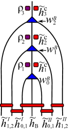
Figure 13: (Color online)The red bars represent the effective boundary Hamiltonian consisting of $\widetilde{h}_{\tau,\tau+1}$ and $\widetilde{h}_{B}$. $w_{\tau}^{B}$ are the central tensors indicated by blue triangles. $\rho_{\tau}$ and $\widetilde{h}^{\rm c}_{\tau}$ are central density matrices and central Hamiltonian, respectively.

A.2 Central ascending and descending processes

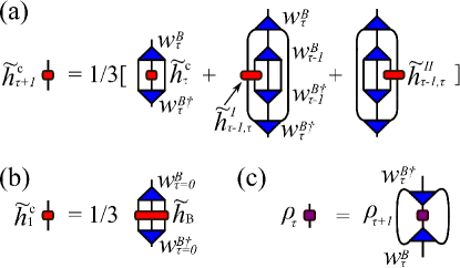
Figure 14: (Color online) (a) The average central ascending process for $\widetilde{h}^{\rm c}_{\tau+1}$. (b) $\widetilde{h}^{\rm c}_{1}$ is carried out using the ascending operation of the effective Hamiltonian $\widetilde{h}_{B}$, described in Fig. 5 (a). (c) The descending superoperator $D^{\rm c}$ composes of $w^{B}_{\tau}$ and $w_{\tau}^{B\dagger}$, and it acts on $\rho_{\tau+1}$ to obtain the central density matrix $\rho_{\tau}$.

Similar to the bulk MERA, an operator that lives on the effective boundary lattice can be RG-transformed to the next or previous layer via central ascending or descending superoperators. In this section we describe how to construct the central ascending and descending superoperators. Typically one use the ascending superoperator to ascend the Hamiltonian and use the descending superoperator to descend the density matrix.

First, the central Hamiltonian $\widetilde{h}^{\rm c}_{\tau+1}$ for $\tau\geq 1$ can be obtained from the lower layer using the central ascending superoperator (Fig. 14 (a) ),

$$\widetilde{h}^{\rm c}_{\tau+1} =\overline{A}(\widetilde{h}_{\tau}^{\rm c},\widetilde{h}_{\tau-1,\tau}^{I},\widetilde{h}_{\tau-1,\tau}^{II})\;.$$ (34)

The central ascending for $\tau=0$ is defined slightly differently (Fig. 14 (b)),

$$\widetilde{h}^{\rm c}_{1} =\overline{A}_{0}(\widetilde{h}_{\rm B})\;.$$ (35)

Second, we show how to perform central descending superoperator on the central density matrix. In contrast to the ascending superoperators, there is only one tensor network associated with the central descending superoperator ${D}^{c}$ consisting of both $w^{B}_{\tau}$ and $w^{B\dagger}_{\tau}$ as shown in Fig. 14 (c). The central density matrix at layer $\tau$ is then obtained by applying the central descending superoperator $D^{\rm c}$ to the central density matrix at layer $\tau+1$ as

$$\rho_{\tau} =D^{\rm c}(\rho_{\tau+1}).$$ (36)

Appendix B Optimization of central tensors

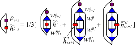
Figure 15: (Color online) Graphic representation of Eq. (37) and Eq. (38)

In this section we describe how to optimize the central tensor $w^{B}_{\tau}$ in Fig. 13. We assume several buffer layers with central tensors $w^{B}_{\tau}$, $\tau=0,1,\cdots,\tau_{{\rm bf}-1}$, before the scale invariant layers characterized by a single central tensor $w^{B}_{s}$. The optimization procedures for buffer layers and scale invariant layers are different. In the following we show the optimization procedure for the buffer and the scale invariant layers, respectively.

Optimization in buffer layers– To find the optimal central tensor $w^{B}_{\tau}$, the central Hamiltonian coming from the boundary Hamiltonian including the scaling factors $1/3^{\tau}$ plays an important role. We use the energy of layer $\tau+2$ as the cost function,

$$E_{b} ={\rm tr}\left\{\rho_{\tau+2}\widetilde{h}^{\rm c}_{\tau+2}\right\}\;.$$ (37)

Moreover, the central Hamiltonian $\widetilde{h}^{\rm c}_{\tau+2}$ is obtained by the average central ascending process as shown in Eq. (34), thus Eq. (37) becomes

$$E_{b} ={\rm tr}\left\{\rho_{\tau+2}\overline{A}(\widetilde{h}_{\tau+1}^{\rm c},\widetilde{h}_{\tau,\tau+1}^{I},\widetilde{h}_{\tau,\tau+1}^{II})\right\}\;,$$ (38)

which is represented graphically in Fig. 15. Using the same trick again, the central ascending process of $\widetilde{h}_{\tau}^{\rm c}$ replaces $\widetilde{h}_{\tau+1}^{\rm c}$ in Eq. (38), and the energy per site is written as,

$$E_{b} ={\rm tr}\left\{\rho_{\tau+2}\overline{A}[\overline{A}(\widetilde{h}_{\tau}^{\rm c},\widetilde{h}_{\tau-1,\tau}^{I},\widetilde{h}_{\tau-1,\tau}^{II}),\widetilde{h}_{\tau,\tau+1}^{I},\widetilde{h}_{\tau,\tau+1}^{II}]\right\}\;,$$

$$={\rm tr}\left\{w^{B}_{\tau}Y_{\tau}\right\}\;,$$ (39)

where $Y_{\tau}$ is the environment as shown in Fig.16. Because the environment $Y_{\tau}$ also contains the conjugate term $w^{B\dagger}_{\tau}$, iterative process is utilized to reach the self-consistency required by Eq. (39). Iteratively perform singular value decomposition of $Y_{\tau}=V\lambda U^{\dagger}$ to obtain the optimal $w^{B}_{\tau}=-UV^{\dagger}$. We note that the environment of the zeroth layer, $Y_{0}$, has a special structure as shown in Fig.17.

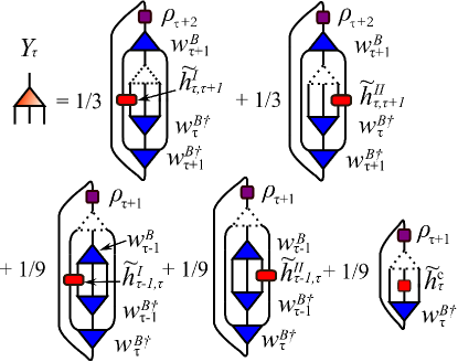
Figure 16: (Color online) The missing triangle corresponds $w^{B}_{\tau}$, and its corresponding environment $Y_{\tau}$ is defined by the sum of five tensor networks with certain weights.

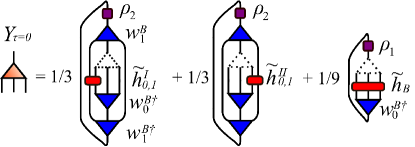
Figure 17: (Color online) The missing triangle corresponds to $w^{B}_{0}$, and its environment $Y_{0}$ includes three tensor networks, where the effective Hamiltonian $\widetilde{h}_{B}$ is defined in Fig. 5 (a).

Optimization in scale invariant layers– Similarly optimizing the central tensor of buffer layers in Eq. (39), one can define the corresponding environment to numerically obtain the scale invariant central tensors $w_{s}^{B}$. For the scale invariant layers, to find the optimal $w_{s}^{B}$, the cost function is defined as

$$E_{s} =tr\left\{w^{B}_{s}Y_{s}\right\},$$ (40)

where the corresponding environment $Y_{s}$ is a function of $w_{s}^{B}$, $w_{s}^{B\dagger}$, $\rho_{s}$, and $\widetilde{h}^{\nu}_{s}$ with $\nu\in I,II,{\rm c}$. The environment $Y_{s}$ is a weighted sum of tensor networks as shown in Fig. 18. We note that, however, at the first scale invariant layer, one should calculate the environment using Fig. 16 because the central tensor below is not $w^{B}_{s}$ but $w^{B}_{\tau_{bf-1}}$. This means that the environment of $w^{B}_{s}$ is distinct from that of $w^{B}_{\tau}$ for $\tau<\tau_{s}+1$. On the other hand, after the second scale invariant layer, the definition of the environment $Y_{s}$ in Fig. 18 is used, since all the next layers are characterized by the same tensor $w^{B}_{s}$.

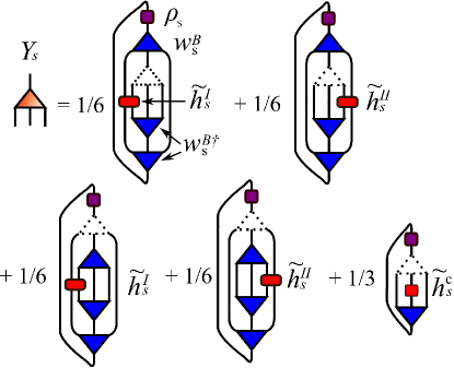
Figure 18: (Color online) Both the missing and the blue triangles represent the scale invariant central tensor $w^{B}_{s}$. The environment $Y_{s}$ is a sum of tensor networks composed of the scale invariant density matrix $\rho_{s}$ and the effective scale invariant Hamiltonian $\widetilde{h}_{s}^{\nu}$ with $\nu\in I,II,c$ defined in Eq. (17) and Eq. (41).

We here define a scale invariant central Hamiltonian,

$$\widetilde{h}^{\rm c}_{s} =\sum_{\tau=\tau^{\prime}_{s}}^{\infty}\frac{1}{3^{\tau-\tau^{\prime}_{s}}}\widetilde{h}_{\tau}^{\rm c}\;,$$ (41)

where $\tau$ starts from the third scale invariant layer $\tau^{\prime}_{s}=\tau_{s}+2$, and the construction of the central Hamiltonian $\widetilde{h}_{\tau}^{\rm c}$ is referred to Eq. (34). Moreover, from the numerical simulation perspective it is impossible to perform the infinite sum in Eq. (41); therefore, a cut-off of finite $L$ layers is introduced in the infinite sum. Due to the scale invariance, the two-site Hamiltonian $\widetilde{h}_{\tau,\tau+1}^{\mu}$ decays quickly as a power of $1/9$ when $\tau$ increases. Evenbly et al. (2010) Therefore, it is suitable to keep a finite number of $\widetilde{h}_{\tau,\tau+1}^{\mu}$

B.1 Algorithm of scale invariant boundary MERA

We briefly outline the overall update procedure for the central tensors in Fig. 13:

• Initialize $\widetilde{h}^{\rm c}_{\tau}$, $\widetilde{h}^{\mu}_{\tau,\tau+1}$, $\rho_{\tau}$, and $w^{B}_{\tau}$. The Hamiltonian $\widetilde{h}_{\tau,\tau+1}^{I}$ and $\widetilde{h}_{\tau,\tau+1}^{II}$ are obtained by the inhomogeneous coarse-graining in Eq. (33), and $\widetilde{h}_{\tau}^{\rm c}$ are carried out using the central ascending processes in Eq. (34) and in Eq. (35). For $\rho_{\tau}$ and $w^{B}_{\tau}$, we initialize them with the bulk tensors.

• Calculate the corresponding environment $Y_{\tau}$ of $w^{B}_{\tau}$ starting from the zeroth layer, and optimize $w^{B}_{\tau}$ by minimizing the cost function in Eq. (39). Iterative optimization is employed to acquire self-consistency for both $w^{B}_{\tau}$ and $Y_{\tau}$.

• Apply the average central ascending superoperator $\overline{A}$ to obtain the central Hamiltonian $\widetilde{h}_{\tau+1}^{\rm c}$ for the next layer.

• Go to Step 2 for the optimization of the next layer $(\tau+1)$ until the second scale invariant layer is reached.

• Apply the power method to obtain an optimal $\rho_{s}$. The scale invariant density matrix $\rho_{s}$ are the same for all the scale invariant layers.

• Calculate the effective scale invariant Hamiltonian $\widetilde{h}_{s}^{I},\widetilde{h}_{s}^{II}$ in Eq. (17), and $\widetilde{h}_{s}^{\rm c}$ in Eq. (41).

• Construct the scale invariant environment $Y_{s}$, optimize $w_{s}^{B}$ by Eq. (40).

• Apply the descending superoperator $D^{\rm c}$ on the density matrix from the top layer to the bottom and start over from Step 2.

This optimization procedure has several advantages. The most important is the feedback between the scale invariant layers and the buffer layers. The information of the entanglement is passed down from the scale invariant layer to the buffer layers by descending of the density matrix in Step 8. On the other hand, the feedback from the buffer layer to the scale invariant layer is achieved through $\widetilde{h}^{\rm c}_{s}$ by from the ascending of the boundary Hamiltonian and the central Hamiltonian. And when we optimize the central tensor $w^{B}_{s}$, we need to calculate $Y_{s}$ which contains the information of the effective scale invariant Hamiltonian. This optimization method is two-way feedback such that the RG flow can more quickly reach the fixed point.

Appendix C Correlation function with perfect transmission

With the attractive electron-electron interactions, i.e., Luttinger parameter $g>1$, the presence of a single impurity is renormalized to the situation as if the impurity is in absence. Kane and Fisher (1992a) Hence, all correction functions are the same as an infinite Luttinger liquid wire. In this Appendix, we will focus on the equal time current-current correlation function $\langle\mathcal{T}_{\tau}J^{\mu}(x)J^{\mu^{\prime}}(x)\rangle$ for $\mu\neq\mu^{\prime}$ corresponding to different wires.

From Eq. (13), we can decompose this correlation function by chiral currents as

$$\langle J^{\mu}(x)J^{\mu^{\prime}}(x)\rangle=-v^{2}\left(\langle\rho^{\mu}_{out}(x)\rho^{\mu^{\prime}}_{in}(x)\rangle+\langle\rho^{\mu}_{in}(x)\rho^{\mu^{\prime}}_{out}(x)\rangle\right).$$ (42)

Here, we omit the $\mathcal{T}_{\tau}$ symbol. As two LL wires connected by a weak link (impurity) behave the same as a single infinite LL wires for $g>1$, the chiral current correlation functions between two wires are given by

$$\langle\rho^{1}_{out}(x)\rho^{2}_{in}(x)\rangle=\langle\rho^{1}_{in}(x)\rho^{2}_{out}(x)=\frac{g}{4\pi^{2}}\frac{1}{(2x)^{2}}.$$ (43)

The normalization of the correlation function is followed by Eq. (7) and is consistent with Ref. Rahmani et al., 2012 The physical current-current correlation function is then given by

$$\langle J^{\mu}(x)J^{\mu^{\prime}}(x)\rangle=-\frac{v^{2}g}{8\pi^{2}}\frac{1}{x^{2}}.$$ (44)

This gives the exponent $\alpha=2$ and coefficient $A=\frac{v^{2}g}{8\pi^{2}}$ which we will benchmark against with our numerics.

References

- Joachim and Ratner (2005) C. Joachim and M. A. Ratner, PNAS 102, 8801 (2005).
- Ohshiro et al. (2012) T. Ohshiro, K. Matsubara, M. Tsutsui, M. F. M. Taniguchi, and T. Kawai, Scientific Reports 2 (2012), 10.1038/srep00501.
- Laroche et al. (2014) D. Laroche, G. Gervais, M. P. Lilly, and J. L. Reno, Science (2014), 10.1126/science.1244152.
- Ishii et al. (2003) H. Ishii, H. Kataura, H. Shiozawa, H. Yoshioka, H. Otsubo, Y. Takayama, T. Miyahara, S. Suzuki, Y. Achiba, M. Nakatake, T. Narimura, M. Higashiguchi, K. Shimada, H. Namatame, and M. Taniguchi, Nature 426, 540 (2003).
- Bockrath et al. (1999) M. Bockrath, D. H. Cobden, J. Lu, A. G. Rinzler, R. E. Smalley, L. Balents, and P. L. McEuen, Nature 397, 598 (1999).
- Yao et al. (1999) Z. Yao, H. W. C. Postma, L. Balents, and C. Dekker, Nature 402, 273 (1999).
- Kim et al. (2007) N. Y. Kim, P. Recher, W. D. Oliver, Y. Yamamoto, J. Kong, and H. Dai, Phys. Rev. Lett. 99, 036802 (2007).
- Postma et al. (2000) H. W. C. Postma, M. de Jonge, Z. Yao, and C. Dekker, Phys. Rev. B 62, R10653 (2000).
- Cardy (2010) J. L. Cardy, Conformal field theory and statistical mechanics, in J. Jacobsen et al. (eds), Exact Methods in Low-Dimensional Statistical Physics and Quantum Computing (Oxford University Press, Oxford, 2010).
- Affleck (2010) I. Affleck, Quantum impurity problems in condensed matter physics, in J. Jacobsen et al. (eds), Exact Methods in Low-Dimensional Statistical Physics and Quantum Computing (Oxford University Press, Oxford, 2010).
- Luttinger (1963) J. M. Luttinger, J. Math. Phys. 4, 1154 (1963).
- Kane and Fisher (1992a) C. L. Kane and M. P. A. Fisher, Phys. Rev. Lett. 68, 1220 (1992a).
- Kane and Fisher (1992b) C. L. Kane and M. P. A. Fisher, Phys. Rev. B 46, 15233 (1992b).
- Furusaki and Nagaosa (1993) A. Furusaki and N. Nagaosa, Phys. Rev. B 47, 4631 (1993).
- Wong and Affleck (1994) E. Wong and I. Affleck, Nucl. Phys. B 417, 403 (1994).
- Matveev et al. (1993) K. A. Matveev, D. Yue, and L. I. Glazman, Phys. Rev. Lett. 71, 3351 (1993).
- Affleck and Ludwig (1991) I. Affleck and A. Ludwig, Nucl. Phys. B 352, 849 (1991).
- Nayak et al. (1999) C. Nayak, M. P. A. Fisher, A. W. W. Ludwig, and H. H. Lin, Phys. Rev. B 59, 15694 (1999).
- Oshikawa et al. (2006) M. Oshikawa, C. Chamon, and I. Affleck, JSTAT 2006, P02008 (2006).
- Andergassen et al. (2004) S. Andergassen, T. Enss, V. Meden, W. Metzner, U. Schollwöck, and K. Schönhammer, Phys. Rev. B 70, 075102 (2004).
- Hamamoto et al. (2008) Y. Hamamoto, K.-I. Imura, and T. Kato, Phys. Rev. B 77, 165402 (2008).
- Freyn and Florens (2011) A. Freyn and S. Florens, Phys. Rev. Lett. 107, 017201 (2011).
- Barnabé-Thériault et al. (2005a) X. Barnabé-Thériault, A. Sedeki, V. Meden, and K. Schönhammer, Phys. Rev. B 71, 205327 (2005a).
- Barnabé-Thériault et al. (2005b) X. Barnabé-Thériault, A. Sedeki, V. Meden, and K. Schönhammer, Phys. Rev. Lett. 94, 136405 (2005b).
- Rahmani et al. (2010) A. Rahmani, C.-Y. Hou, A. Feiguin, C. Chamon, and I. Affleck, Phys. Rev. Lett. 105, 226803 (2010).
- Vidal (2007) G. Vidal, Phys. Rev. Lett. 99, 220405 (2007).
- Evenbly et al. (2010) G. Evenbly, R. N. C. Pfeifer, V. Picó, S. Iblisdir, L. Tagliacozzo, I. P. McCulloch, and G. Vidal, Phys. Rev. B 82, 161107 (2010).
- White (1992) S. R. White, Phys. Rev. Lett. 69, 2863 (1992).
- Schollwöck (2005) U. Schollwöck, Rev. Mod. Phys. 77, 259 (2005).
- Meden and Schollwöck (2003) V. Meden and U. Schollwöck, Phys. Rev. B 67, 193303 (2003).
- Rahmani et al. (2012) A. Rahmani, C.-Y. Hou, A. Feiguin, M. Oshikawa, C. Chamon, and I. Affleck, Phys. Rev. B 85, 045120 (2012).
- Karrasch and Moore (2012) C. Karrasch and J. E. Moore, Phys. Rev. B 86, 155156 (2012).
- Eggert and Affleck (1992) S. Eggert and I. Affleck, Phys. Rev. B 46, 10866 (1992).
- Qin et al. (1996) S. Qin, M. Fabrizio, and L. Yu, Phys. Rev. B 54, R9643 (1996).
- Enss et al. (2005) T. Enss, V. Meden, S. Andergassen, X. Barnabé-Thériault, W. Metzner, and K. Schönhammer, Phys. Rev. B 71, 155401 (2005).
- Andergassen et al. (2006) S. Andergassen, T. Enss, V. Meden, W. Metzner, U. Schollwöck, and K. Schönhammer, Phys. Rev. B 73, 045125 (2006).
- Evenbly and Vidal (2009) G. Evenbly and G. Vidal, Phys. Rev. B 79, 144108 (2009).
- Pfeifer et al. (2009) R. N. C. Pfeifer, G. Evenbly, and G. Vidal, Phys. Rev. A 79, 040301 (2009).
- Evenbly and Vidal (2013a) G. Evenbly and G. Vidal, (2013a), arXiv:1312.0303 .
- Weng (2010) M. Q. Weng, EPL (Europhysics Letters) 92, 60005 (2010).
- Silvi et al. (2010) P. Silvi, V. Giovannetti, P. Calabrese, G. E. Santoro, and R. Fazio, Journal of Statistical Mechanics: Theory and Experiment 2010, L03001 (2010).
- Cardy and Lewellen (1991) J. L. Cardy and D. C. Lewellen, Phys. Lett. B 259, 274 (1991).
- Evenbly and Vidal (2013b) G. Evenbly and G. Vidal, (2013b), arXiv:1307.0831 .
- Avella and Mancini (2013) A. Avella and F. Mancini, Strongly Correlated Systems, Springer Series in Solid-State Sciences, Vol. 176 (Springer, 2013).
- Lukyanov (1998) S. Lukyanov, Nuclear Physics B 522, 533 (1998).
- Lukyanov and Terras (2003) S. Lukyanov and V. Terras, Nuclear Physics B 654, 323 (2003).
- Lal et al. (2002) S. Lal, S. Rao, and D. Sen, Phys. Rev. B 66, 165327 (2002).
- Chen et al. (2002) S. Chen, B. Trauzettel, and R. Egger, Phys. Rev. Lett. 89, 226404 (2002).
- Egger et al. (2003) R. Egger, B. Trauzettel, S. Chen, and F. Siano, New Journal of Physics 5, 117 (2003).
- Pham et al. (2003) K.-V. Pham, F. Piéchon, K.-I. Imura, and P. Lederer, Phys. Rev. B 68, 205110 (2003).
- Kazymyrenko and Doucot (2005) K. Kazymyrenko and B. Doucot, Phys. Rev. B 71, 075110 (2005).
- Das and Rao (2008) S. Das and S. Rao, Phys. Rev. B 78, 205421 (2008).
- Bellazzini et al. (2009) B. Bellazzini, M. Mintchev, and P. Sorba, Phys. Rev. B 80, 245441 (2009).
- Aristov et al. (2010) D. N. Aristov, A. P. Dmitriev, I. V. Gornyi, V. Y. Kachorovskii, D. G. Polyakov, and P. Wolfle, Phys. Rev. Lett. 105, 266404 (2010).
- Aristov (2011) D. N. Aristov, Phys. Rev. B 83, 115446 (2011).
- Aristov and Wölfle (2011) D. N. Aristov and P. Wölfle, Phys. Rev. B 84, 155426 (2011).
- Hou and Chamon (2008) C.-Y. Hou and C. Chamon, Phys. Rev. B 77, 155422 (2008).
- Safi and Schulz (1995) I. Safi and H. J. Schulz, Phys. Rev. B 52, R17040 (1995).
- Maslov and Stone (1995) D. L. Maslov and M. Stone, Phys. Rev. B 52, R5539 (1995).
- Aristov and Wölfle (2012) D. N. Aristov and P. Wölfle, Phys. Rev. B 86, 035137 (2012).
- Hou et al. (2012) C.-Y. Hou, A. Rahmani, A. E. Feiguin, and C. Chamon, Phys. Rev. B 86, 075451 (2012).
- Aristov and Wölfle (2013) D. N. Aristov and P. Wölfle, Phys. Rev. B 88, 075131 (2013).
- Cirillo et al. (2011) A. Cirillo, M. Mancini, D. Giuliano, and P. Sodano, Nuclear Physics B 852, 235 (2011).
- Giuliano and Sodano (2013) D. Giuliano and P. Sodano, EPL (Europhysics Letters) 103, 57006 (2013).