Aspiration Dynamics of Multi-player Games in Finite Populations

Abstract

Studying strategy update rules in the framework of evolutionary game theory, one can differentiate between imitation processes and aspiration-driven dynamics. In the former case, individuals imitate the strategy of a more successful peer. In the latter case, individuals adjust their strategies based on a comparison of their payoffs from the evolutionary game to a value they aspire, called the level of aspiration. Unlike imitation processes of pairwise comparison, aspiration-driven updates do not require additional information about the strategic environment and can thus be interpreted as being more spontaneous. Recent work has mainly focused on understanding how aspiration dynamics alter the evolutionary outcome in structured populations. However, the baseline case for understanding strategy selection is the well-mixed population case, which is still lacking sufficient understanding. We explore how aspiration-driven strategy-update dynamics under imperfect rationality influence the average abundance of a strategy in multi-player evolutionary games with two strategies. We analytically derive a condition under which a strategy is more abundant than the other in the weak selection limiting case. This approach has a long standing history in evolutionary game and is mostly applied for its mathematical approachability. Hence, we also explore strong selection numerically, which shows that our weak selection condition is a robust predictor of the average abundance of a strategy. The condition turns out to differ from that of a wide class of imitation dynamics, as long as the game is not dyadic. Therefore a strategy favored under imitation dynamics can be disfavored under aspiration dynamics. This does not require any population structure thus highlights the intrinsic difference between imitation and aspiration dynamics.

1 Introduction

In the study of population dynamics, it turns out to be very useful to classify individual interactions in terms of evolutionary games [1]. Early mathematical theories of strategic interactions were based on the assumption of rational choice [2, 3]: an agent’s optimal action depends on its expectations on the actions of others, and each of the other agents’ actions depend on their expectations about the focal agent. In evolutionary game theory, successful strategies spread by reproduction or imitation in a population [4, 5, 6, 7, 8].

Evolutionary game theory not only provides a platform for explaining biological problems of frequency dependent fitness and complex individual interactions such as cooperation and coordination [9, 10]. In finite populations, it also links the neutral process of evolution [11] to frequency dependence by introducing an intensity of selection [12, 13, 14, 15]. Evolutionary game theory can also be used to study cultural dynamics including human strategic behavior and updating [16, 17, 18]. One of the most interesting open questions is How do individuals update their strategies based on the knowledge and conception of others and themselves?

Two fundamentally different mechanisms can be used to classify strategy updating and population dynamics based on individuals’ knowledge about their strategic environment or themselves: imitation of others and self-learning based on one’s own aspiration. In imitation dynamics, players update their strategies after a comparison between their own and another individual’s success in the evolutionary game [19, 20, 21]. For aspiration-driven updating, players switch strategies if an aspiration level is not met, where the level of aspiration is an intrinsic property of the focal individual [22, 23, 24, 25]. In both dynamics, novel strategies cannot emerge without additional mechanisms such as spontaneous exploration of strategy space (similar to mutation) [26, 27, 19, 28, 29, 30]. The major difference is that the latter does not require any knowledge about the payoffs of others. Thus aspiration level based dynamics, a form of self-learning, require less information about an individual’s strategic environment than imitation dynamics.

Aspiration-driven strategy-update dynamics are commonly observed in studies of animal and human behavioral ecology. For example, fish would ignore social information when they have relevant personal information [31], and experienced ants hunt for food based on their own previous chemical trials rather than imitating others [32]. Furthermore, a form of aspiration-level-driven dynamics play a key role in the individual behaviors in rat populations [33]. These examples clearly show that the idea behind aspiration dynamics, i.e., self-evaluation, is present in the animal world. In behavioral sciences, such aspiration-driven strategy adjustments generally operate on the behavioral level. However, it can be speculated that self-learning processes can have such an effect that it might actually have a downward impact on regulatory, and thus genetic levels of brain and nervous system. This, in turn, could be seen as a mechanism that alters the rate of genetic change [34]. Whereas such wide reaching systemic alterations are more speculative, it is clear that aspiration levels play a role in human strategy updating [23].

We study the statistical mechanics of a simple case of aspiration-driven self-learning dynamics in well-mixed populations of finite size. Deterministic and stochastic models of imitation dynamics have been well studied in both well-mixed and structured populations [6, 35, 26, 24, 19, 36]. For aspiration dynamics, numerous works have emerged studying population dynamics on graphs, but its impact in well-mixed populations–a basic reference case, one would think–is far less well understood. Although deterministic aspiration dynamics, i.e., a kind of win-stay-lose-shift dynamics, in which individuals are perfectly rational have been analyzed [37], it is not clear how processes with imperfect rationality influence the evolutionary outcome. Here, we ask whether a strategy favored under pairwise comparison driven imitation dynamics can become disfavored under aspiration-driven self-learning dynamics. To this end, in our analytical analysis, we limit ourselves to the weak selection, or weak rationality approximation, where payoffs via the game play little role in the decision-making [35]. As it has been shown that under weak selection, the favored strategy is invariant for a wide class of imitation processes [27, 21, 38]. We show that for pairwise games, the aspiration dynamics and the imitation dynamics always share the same favored strategies. For multi-player games, however, the weak selection criterion under aspiration dynamics that determines whether a strategy is more abundant than the other differs from the criterion under imitation dynamics. This paves the way to construct multi-player games, for which aspiration dynamics favor one strategy whereas imitation dynamics favor another. Furthermore, in contrast to deterministic aspiration dynamics, if the favored strategy is determined by a global aspiration level, the average abundance of a strategy in the stochastic aspiration dynamics is invariant with respect to the aspiration level, provided selection is weak. We also extrapolate our results to stronger selection cases through numerical simulation.

2 Mathematical Model

2.1 Evolutionary games

We consider evolutionary game dynamics with two strategies and $d$ players. From these, the more widely studied $2\times 2$ games emerge as a special case [36]. In individual encounters, players obtain their payoffs from simultaneous actions. A focal player can be of type $A$, or $B$, and encounter a group containing $k$ other players of type $A$, to receive the payoff $a_{k}$, or $b_{k}$. For example, a $B$ player, which encounters $d-1$ individuals of type $A$, obtains payoff $b_{d-1}$. An $A$ player in a group of one other $A$ player and thus $d-2$ $B$ players obtains payoff $a_{1}$. All possible payoffs of a focal individual are uniquely defined by the number of $A$ in the group, such that the payoff matrix reads

(2.4)

For any group engaging in a one-shot game, we can obtain each member’s payoff according to this matrix.

In a finite well-mixed population of size $N$, groups of size $d$ are assembled randomly, such that the probability of choosing a group that consists of another $k$ players of type $A$, and of $d-1-k$ players of type $B$, is given by a hypergeometric distribution [39]. For example, the probability that an $A$ player is in a group of $k$ other $A$s is given by $\text{prob}_{A}(\,k\,|\,N,i,d\,)=(\,C_{i-1}^{k}\,C_{N-i}^{d-1-k}\,)/C_{N-1}^{d-1}$, where $i$ ($i\geq d$) is the number of $A$ players in the population, and $C^{k}_{n}=n!/(\,k!\,(n-k)!\,)$ is the binomial coefficient.

The expected payoffs for any $A$ or $B$ in a population of size $N$, with $i$ players of type $A$ and $N-i$ players of type $B$, are given by

$$\pi_{A}(i) =\sum_{k=0}^{d-1}\frac{C_{i-1}^{k}\,C_{N-i}^{d-1-k}}{C_{N-1}^{d-1}}\,a_{k},$$ (2.5)

$$\pi_{B}(i) =\sum_{k=0}^{d-1}\frac{C_{i}^{k}\,C_{N-i-1}^{d-1-k}}{C_{N-1}^{d-1}}\,b_{k}.$$ (2.6)

In summary, we define a $d$-player stage game [7], shown in Eq. (2.4), from which the evolutionary game emerges such that each individual obtains an expected payoff based on the current composition of the well-mixed population. In the following, we introduce an update rule based on a global level of aspiration. This allows us to define a Markov chain describing the inherently stochastic dynamics in a finite population: probabilistic change of the composition of the population is driven by the fact that each individual compares its actual payoff to an imaginary value that it aspires. Note here that we are only interested in the simplest way to model such a complex problem and do not address any learning process that may adjust such an aspiration level as the system evolves. For a sketch of the aspiration-driven evolutionary game, see Fig. 1.

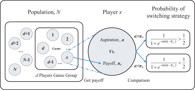
Figure 1: Evolutionary game dynamics of $d$-player interactions driven by global aspiration. In our mathematical model of human strategy updating driven by self-learning, a group of $d$ players is chosen randomly from the finite population to play the game. According to this, game players calculate and obtain their actual payoffs. They are more likely to stochastically switch strategies if the payoffs they aspire are not met. On the other hand, the higher the payoffs compared to the aspiration level $\alpha$ are, the less likely they switch their strategies. Besides, strategy switching is also determined by a selection intensity $\omega$. For vanishing selection intensity, switching is entirely random irrespective of payoffs and the aspiration level. For increasing selection intensity, the self-learning process becomes increasingly more “optimal” in the sense that for high $\omega$, individuals tend to always switch when they are dissatisfied, and never switch when they are tolerant. We examine the simplest possible setup, where the level of aspired payoff $\alpha$ is a global parameter that does not change with the dynamics. We show that, however, statements about the average abundance of a strategy do not depend on $\alpha$ under weak selection ($\omega\ll 1$).

2.2 Aspiration-level driven stochastic dynamics

In addition to the inherent stochasticity in finite populations, there is randomness in the process of individual assessments of one’s own payoff as compared to a random sample of the rest of the population; even if an individual knew exactly what to do, he might still fail to switch to an optimal strategy, e.g., due to a trembling hand [40, 41].

Here we examine the simplest case of an entire population having a certain level of aspiration. Players needn’t see any particular payoffs but their own, which they compare to an aspired value. This level of aspiration, $\alpha$, is a variable that influences the stochastic strategy updating. The probability of switching strategy is random when individuals’ payoffs are close to their level of aspiration, reflecting the basic degree of uncertainty in the population. When payoffs exceed the aspiration, strategy switching is unlikely. At high values of aspiration compared to payoffs, switching probabilities are high.

The level of aspiration provides a global benchmark of tolerance or dissatisfaction in the population. In addition, when modeling human strategy updating, one typically introduces another global parameter that provides a measure for how important individuals deem the impact of the actual game played on their update, the intensity of selection, $\omega$. Irrespective of the aspiration level and the frequency dependent payoff distribution, vanishing values of $\omega$ refer to nearly random strategy updating. For large values of $\omega$, individuals’ deviations from their aspiration level have a strong impact on the dynamics.

Note that although the level of aspiration is a global variable and does not differ individually, due to payoff inhomogeneity there can always be a part of the population that seeks to switch more often due to dissatisfaction with the payoff distribution.

In our microscopic update process, we randomly choose an individual, $x$, from the population, and assume that the payoff of the focal individual is $\pi_{x}$. To model stochastic self-learning of aspiration-driven switching, we can use the following probability function

$$g(\,\alpha-\pi_{x}\,)=\frac{1}{1+e^{-\omega\,(\,\alpha-\pi_{x}\,)}},$$ (2.7)

which is similar to the Fermi-rule [42, 22], but replaces a randomly drawn opponent’s payoff by one’s own aspiration. The wider the positive gap between aspiration and payoff, the higher the switching probability. Reversely, if payoffs exceed the level of aspiration individuals become less active with increasing payoffs. The aspiration level, $\alpha$, provides the benchmark used to evaluate how “greedy” an individual is. Higher aspiration levels mean that individuals aspire to higher payoffs. If payoffs meet aspiration, individuals remain random in their updates. If payoffs are below aspiration, switching occurs with probability larger than random; if they are above aspiration, switching occurs with probability lower than random. The selection intensity governs how strict individuals are in this respect. For $\omega=0$, strategy switching is entirely random (neutral). Low values of $\omega$ lead to switching only slightly different from random but follow the impact of $\alpha$. For increasing $\omega$, the impact of the difference between payoffs and the aspiration becomes more important. In the case of $\omega\to\infty$, individuals are strict in the sense that they either switch strategies with probability one if they are not satisfied, or stay with their current strategy if their aspiration level is met or overshot.

The spread of successful strategies is modeled by a birth and death process in discrete time. In one time step, three events are possible: the abundance of $A$, $i$, can increase by one with probability $p(\,i\to i+1\,)=T_{i}^{+}$, decrease by one with probability $p(\,i\to i-1\,)=T_{i}^{-}$, or stay the same with probability $p(\,i\to i\,)=T_{i}^{0}$. All other transitions occur with probability zero. The transition probabilities are given by

$$T_{i}^{+} =\frac{N-i}{N}\,\frac{1}{1+e^{-\omega\,[\,\alpha-\pi_{B}(i)\,]}},$$ (2.8)

$$T_{i}^{-} =\frac{i}{N}\,\frac{1}{1+e^{-\omega\,[\,\alpha-\pi_{A}(i)\,]}},$$ (2.9)

$$T_{i}^{0} =1-T_{i}^{+}-T_{i}^{-}.$$ (2.10)

In each time step, a randomly chosen individual evaluates its success in the evolutionary game, given by Eqs. (2.5), (2.6), compares it to the level of aspiration, and then changes strategy with probability lower than $1/2$ if its payoff exceeds the aspiration. Otherwise, it switches with probability greater than $1/2$, except when the aspiration level is exactly met, in which case it switches randomly (note that this is very unlikely to ever be the case).

Compared to imitation (pairwise comparison) dynamics, our self-learning process, which is essentially an Ehrenfest-like Markov chain, has some different characteristics. Without the introduction of mutation or random strategy exploration, there exists a stationary distribution for the aspiration-driven dynamics. Even in a homogenous population, there is a positive probability that an individual can switch to another strategy due to the dissatisfaction resulting from payoff-aspiration difference. This facilitates the escape from the states that are absorbing in the pairwise comparison process and other Moran-like evolutionary dynamics. Hence there exists a nontrivial stationary distribution of the Markov chain satisfying detailed balance. Specifically, for the case of $\omega=0$ (neutral selection), the dynamics defined by Eqs. (2.8)–(2.10) are characterized by linear rates, while these rates are quadratic for the neutral imitation dynamics and Moran process.

In the following analysis and discussion, we are interested in the limit of weak selection, $\omega\ll 1$, and its ability to aptly predict the success of cooperation in commonly used evolutionary $d-$player games. The limit of weak selection, which has a long standing history in population genetics and molecular evolution [11] also plays a role in social learning and cultural evolution. Recent experimental results suggest that the intensity with which human subjects adjust their strategies might be low [18]. Although it has been unclear to what degree and in what way human strategy updating deviates from random [43, 44], the weak selection limit is of importance to quantitatively characterize the evolutionary dynamics. In the limiting case of weak selection, we are able to analytically classify strategies with respect to the neutral benchmark, $\omega\to 0$ [35, 19, 45, 21, 46]. We note that a strategy is favored by selection, if its average equilibrium frequency under weak selection is greater than one half. In order to come to such a quantitative observation, we need to calculate the stationary distribution over frequencies of strategy $A$.

2.3 Stationary distribution

The Markov chain given by Eqs. (2.8)–(2.10) is a one dimensional birth and death process with reflecting boundaries. It satisfies the detailed balance condition $\psi_{j-1}\,T_{j-1}^{+}=\psi_{j}\,T_{j}^{-}$, where

$$(\,\psi_{0},\psi_{1},\dots,\psi_{j},\dots,\psi_{N}\,)$$

is the stationary distribution over frequencies of $A$ in equilibrium [47, 48]. Considering $\sum_{j=0}^{N}\psi_{j}=1$, we find the exact solution by recursion, given by

$$\psi_{j}=\begin{cases}j=0:\,\,\,\frac{1}{1+\sum_{k=1}^{N}q_{0\,k-1}^{+}/q_{1\,k}^{-}}\\ \\ j>0:\,\,\,\frac{q_{0\,j-1}^{+}/q_{1\,j}^{-}}{1+\sum_{k=1}^{N}q_{0\,k-1}^{+}/q_{1\,k}^{-}}\end{cases},$$ (2.11)

where $q_{j\,k}^{\pm}=\prod_{l=j}^{k}T_{l}^{\pm}$ is the probability of successive transitions from $j$ to $k$. The analytical solution Eq. (2.11) allows us to find the exact value of the average abundance of strategy $A$,

$$\langle X_{A}\rangle(\omega)=\sum_{j=0}^{N}\frac{j}{N}\,\psi_{j}(\omega),$$ (2.12)

for any strength of selection.

3 Results and Discussion

It has been shown that imitation processes are similar to each other under weak selection [27, 21, 38]. Thus in order to compare the essential differences between imitation processes and aspiration process, we consider such selection limit. To better understand the effects of selection intensity, aspiration level, and payoff matrix on the average abundance of strategy $A$, we further analyze which strategy is more abundant based on Eq. (2.11). For a fixed population size, under weak selection, i.e. $\omega\rightarrow 0$, the stationary distribution $\psi_{j}(\omega)$ can be expressed approximately as

$$\psi_{j}(\omega)\approx\psi_{j}(0)+\omega\,\left[\,\frac{\partial}{\partial\,\omega}\,\psi_{j}(\omega)\,\right]_{\omega=0},$$ (3.1)

where the neutral stationary distribution is simply given by $\psi_{j}(0)=C_{N}^{j}/2^{N}$, and the first order term of this Taylor expansion amounts to

$$\left[\,\frac{\partial}{\partial\,\omega}\,\psi_{j}(\omega)\,\right]_{\omega=0}=\frac{C_{N}^{j}}{2^{N+1}}\,\left\{\sum\limits_{k=1}^{j}[\,\pi_{A}(k)-\pi_{B}(k-1)\,]-\frac{1}{2^{N}}\,\sum\limits_{k=1}^{N}\,C_{N}^{k}\sum\limits_{l=1}^{k}[\,\pi_{A}(l)-\pi_{B}(l-1)\,]\right\}.$$ (3.2)

Interestingly, in the limiting case of weak selection, the first order approximation of the stationary distribution of $A$ does not depend on the aspiration level. For higher order terms of selection intensity, however, $\psi_{j}(\omega)$ does depend on the aspiration level.

In the following we discuss the condition under which a strategy is favored and compare the predictions for stationary strategy abundance under self-learning and under imitation dynamics. Thereafter we consider three prominent examples of games with multiple players through analytical, numerical and simulation methods, the results of which are detailed in Figs. 2–4 and Appendix B. All three examples are social dilemmas in the sense that the Nash equilibrium of the one-shot game is not the social optimum. First, the widely studied public goods game represents the class of games where there is only one pure Nash equilibrium [49]. Next, the public goods game with a threshold, a simplified version of the collective risk dilemma [50, 51, 52], represents the class of coordination games with multiple pure Nash equilibria, depending on the threshold. Last, we consider the $d$-player volunteer’s dilemma, or snowdrift game, which has a mixed Nash equilibrium [53, 54].

3.1 Average abundance of strategy $A$

Based on the approximation (3.1), for any symmetric multi-player game with two strategies of normal form (2.4), we can now calculate a weak selection condition such that in equilibrium $A$ is more abundant than $B$. Since for neutrality, $\psi_{j}(0)=C_{N}^{j}/2^{N}$ holds and thus $\langle X_{A}\rangle(0)=1/2$, it is sufficient to consider positivity of the sum of $j\omega\,[\,\partial_{\omega}\,\psi_{j}(\omega)\,]_{\omega=0}/N$ over all $j=0,\dots,N$. Under weak selection, strategy $A$ is favored by selection, i.e., $\langle X_{A}\rangle(\omega)>1/2$, if

$$\sum_{k=0}^{d-1}C_{d-1}^{k}\left(\,a_{k}-b_{k}\,\right)>0,$$ (3.3)

which holds for any $d$-player games with two strategies in a population with more than two individuals. For a detailed derivation of our main analytical result, see Appendix A. Note that for a two-player game, $d=2$, the above condition simplifies to $a_{1}+a_{0}>b_{1}+b_{0}$, which is similar to the concept of risk-dominance translated to finite populations [35].

The left hand side expression of inequality (3.3) can also be compared to a similar condition under the class of pairwise comparison processes [22, 19], where two randomly selected individuals compare their payoffs and switch with a certain probability based on the observed inequality. Typically, weak selection results for pairwise comparison processes lead to the result that strategy $A$ is favored by selection if [55, 56, 35]

$$\sum_{k=0}^{d-1}\left(\,a_{k}-b_{k}\,\right)>0,$$ (3.4)

which applies both, to evaluate whether fixation of $A$ is more likely than fixation of $B$, or whether the average abundance of $A$ is greater than one half under weak mutation and weak selection, that can be shown using properties of the embedded Markov chain [57]. The sums on the left hand sides of (3.3) and (3.4) can thus be compared with each other in order to reveal the nature of our self-learning process driven by a global aspiration level.

Our main result, Eq. (3.3), holds for a variety of self-learning dynamics, not only for the probability function given by Eq. (2.7). Considering the general self-learning function $g[\,\omega\,(\,\alpha-\pi_{x}\,)\,]$ with $g(0)\neq 0$, here $g(x)$ is strictly increasing with increasing $x$. Denoting $u=\omega\,(\,\alpha-\pi_{x}\,)$, we have $g^{\prime}(\omega)=g^{\prime}(u)\,u^{\prime}(\omega)$. Then, for $\omega\rightarrow 0$, $\left.g^{\prime}(\omega)\right|_{\omega=0}=g^{\prime}(0)\,(\,\alpha-\pi_{x}\,)$, and Eq. (3.2) can be rewritten in a more general form

$$\left[\,\frac{\partial}{\partial\,\omega}\,\psi_{j}(\omega)\,\right]_{\omega=0}=\frac{g^{\prime}(0)}{g(0)}\,\frac{C_{N}^{j}}{2^{2N}}\,\left\{2^{N}\,\sum_{k=1}^{j}[\,\pi_{A}(k)-\pi_{B}(k-1)\,]-\sum_{k=1}^{N}\,C_{N}^{k}\sum_{i=1}^{k}[\,\pi_{A}(i)-\pi_{B}(i-1)\,]\right\}.$$ (3.5)

Since $g^{\prime}(0)/g(0)$ is a positive constant, Eq. (3.3) is still valid for any such probability function $g(x)$, see Appendix A.

3.2 Linear public goods game

Public goods games emerge when groups of players engage in the sustenance of common goods. Cooperators $A$ pay an individual cost in form of a contribution $c$ that is pooled into the common pot. Defectors $B$ do not contribute. The pot is then multiplied by a characteristic multiplication factor $r$ and shared equally among all individuals in the group, irrespective of contribution. If the multiplication factor is smaller than the size of the group $d$, each cooperator recovers only a fraction of the initial investment. Switching to defection would always be beneficial in a pairwise comparison of the two strategies. The payoff matrix thus reads

(3.9)

where $1<r<d$ is typically assumed. Since $a_{k}-b_{k}=c\,(r/d-1)$ is a negative constant for any number of cooperators in the group, we find that

$$\sum_{k=0}^{d-1}C_{d-1}^{k}\,(\,a_{k}-b_{k}\,)=2^{d-1}\,c\,\left(\,\frac{r}{d}-1\,\right)$$ (3.10)

is always negative. Cooperation cannot be the more abundant strategy in the well-mixed population (see Fig. 2). However, if the self-learning dynamics are driven by a sufficiently high aspiration level, individuals are constantly dissatisfied and switch strategy frequently, even as defectors, such that cooperation can break even if selection is strong enough, namely $\lim_{\alpha\to\infty}\langle X_{A}\rangle=1/2$ for all values $\omega$. On the other hand, if the aspiration level is low, cooperators switch more often than defectors such that the average abundance of $A$ assumes a value closer to the evolutionary stable state of full defection, which depends on $\omega$. In the extreme case of very low $\alpha$ and strong selection, defectors fully dominate, thus the stationary measure retracts to the all defection state.

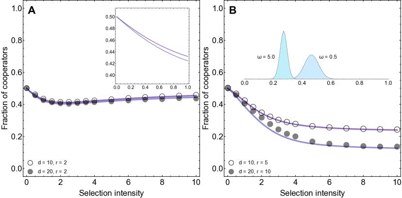
Figure 2: Mean (stationary) fraction of cooperators for the linear public goods game. The common parameters are aspiration level $\alpha=1$, population size $N=100$, and cost of cooperation $c=1$. In both panels, the group sizes are $d=10$ (dark shaded), and $d=20$ (light shaded). Panel A shows the mean fraction of cooperators as a function of selection intensity for $r=2$, the inset shows a detail for lower selection intensities. Panel B shows the mean fraction of cooperators as a function of selection intensity for $r=d/2$. The inset shows the stationary distribution for $d=10$, $r=5$ and $\omega=0.5,\,5$.

3.3 Threshold public goods game

Here we consider the following public goods game with a threshold in the sense that the good becomes strictly unavailable when the number of cooperators in a group is below a critical threshold, $m$. This threshold becomes a new strategic variable. Here, $c$ is an initial endowment given to each player, which is invested in full by cooperators. Whatever the cooperators manage to invest is multiplied by $r$ and redistributed among all players in the group irrespective of strategy, if the threshold investment $m\,c$ is met. Defectors do not make any investment, and thus have an additional payoff of $c$, as long as the threshold is met. Once the number of cooperators is below $m$, all payoffs are zero, which compares to the highest risk possible (loss of endowment and investment with certainty) in what is called the collective-risk dilemma [50, 52]. The payoff matrix for the two strategies, cooperation $A$, and defection $B$, reads

(3.14)

We can examine when the self-learning process favors cooperation. We can also seek to make a statement about whether under self-learning dynamics, cooperation performs better than under pairwise comparison process. For self-learning dynamics, we find

$$\sum_{k=0}^{d-1}C_{d-1}^{k}\,(\,a_{k}-b_{k}\,)=\sum_{k=m}^{d-1}C_{d-1}^{k}\,(\,r\,c/d-c\,)+C_{d-1}^{m-1}\,(\,m\,r\,c/d\,)$$

while the equivalent statement for pairwise comparison processes based on the same payoff matrix would be $\sum_{k=0}^{d-1}(\,a_{k}-b_{k}\,)=c\,(\,r+m-d\,)$. Thus, the criterion of self-learning dynamics can be written as

$$r>(\,d\,\sum_{k=m}^{d-1}C_{d-1}^{k})/(\,\sum_{k=m}^{d-1}C_{d-1}^{k}+m\,C_{d-1}^{m-1}\,)$$

whereas positivity of the imitation processes condition, $\sum_{k=0}^{d-1}(\,a_{k}-b_{k}\,)>0$, simply leads to $r>d-m$. Comparing the two conditions, we find

$$(\,d-m\,)-\frac{d\,\sum_{k=m}^{d-1}C_{d-1}^{k}}{\sum_{k=m}^{d-1}C_{d-1}^{k}+m\,C_{d-1}^{m-1}}=\frac{m}{\sum_{k=m}^{d-1}C_{d-1}^{k}+m\,C_{d-1}^{m-1}}\,\Gamma_{d,m}.$$ (3.15)

Since the first factor on the right hand side of Eq. (3.15) is always positive, the factor

$$\Gamma_{d,m}=(\,d-m\,)\,C_{d-1}^{m-1}-\sum_{k=m}^{d-1}C_{d-1}^{k}$$ (3.16)

determines the relationship between self-learning dynamics and pairwise comparison processes: for sufficiently large threshold $m$, expression (3.16) is positive. In conclusion, the aspiration-level-driven self-learning dynamics can afford to be less strict than the pairwise comparison process. Namely, it requires less reward for cooperators’ contribution to the common pool (lower levels of $r$) in order to promote the cooperative strategy. The amount of cooperative strategy depends on the threshold: higher thresholds support cooperation, even for lower multiplication factors $r$ (see Fig. 3). For fixed $r$, our self-learning dynamics are more likely to promote cooperation in a threshold public goods game, if the threshold for the number of cooperators needed to support the public goods is large enough, i.e., not too different from the total size of the group. For small thresholds, and thus higher temptation to defect in groups with less cooperators, we approach the regular public goods games, and the conclusion may be reversed. Under such small $m$ cases, imitation-driven (pairwise comparison) dynamics are more likely to lead to cooperation than aspiration dynamics.

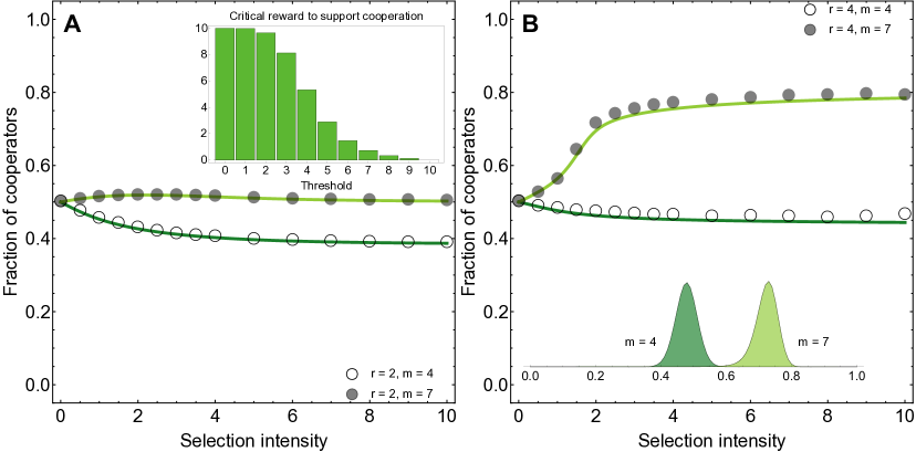
Figure 3: Mean (stationary) fraction of cooperators for the threshold public goods game. The common parameters are aspiration level $\alpha=1$, population size $N=100$, group size $d=10$, and cost of cooperation $c=1$. In both panels, the threshold sizes are $m=4$ (dark shaded), and $m=7$ (light shaded). Panel A shows the mean fraction of cooperators as a function of selection intensity for $r=2$. The inset shows the critical multiplication factor above which cooperation is more abundant as a function of the threshold $m$. High thresholds lower the critical multiplication factor of the public good such that cooperation can become more abundant than defection. Panel B shows the mean fraction of cooperators as a function of selection intensity for $r=4$. The inset shows the stationary distribution for $d=10$, $r=4$, $\omega=2$, and $m=4,\,7$.

3.4 $d$-player snowdrift game

Evolutionary games between two strategies can have mixed evolutionary stable states [6, 36]. Strategy $A$ can invade $B$ and $B$ can invade $A$; a stable coexistence of the two strategies typically evolves. In the replicator dynamics of the snowdrift game, cooperators can be invaded by defectors as the temptation to defect is still larger than the reward of mutual cooperation [54, 58]. In contrast to the public goods game, cooperation with a group of defectors now yields a payoff greater than exclusive defection. The act of cooperation provides a benefit to all members of the group, and the cost of cooperation is equally shared among the number of cooperators [59]. Hence, the payoff matrix reads

(3.20)

Cooperation can maintain a minimal positive payoff from the cooperative act, then cooperation and defection can coexist. The snowdrift game is a social dilemma, as selection does not favor the social optimum of exclusive cooperation. The level of coexistence depends on the amount of cost that a particular cooperator has to contribute in a certain group. Evaluating the weak selection condition, (3.3) in case of the $d$-player snowdrift game leads to the condition

$$\sum_{k=0}^{d-1}\frac{C_{d-1}^{k}}{k+1}<\frac{b}{c}$$ (3.21)

in order to observe $\langle X_{A}\rangle>1/2$ in aspiration dynamics under weak selection. For imitation processes, on the other hand, we find $\sum_{k=0}^{d-1}1/(k+1)<b/c$. Note that, except for $a_{0}-b_{0}=b-c>0$, $a_{k}-b_{k}<0$ holds for any other $k$. Because of this, the different nature of these two conditions, given by the positive coefficients $C_{d-1}^{k}>1$ for any $d>k>0$, reveals that self-learning dynamics narrow down the parameter range for which cooperation can be favored by selection. In the snowdrift game, self-learning dynamics are less likely to favor cooperation than pairwise comparison processes. Larger group size $d$ hinders cooperation: the larger the group, the higher the benefit of cooperation, $b$, has to be in order to support cooperation (see Fig. 4).

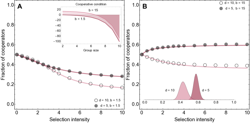
Figure 4: Mean (stationary) fraction of cooperators for the $d$-player snowdrift game. The common parameters are aspiration level $\alpha=1$, population size $N=100$, and cost of cooperation $c=1$. In both panels, the group sizes are $d=5$ (dark shaded), and $d=10$ (light shaded). Panel A shows the mean fraction of cooperators as a function of selection intensity for $b=1.5$. The inset shows the cooperation condition as a function of group size $d$ for benefits $b=1.5,\,15.0$. Only for high benefit and low group size, cooperation can be more abundant than defection. Panel B shows the mean fraction of cooperators as a function of selection intensity for $b=15.0$. The inset shows the stationary distribution for $b=15.0$, $\omega=2$, and $d=5,\,10$.

4 Summary and Conclusions

Previous studies on self-learning mechanism have typically been investigated on graphs via simulations, which often employ stochastic aspiration-driven update rules [60, 61, 25, 62, 23]. Although results based on the mean field approximations are insightful [25, 24], further analytical insights have been lacking so far. Thus it is constructive to introduce and discuss a reference case of stochastic aspiration-driven dynamics of self-learning in well-mixed populations. To this end, here we introduce and discuss such an evolutionary process. Our weak selection analysis is based on a simplified scenario that implements a non-adaptive self-learning process with global aspiration level.

Probabilistic evolutionary game dynamics driven by aspiration are inherently innovative and do not have absorbing boundaries even in the absence of mutation or random strategy exploration. We study the equilibrium strategy distribution in a finite population and make a weak selection approximation for the average strategy abundance for any multi-player game with two strategies, which turns out to be independent of the level of aspiration. This is different from the aspiration dynamics in infinitely large populations, where the evolutionary outcome crucially depends on the aspiration level [37]. Thus it highlights the intrinsic differences arising from finite stochastic dynamics of multi-player games between two strategies. Based on this we derive a condition for one strategy to be favored over the other. This condition then allows a comparison of a strategy’s performance to other prominent game dynamics based on pairwise comparison between two strategies.

Most of the complex strategic interactions in natural populations, ranging from competition and cooperation in microbial communities to social dilemmas in humans, take place in groups rather than pairs. Thus multi-player games have attracted increasing interest in different areas [63, 64, 65, 66, 36, 67, 68]. The most straightforward form of multi-player games makes use of the generalization of the payoff matrix concept [63]. Such multi-player games are more complex and show intrinsic difference from $2\times 2$ games. Hence, as examples here we have studied the dynamics of one of the most widely studied multi-player games–the linear public goods game [64], a simplified version of a threshold public goods game that requires a group of players to coordinate contributions to a public good [17, 50, 51, 69, 70, 52], as well as a multi-player version of the snowdrift game [66] where coexistence is possible. Our analytical finding allows a characterization of the evolutionary success under the stochastic aspiration-driven update rules introduced here, as well as a comparison to the well known results of pairwise comparison processes. While in coordination games, such as the threshold public goods game, the self-learning dynamics support cooperation on a larger set in parameter space; the opposite is true for coexistence games, where the condition for cooperation to be more abundant becomes more strict.

It will be interesting to derive analytical results that either hold for any intensity of selection, or at least for the limiting case of strong selection [13, 71] in finite populations. On the other hand, the update rule presented here does not seem to allow a proper continuous limit in the transition to infinitely large populations [20], which might give rise to interesting rescaling requirements of the demographic noise in the continuous approximation [72] in self-learning dynamics.

Our simple model illustrates that aspiration-driven self-learning dynamics in well-mixed populations alone may be sufficient to alter the expected strategy abundance. On previous studies of such processes in structured populations [60, 61, 25, 62], this effect might have been overshadowed by the properties of the network dynamics studied in silico. Our analytical results hold for weak selection, which might be a useful framework in the study of human interactions [18], where it is still unclear to what role model individuals compare their payoffs and with what strength players update their strategies [18, 44, 30]. Although weak selection approximations are widely applied in the study of frequency dependent selection [27, 29, 35, 45], it is not clear whether the successful spread of behavioral traits operates in this parameter regime. Thus, by numerical evaluation and simulations we show that our weak selection predictions also hold for strong selection. Models such as the one presented here may be used in attempts to predict human strategic dynamics [73, 74]. Such predictions, likely to be falsified in their simplicity [75], are essential to our fundamental understanding of complex economic and social behavior and may guide statistical insights to the effective functioning of the human mind.

Appendix A Appendix

In this appendix, we detail the deducing process of the criterion of $\langle X_{A}\rangle(\omega)>1/2$ for general $d$-player game. We consider the first order approximation of stationary distribution, $\psi_{j}(\omega)$, and get the criterion condition (shown in Sec. 3), as follows:

$$\sum_{j=0}^{N}\frac{j}{N}\,\left[\frac{\partial}{\partial\omega}\,\psi_{j}(\omega)\right]_{\omega=0}\,\omega>0.$$ (A.1)

Inserting Eq. (2.11), we have

$$\frac{\partial}{\partial\omega}\,\psi_{j}(\omega)=\frac{(\frac{\prod_{i=0}^{j-1}T_{i}^{+}}{\prod_{i=1}^{j}T_{i}^{-}})^{\prime}\,(1+\sum_{k=0}^{N-1}\frac{\prod_{i=0}^{k}T_{i}^{+}}{\prod_{i=1}^{k+1}T_{i}^{-}})-(\frac{\prod_{i=0}^{j-1}T_{i}^{+}}{\prod_{i=1}^{j}T_{i}^{-}})\,(1+\sum_{k=0}^{N-1}\frac{\prod_{i=0}^{k}T_{i}^{+}}{\prod_{i=1}^{k+1}T_{i}^{-}})^{\prime}}{(1+\sum_{k=0}^{N-1}\frac{\prod_{i=0}^{k}T_{i}^{+}}{\prod_{i=1}^{k+1}T_{i}^{-}})^{2}}.$$ (A.2)

Denoting $\psi_{j}(\omega)=\psi_{N}/\psi_{D}$, the above equation can be simplified as

$$\frac{\partial}{\partial\omega}\,\psi_{j}(\omega)=\frac{\psi_{N}^{\prime}\,\psi_{D}-\psi_{N}\,\psi_{D}^{\prime}}{\psi_{D}^{2}},$$ (A.3)

where

$$\psi_{N}^{\prime} =(\frac{\prod_{i=0}^{j-1}T_{i}^{+}}{\prod_{i=1}^{j}T_{i}^{-}})^{\prime}=\frac{(\prod_{i=0}^{j-1}T_{i}^{+})^{\prime}\,(\prod_{i=1}^{j}T_{i}^{-})-(\prod_{i=0}^{j-1}T_{i}^{+})\,(\prod_{i=1}^{j}T_{i}^{-})^{\prime}}{(\prod_{i=1}^{j}T_{i}^{-})^{2}}$$

$$=\frac{[\sum_{i=0}^{j-1}(T_{i}^{+})^{\prime}\,(\prod_{k=0,k\neq i}^{j-1}T_{k}^{+})]\,(\prod_{i=1}^{j}T_{i}^{-})-(\prod_{i=0}^{j-1}T_{i}^{+})\,[\sum_{i=1}^{j}(T_{i}^{-})^{\prime}\,(\prod_{k=1,k\neq i}^{j}T_{k}^{-})]}{(\prod_{i=1}^{j}T_{i}^{-})^{2}},$$ (A.4)

$$\psi_{D}^{\prime} =(1+\sum_{k=0}^{N-1}\frac{\prod_{i=0}^{k}T_{i}^{+}}{\prod_{i=1}^{k+1}T_{i}^{-}})^{\prime}=\sum_{k=0}^{N-1}\frac{(\prod_{i=0}^{k}T_{i}^{+})^{\prime}\,(\prod_{i=1}^{k+1}T_{i}^{-})-(\prod_{i=0}^{k}T_{i}^{+})\,(\prod_{i=1}^{k+1}T_{i}^{-})^{\prime}}{(\prod_{i=1}^{k+1}T_{i}^{-})^{2}}$$

$$=\sum_{k=0}^{N-1}\frac{[\sum_{i=0}^{k}(T_{i}^{+})^{\prime}\,(\prod_{s=0,s\neq i}^{k}T_{s}^{+})]\,(\prod_{i=1}^{k+1}T_{i}^{-})-(\prod_{i=0}^{k}T_{i}^{+})\,[\sum_{i=1}^{k+1}(T_{i}^{-})^{\prime}\,(\prod_{s=1,s\neq i}^{k+1}T_{s}^{-})]}{(\prod_{i=1}^{k+1}T_{i}^{-})^{2}}.$$ (A.5)

We have

$$(T_{i}^{+})^{\prime} =\frac{N-i}{N}\,\left\{\frac{1}{1+e^{-\omega\,[\alpha-\pi_{B}(i)]}}\right\}^{\prime}=\frac{N-i}{N}\,\frac{\left\{e^{-\omega\,[\alpha-\pi_{B}(i)]}\right\}\,[\alpha-\pi_{B}(i)]}{\{1+e^{-\omega\,[\alpha-\pi_{B}(i)]}\}^{2}},$$ (A.6)

$$(T_{i}^{-})^{\prime} =\frac{i}{N}\,\left\{\frac{1}{1+e^{-\omega\,[\alpha-\pi_{A}(i)]}}\right\}^{\prime}=\frac{i}{N}\,\frac{\left\{e^{-\omega\,[\alpha-\pi_{A}(i)]}\right\}\,[\alpha-\pi_{A}(i)]}{\left\{1+e^{-\omega\,[\alpha-\pi_{A}(i)]}\right\}^{2}}.$$ (A.7)

Since $\omega\rightarrow 0$,

$$\left.(T_{i}^{+})^{\prime}\right|_{\omega=0}=\frac{N-i}{4N}\,[\alpha-\pi_{B}(i)],$$ (A.8)

$$\left.(T_{i}^{-})^{\prime}\right|_{\omega=0}=\frac{i}{4N}\,[\alpha-\pi_{A}(i)],$$ (A.9)

$$\left.(\prod_{i=0}^{j-1}T_{i}^{+})\right|_{\omega=0}=\prod_{i=0}^{j-1}\frac{N-i}{2N}=\frac{N!}{(N-j)!\,(2N)^{j}},$$ (A.10)

$$\left.(\prod_{i=1}^{j}T_{i}^{-})\right|_{\omega=0}=\prod_{i=1}^{j}\frac{i}{2N}=\frac{j!}{(2N)^{j}},$$ (A.11)

$$\left.[\sum_{i=0}^{j-1}(T_{i}^{+})^{\prime}\,(\prod_{k=0,k\neq i}^{j-1}T_{k}^{+})]\right|_{\omega=0}=\frac{N!\,\sum_{i=0}^{j-1}[\alpha-\pi_{B}(i)]}{2\,(N-j)!\,(2N)^{j}},$$ (A.12)

$$\left.[\sum_{i=1}^{j}(T_{i}^{-})^{\prime}\,(\prod_{k=1,k\neq i}^{j}T_{k}^{-})]\right|_{\omega=0}=\frac{j!\,\sum_{i=1}^{j}[\alpha-\pi_{A}(i)]}{2\,(2N)^{j}}.$$ (A.13)

Then, inserting Eqs. (A.10)–(A.13) into Eq. (A.4),

$$\left.\psi_{N}^{\prime}\right|_{\omega=0} =\frac{\frac{N!}{2\,(N-j)!\,(2N)^{j}}\,\left\{\sum_{i=0}^{j-1}[\alpha-\pi_{B}(i)]\right\}\,\frac{j!}{(2N)^{j}}-\frac{N!}{(N-j)!\,(2N)^{j}}\,\frac{j!}{2\,(2N)^{j}}\,\sum_{i=1}^{j}[\alpha-\pi_{A}(i)]}{[\frac{j!}{(2N)^{j}}]^{2}}$$

$$=\frac{N!}{2\,j!\,(N-j)!}\,[\,-\sum_{i=0}^{j-1}\pi_{B}(i)+\sum_{i=1}^{j}\pi_{A}(i)\,]$$

$$=\frac{C_{N}^{j}}{2}\,\sum_{i=1}^{j}\left[\,\pi_{A}(i)-\pi_{B}(i-1)\,\right].$$ (A.14)

Similarly, we can get

$$\left.\psi_{D}^{\prime}\right|_{\omega=0} =\sum_{k=0}^{N-1}\{\,\frac{\frac{N!}{2\,(N-k-1)!\,(2N)^{k+1}}\,\sum_{i=0}^{k}[\alpha-\pi_{B}(i)]\,\frac{(k+1)!}{(2N)^{k+1}}}{[\frac{(k+1)!}{(2N)^{k+1}}]^{2}}$$

$$-\frac{\frac{N!}{(N-k-1)!\,(2N)^{k+1}}\,\frac{(k+1)!}{2\,(2N)^{k+1}}\,\sum_{i=1}^{k+1}[\alpha-\pi_{A}(i)]}{[\frac{(k+1)!}{(2N)^{k+1}}]^{2}}\,\}$$

$$=\sum_{k=1}^{N}\frac{C_{N}^{k}}{2}\,\sum_{i=1}^{k}\left[\,\pi_{A}(i)-\pi_{B}(i-1)\,\right].$$ (A.15)

And

$$\left.\psi_{D}\right|_{\omega=0} =1+\sum_{k=0}^{N-1}\frac{\prod_{i=0}^{k}\frac{N-i}{2N}}{\prod_{i=1}^{k+1}\frac{i}{2N}}=1+\sum_{k=0}^{N-1}C_{N}^{k+1}=2^{N},$$ (A.16)

$$\left.\psi_{N}\right|_{\omega=0} =\frac{\prod_{i=0}^{j-1}\frac{N-i}{2N}}{\prod_{i=1}^{j}\frac{i}{2N}}=C_{N}^{j}.$$ (A.17)

Therefore, inserting Eqs. (A.14)–(A.17) into Eq. (A.3),

$$\left[\frac{\partial}{\partial\omega}\,\psi_{j}(\omega)\right]_{\omega=0} =\frac{C_{N}^{j}\,\{\sum_{i=1}^{j}[\pi_{A}(i)-\pi_{B}(i-1)]\}\,2^{N}}{2\,(2^{N})^{2}}$$

$$-\frac{C_{N}^{j}\,\sum_{k=0}^{N-1}\{C_{N}^{k+1}\,\sum_{i=1}^{k+1}[\pi_{A}(i)-\pi_{B}(i-1)]\}}{2\,(2^{N})^{2}}.$$ (A.18)

Combined with Eq. (A.1), the criterion is rewritten as

$$\sum_{j=1}^{N}\frac{j\,\omega}{N}\,(\,\frac{C_{N}^{j}\,\{\sum_{i=1}^{j}[\pi_{A}(i)-\pi_{B}(i-1)]\}\,2^{N}}{2\,(2^{N})^{2}}$$

$$-\frac{C_{N}^{j}\,\sum_{k=0}^{N-1}\{C_{N}^{k+1}\,\sum_{i=1}^{k+1}[\pi_{A}(i)-\pi_{B}(i-1)]\}}{2\,(2^{N})^{2}}\,)>0,$$ (A.19)

where $\pi_{A}(i)$ and $\pi_{B}(i-1)$ refer to Eqs. (2.5), and (2.6). Hence,

$$\pi_{A}(i)-\pi_{B}(i-1)=\sum_{k=0}^{d-1}\frac{C_{i-1}^{k}\,C_{N-i}^{d-1-k}}{C_{N-1}^{d-1}}\,(a_{k}-b_{k}).$$ (A.20)

Therefore the criterion equals to

$$\sum_{j=1}^{N}\frac{j\,\omega\,C_{N}^{j}}{2\,N\,(2^{N})^{2}}\,[\,\sum_{i=1}^{j}\sum_{k=0}^{d-1}\frac{C_{i-1}^{k}\,C_{N-i}^{d-1-k}}{C_{N-1}^{d-1}}\,(a_{k}-b_{k})\,2^{N}$$

$$- \sum_{m=0}^{N-1}C_{N}^{m+1}\,\sum_{i=1}^{m+1}\sum_{k=0}^{d-1}\frac{C_{i-1}^{k}\,C_{N-i}^{d-1-k}}{C_{N-1}^{d-1}}\,(a_{k}-b_{k})\,]>0$$

$$\Longleftrightarrow \frac{\omega}{2\,N\,(2^{N})^{2}}\,[\,\sum_{j=1}^{N}j\,C_{N}^{j}\,\sum_{i=1}^{j}\sum_{k=0}^{d-1}\frac{C_{i-1}^{k}\,C_{N-i}^{d-1-k}}{C_{N-1}^{d-1}}\,(a_{k}-b_{k})\,2^{N}$$

$$- \sum_{j=1}^{N}j\,C_{N}^{j}\,\sum_{m=1}^{N}C_{N}^{m}\,\sum_{i=1}^{m}\sum_{k=0}^{d-1}\frac{C_{i-1}^{k}\,C_{N-i}^{d-1-k}}{C_{N-1}^{d-1}}\,(a_{k}-b_{k})\,]>0$$

$$\Longleftrightarrow \frac{\omega}{4\,N\,(2^{N})}\,[\,\sum_{j=1}^{N}2\,j\,C_{N}^{j}\,\sum_{i=1}^{j}\sum_{k=0}^{d-1}\frac{C_{i-1}^{k}\,C_{N-i}^{d-1-k}}{C_{N-1}^{d-1}}\,(a_{k}-b_{k})\,]$$

$$- \frac{\omega\,N\,2^{N-1}}{2\,N\,(2^{N})^{2}}\,[\,\sum_{m=1}^{N}C_{N}^{m}\,\sum_{i=1}^{m}\sum_{k=0}^{d-1}\frac{C_{i-1}^{k}\,C_{N-i}^{d-1-k}}{C_{N-1}^{d-1}}\,(a_{k}-b_{k})\,]>0$$

$$\Longleftrightarrow \frac{\omega}{4\,N\,(2^{N})}\,[\,\sum_{j=1}^{N}(2j-N)\,C_{N}^{j}\,\sum_{i=1}^{j}\sum_{k=0}^{d-1}\frac{C_{i-1}^{k}\,C_{N-i}^{d-1-k}}{C_{N-1}^{d-1}}\,(a_{k}-b_{k})\,]>0.$$ (A.21)

We can prove that the above inequality leads to a general criterion as follows

$$\frac{\omega}{4\,(2^{d})}\,\sum_{k=0}^{d-1}\left[\,C_{d-1}^{k}\,(a_{k}-b_{k})\,\right]>0.$$ (A.22)

This is the result we want to show. For this, we only need to demonstrate

$$\frac{\omega}{4\,N\,(2^{N})}\,\left[\,\sum_{j=1}^{N}(2j-N)\,C_{N}^{j}\,\sum_{i=1}^{j}\sum_{k=0}^{d-1}\frac{C_{i-1}^{k}\,C_{N-i}^{d-1-k}}{C_{N-1}^{d-1}}\,(a_{k}-b_{k})\,\right]=\frac{\omega}{4\,(2^{d})}\,\left[\,\sum_{k=0}^{d-1}C_{d-1}^{k}\,(a_{k}-b_{k})\,\right].$$ (A.23)

This equals to

$$\sum_{j=1}^{N}(2j-N)\,C_{N}^{j}\,\sum_{i=1}^{j}\sum_{k=0}^{d-1}\frac{C_{i-1}^{k}\,C_{N-i}^{d-1-k}}{C_{N-1}^{d-1}}\,(a_{k}-b_{k})=2^{N-d}\,N\,\sum_{k=0}^{d-1}C_{d-1}^{k}\,(a_{k}-b_{k}).$$ (A.24)

Since such equation should hold for any choice of ($a_{k}-b_{k}$)s, thus

$$\sum_{j=1}^{N}(2j-N)\,C_{N}^{j}\,\sum_{i=1}^{j}\frac{C_{i-1}^{k}\,C_{N-i}^{d-1-k}}{C_{N-1}^{d-1}}=2^{N-d}\,N\,C_{d-1}^{k}.$$ (A.25)

Using the identity $\sum_{j=1}^{N}\,\sum_{i=1}^{j}=\sum_{i=1}^{N}\,\sum_{j=i}^{N}$, we can simplify the equivalent condition as

$$\sum_{i=1}^{N}C_{i-1}^{k}\,C_{N-i}^{d-1-k}\sum_{j=i}^{N}(2j-N)\,C_{N}^{j}=2^{N-d}\,N\,C_{N-1}^{d-1}\,C_{d-1}^{k}.$$ (A.26)

This can be easily proved through mathematical induction.

Thus, we get the criterion of $\langle X_{A}\rangle(\omega)>1/2$ for general multi-player games as Eq. (A.22). We rewrite this as follows

$$\sum_{k=0}^{d-1}C_{d-1}^{k}\,(a_{k}-b_{k})>0.$$ (A.27)

Appendix B Appendix

In the following tables, we demonstrate how selection intensity $\omega$ and the population size $N$ influence the evolutionary results (the average fraction of cooperators) through simulation.

Table 1: Simulation results for Linear public goods game. The parameters are: $d$=10, $\alpha$=1, $r$=2, and $c$=1. Under such setting, the criterion Eq. (3.3) we analytically deduced reads: $\sum_{k=0}^{d-1}C_{d-1}^{k}\left(a_{k}-b_{k}\right)<0$, which means the fraction of cooperators $\langle X_{A}\rangle<0.5$.

(B.6)

Table 2: Simulation results for Threshold public goods game. The parameters are: $d$=10, $\alpha$=1, $c$=1, and $m$=7. Under such setting, the criterion Eq. (3.3) reads: $\sum_{k=0}^{d-1}C_{d-1}^{k}\left(a_{k}-b_{k}\right)>0$, which means the average fraction of cooperators $\langle X_{A}\rangle>0.5$.

(B.12)

Table 3: Simulation results for multiple Snowdrift game. The parameters are: $d$=10, $\alpha$=1, $b$=1.5, and $c$=1. Under such setting, the criterion Eq. (3.3) reads: $\sum_{k=0}^{d-1}C_{d-1}^{k}\left(a_{k}-b_{k}\right)<0$, which means the average fraction of cooperators $\langle X_{A}\rangle<0.5$.

(B.18)

It is found that for the examples we discussed, namely the linear public goods game, the threshold collective risk dilemma and a multi-player snowdrift game, our result under weak selection can be generalized for a wide range of parameters (higher values of $\omega$, small and large populations).

References

- 1. Sigmund, K. 2010 The calculus of selfishness, 1st edn. Princeton, NJ: Princeton University Press.
- 2. von Neumann, J. & Morgenstern, O. 1944 Theory of games and economic behavior. Princeton, NJ: Princeton University Press.
- 3. Nash, J. F. 1950 Equilibrium points in n-person games. Proc. Natl Acad. Sci. USA 36, 48-49. (doi:10.1073/pnas.36.1.48)
- 4. Maynard Smith, J. & Price, G. R. 1973 The logic of animal conflict. Nature 246, 15-18. (doi:10.1038/246015a0)
- 5. Weibull, J. W. 1995 Evolutionary game theory. Cambridge, MA: The MIT Press.
- 6. Hofbauer, J. & Sigmund, K. 1998 Evolutionary games and population dynamics. Cambridge, UK: Cambridge University Press.
- 7. Gintis, H. 2009 Game theory evolving: a problem-centered introduction to modeling strategic interaction, 2nd edn. Princeton, NJ: Princeton University Press.
- 8. Nowak, M. A. 2006 Evolutionary dynamics: exploring the equations of life. Cambridge, MA: Harvard University Press.
- 9. Nowak, M. A. & Sigmund, K. 2004 Evolutionary dynamics of biological games. Science 303, 793-799. (doi:10.1126/science.1093411)
- 10. Imhof, L. A. & Nowak, M. A. 2006 Evolutionary game dynamics in a wright-fisher process. J Math. Biol. 52, 667-681. (doi:10.1007/s00285-005-0369-8)
- 11. Kimura, M. 1983 The neutral theory of molecular evolution. Cambridge, UK: Cambridge University Press.
- 12. Taylor, C., Fudenberg, D., Sasaki, A. & Nowak, M. A. 2004 Evolutionary game dynamics in finite populations. Bull. Math. Biol. 66, 1621-1644. (doi:10.1016/j.bulm.2004.03.004)
- 13. Altrock, P. M. & Traulsen, A. 2009 Deterministic evolutionary game dynamics in finite populations. Phys. Rev. E 80, 011909-10. (doi:10.1103/PhysRevE.80.011909)
- 14. Hilbe, C. 2011 Local replicator dynamics: a simple link between deterministic and stochastic models of evolutionary game theory. Bull. Math. Biol. 73, 2068-2087. (doi:10.1007/s11538-010-9608-2)
- 15. Arnoldt, H., Timme, M. & Grosskinsky, S. 2012 Frequency-dependent fitness induces multistability in coevolutionary dynamics. J. R. Soc. Interface 9, 3387-3396. (doi:10.1098/rsif.2012.0464)
- 16. Bendor, J. & Swistak, P. 1995 Types of evolutionary stability and the problem of cooperation. Proc. Natl Acad. Sci. USA 92, 3596-3600. (doi:10.1073/pnas.92.8.3596)
- 17. Milinski, M., Semmann, D., Krambeck, H.-J. & Marotzke, J. 2006 Stabilizing the Earth’s climate is not a losing game: supporting evidence from public goods experiments. Proc. Natl Acad. Sci. USA 103, 3994-3998. (doi:10.1073/pnas.0504902103)
- 18. Traulsen, A., Semmann, D., Sommerfeld, R. D., Krambeck, H.-J. & Milinski, M. 2010 Human strategy updating in evolutionary games. Proc. Natl Acad. Sci. USA 107, 2962-2966. (doi:10.1073/pnas.0912515107)
- 19. Traulsen, A., Pacheco, J. M. & Nowak, M. A. 2007 Pairwise comparison and selection temperature in evolutionary game dynamics. J. Theor. Biol. 246, 522-529. (doi:10.1016/j.jtbi.2007.01.002)
- 20. Traulsen, A., Claussen, J. C. & Hauert, C. 2005 Coevolutionary dynamics: from finite to infinite populations. Phys. Rev. Lett. 95, 238701-4. (doi:10.1103/PhysRevLett.95.238701)
- 21. Wu, B., Altrock, P. M., Wang, L. & Traulsen, A. 2010 Universality of weak selection. Phys. Rev. E 82, 046106-11. (doi:10.1103/PhysRevE.82.046106)
- 22. Szabó, G. & Tőke, C. 1998 Evolutionary prisoner’s dilemma game on a square lattice. Phys. Rev. E 58, 69-73. (doi:10.1103/PhysRevE.58.69)
- 23. Roca, C. P. & Helbing, D. 2011 Emergence of social cohesion in a model society of greedy, mobile individuals. Proc. Natl Acad. Sci. USA 108, 11370-11374. (doi:10.1073/pnas.1101044108)
- 24. Szabó, G. & Fáth, G. 2007 Evolutionary games on graphs. Phys. Rep. 446, 97-216. (doi:10.1016/j.physrep.2007.04.004)
- 25. Chen, X. & Wang, L. 2008 Promotion of cooperation induced by appropriate payoff aspirations in a small-world networked game. Phys. Rev. E 77, 017103-4. (doi:10.1103/PhysRevE.77.017103)
- 26. Fudenberg, D. & Imhof, L. A. 2006 Imitation processes with small mutations. J. Econ. Theor. 131, 251-262. (doi:10.1016/j.jet.2005.04.006)
- 27. Lessard, S. & Ladret, V. 2007 The probability of fixation of a single mutant in an exchangeable selection model. J. Math. Biol. 54, 721-744. (doi:10.1007/s00285-007-0069-7)
- 28. Traulsen, A., Hauert, C., Silva, H. D., Nowak, M. A. & Sigmund, K. 2009 Exploration dynamics in evolutionary games. Proc. Natl Acad. Sci. USA 106, 709-712. (doi:10.1073/pnas.0808450106)
- 29. Tarnita, C. E., Antal, T. & Nowak, M. A. 2009 Mutation-selection equilibrium in games with mixed strategies. J. Theor. Biol. 261, 50-57. (doi:10.1016/j.jtbi.2009.07.028)
- 30. Rand, D. G., Greene, J. D. & Nowak, M. A. 2012 Spontaneous giving and calculated greed. Nature 489, 427-430. (doi:10.1038/nature11467)
- 31. van Bergen, Y., Coolen, I. & Laland, K. N. 2004 Nine-spined sticklebacks exploit the most reliable source when public and private information conflict. Proc. R. Soc. Lond. B 271, 957-962. (doi:10.1098/rspb.2004.2684)
- 32. Grüter, C., Czaczkes, T. J. & Ratnieks, F. L. W. 2011 Decision making in ant foragers (Lasius niger) facing conflicting private and social information. Behav. Ecol. Sociobiol. 65, 141-148. (doi:10.1007/s00265-010-1020-2)
- 33. Galef, B. G. & Whiskin, E. E. 2008 “Conformity” in Norway rats? Anim. Behav. 75, 2035-2039. (doi:10.1016/j.anbehav.2007.11.012)
- 34. Hoppitt, W. & Laland, K. N. 2013 Social learning: an introduction to mechanisms, methods, and models. Princeton, NJ: Princeton University Press.
- 35. Nowak, M. A., Sasaki, A., Taylor, C. & Fudenberg, D. 2004 Emergence of cooperation and evolutionary stability in finite populations. Nature 428, 646-650. (doi:10.1038/nature02414)
- 36. Gokhale, C. S. & Traulsen, A. 2010 Evolutionary games in the multiverse. Proc. Natl Acad. Sci. USA 107, 5500-5504. (doi:10.1073/pnas.0912214107)
- 37. Posch, M., Pichler, A. & Sigmund, K. 1999 The efficiency of adapting aspiration levels. Proc. R. Soc. Lond. B 266, 1427-1435. (doi:10.1098/rspb.1999.0797)
- 38. Lessard, S. 2011 On the robustness of the extension of the one-third law of evolution to the multi-player game. Dyn. Games Appl. 1, 408-418. (doi:10.1007/s13235-011-0010-y)
- 39. Graham, R. L., Knuth, D. E. & Patashnik, O. 1994 Concrete mathematics: a foundation for computer science, 2nd edn. Reading, MA: Addison-Wesley Publishing Company.
- 40. Selten, R. 1975 Reexamination of the perfectness concept for equilibrium points in extensive games. Int. J. Game Theory 4, 25-55. (doi:10.1007/BF01766400)
- 41. Myerson, R. B. 1978 Refinements of the Nash equilibrium concept. Int. J. Game Theory 7, 73-80. (doi:10.1007/BF01753236)
- 42. Blume, L. E. 1993 The statistical mechanics of strategic interaction. Games Econ. Behav. 5, 387-424. (doi:10.1006/game.1993.1023)
- 43. Helbing, D. & Yu, W. 2010 The future of social experimenting. Proc. Natl Acad. Sci. USA 107, 5265-5266. (doi:10.1073/pnas.1000140107)
- 44. Grujić, J., Röhl, T., Semmann, D., Milinski, M. & Traulsen, A. 2012 Consistent strategy updating in a spatial and non-spatial behavioral experiment does not promote cooperation in social networks. PLoS ONE 7, e47718-8. (doi:10.1371/journal.pone.0047718)
- 45. Altrock, P. M. & Traulsen, A. 2009 Fixation times in evolutionary games under weak selection. New J. Phys. 11, 013012-18. (doi:10.1088/1367-2630/11/1/013012)
- 46. Taylor, C., Iwasa, Y. & Nowak, M. A. 2006 A symmetry of fixation times in evolutionary dynamics. J. Theor. Biol. 243, 245-251. (doi:10.1016/j.jtbi.2006.06.016)
- 47. van Kampen, N. G. 2007 Stochastic processes in physics and chemistry, 3rd edn. Amsterdam: Elsevier.
- 48. Gardiner, C. W. 2004 Handbook of stochastic methods: for physics, chemistry, and the natural sciences, 3rd edn. London, UK: Springer.
- 49. Axelrod, R. 1984 The Evolution of Cooperation. New York, NY: Basic Books.
- 50. Milinski, M., Sommerfeld, R. D., Krambeck, H.-J., Reed, F. A. & Marotzke, J. 2008 The collective-risk social dilemma and the prevention of simulated dangerous climate change. Proc. Natl Acad. Sci. USA 105, 2291-2294. (doi:10.1073/pnas.0709546105)
- 51. Santos, F. C. & Pacheco, J. M. 2011 Risk of collective failure provides an escape from the tragedy of the commons. Proc. Natl Acad. Sci. USA 108, 10421-10425. (doi:10.1073/pnas.1015648108)
- 52. Hilbe, C., Abou Chakra, M., Altrock, P. M. & Traulsen, A. 2013 The evolution of strategic timing in collective-risk dilemmas. PLoS ONE 6, e66490-7. (doi:10.1371/journal.pone.0066490)
- 53. Hauert, C. & Doebeli, M. 2004 Spatial structure often inhibits the evolution of cooperation in the snowdrift game. Nature 428, 643-646. (doi:10.1038/nature02360)
- 54. Doebeli, M., Hauert, C. & Killingback, T. 2004 The evolutionary origin of cooperators and defectors. Science 306, 859-862. (doi:10.1126/science.1101456)
- 55. Huberman, B. A. & Glance, N. S. 1993 Evolutionary games and computer simulations. Proc. Natl Acad. Sci. USA 90, 7716-7718.
- 56. Nowak, M. A., Bonhoeffer, S. & May, R. M. 1994 Spatial games and the maintenance of cooperation. Proc. Natl Acad. Sci. USA 91, 4877-4881.
- 57. Allen, B. & Tarnita, C. E. 2012 Measures of success in a class of evolutionary models with fixed population size and structure. J. Math. Biol. (doi:10.1007/s00285-012-0622-x)
- 58. Doebeli, M. & Hauert, C. 2005 Models of cooperation based on the Prisoner’s Dilemma and the Snowdrift game. Ecol. Lett. 8, 748-766. (doi:10.1111/j.1461-0248.2005.00773.x)
- 59. Zheng, D.-F., Yin, H. P., Chan, C. H. & Hui, P. M. 2007 Cooperative behavior in a model of evolutionary snowdrift games with N-person interactions. Europhys. Lett. 80, 18002-4. (doi:10.1209/0295-5075/80/18002)
- 60. Wang, W.-X., Ren, J., Chen, G. & Wang, B.-H. 2006 Memory-based snowdrift game on networks. Phys. Rev. E 74, 056113-6. (doi:10.1103/PhysRevE.74.056113)
- 61. Gao, K., Wang, W.-X. & Wang, B.-H. 2007 Self-questioning games and ping-pong effect in the BA network. Physica A 380, 528-538. (doi:10.1016/j.physa.2007.02.086)
- 62. Liu, Y., Chen, X., Wang, L., Li, B., Zhang, W. & Wang, H. 2011 Aspiration-based learning promotes cooperation in spatial prisoner’s dilemma games. Europhys. Lett. 94, 60002-6. (doi:10.1209/0295-5075/94/60002)
- 63. Broom, M., Cannings, C. & Vickers, G. T. 1997 Multi-player matrix games. Bull. Math. Biol. 59, 931-952. (doi:10.1007/BF02460000)
- 64. Kurokawa, S. & Ihara, Y. 2009 Emergence of cooperation in public goods games. Proc. R. Soc. Lond. B 276, 1379-1384. (doi:10.1098/rspb.2008.1546)
- 65. Pacheco, J. M., Santos, F. C., Souza, M. O. & Skyrms, B. 2009 Evolutionary dynamics of collective action in N-person stag hunt dilemmas. Proc. R. Soc. Lond. B 276, 315-321. (doi:10.1098/rspb.2008.1126)
- 66. Souza, M. O., Pacheco, J. M. & Santos, F. C. 2009 Evolution of cooperation under N-person snowdrift games. J. Theor. Biol. 260, 581-588. (doi:10.1016/j.jtbi.2009.07.010)
- 67. Perc, M., Gómez-Gardees, J., Szolnoki, A., Floría, L. M. & Moreno, Y. 2013 Evolutionary dynamics of group interactions on structured populations: a review. J. R. Soc. Interface 10, 20120997-17. (doi:10.1098/rsif.2012.0997)
- 68. Wu, B., Traulsen, A. & Gokhale, S. C. 2013 Dynamic properties of evolutionary multi-player games in finite populations. Games 4, 182-199. (doi:10.3390/g4020182)
- 69. Du, J., Wu, B. & Wang, L. 2012 Evolution of global cooperation driven by risks. Phys. Rev. E 85, 056117-7. (doi:10.1103/PhysRevE.85.056117)
- 70. Abou Chakra, M. & Traulsen. A, 2012 Evolutionary dynamics of strategic behavior in a collective-risk dilemma. PLoS Comput. Biol. 8, e1002652-7. (doi:10.1371/journal.pcbi.1002652)
- 71. Altrock, P. M., Traulsen, A. & Galla, T. 2012 The mechanics of stochastic slowdown in evolutionary games. J. Theor. Biol. 311, 94-106. (doi:10.1016/j.jtbi.2012.07.003)
- 72. Traulsen, A., Claussen, J. C. & Hauert, C. 2012 Stochastic differential equations for evolutionary dynamics with demographic noise and mutations. Phys. Rev. E 85, 041901-8. (doi:10.1103/PhysRevE.85.041901)
- 73. Nowak, M. A. 2012 Evolving cooperation. J. Theor. Biol. 299, 1-8. (doi:10.1016/j.jtbi.2012.01.014)
- 74. Rand, D. G. & Nowak, M. A. 2013 Human cooperation. Trends Cogn. Sci. 17, 413-425. (doi:10.1016/j.tics.2013.06.003)
- 75. Grujić, J., Fosco, C., Araujo, L., Cuesta, J. & Sánchez, A. 2010 Social experiments in the mesoscale: humans playing a spatial prisoner’s dilemma. PLoS ONE 5, e13749-9. (doi:10.1371/journal.pone.0013749)