Convergence results for projected line-search methods on varieties of low-rank matrices via Łojasiewicz inequality

Abstract

The aim of this paper is to derive convergence results for projected line-search methods on the real-algebraic variety $\mathcal{M}_{\leq k}$ of real $m\times n$ matrices of rank at most $k$. Such methods extend Riemannian optimization methods, which are successfully used on the smooth manifold $\mathcal{M}_{k}$ of rank-$k$ matrices, to its closure by taking steps along gradient-related directions in the tangent cone, and afterwards projecting back to $\mathcal{M}_{\leq k}$. Considering such a method circumvents the difficulties which arise from the nonclosedness and the unbounded curvature of $\mathcal{M}_{k}$. The pointwise convergence is obtained for real-analytic functions on the basis of a Łojasiewicz inequality for the projection of the antigradient to the tangent cone. If the derived limit point lies on the smooth part of $\mathcal{M}_{\leq k}$, i.e. in $\mathcal{M}_{k}$, this boils down to more or less known results, but with the benefit that asymptotic convergence rate estimates (for specific step-sizes) can be obtained without an a priori curvature bound, simply from the fact that the limit lies on a smooth manifold. At the same time, one can give a convincing justification for assuming critical points to lie in $\mathcal{M}_{k}$: if $X$ is a critical point of $f$ on $\mathcal{M}_{\leq k}$, then either $X$ has rank $k$, or $\nabla f(X)=0$.

1 Introduction

This paper is concerned with line-search algorithms for low-rank matrix optimization. Let $k\leq\min(m,n)$. The set

$$\mathcal{M}_{k}=\{X\in\mathbb{R}^{m\times n}\vcentcolon\mathop{\operator@font rank}\nolimits(X)=k\}$$

of real rank-$k$ matrices is a smooth submanifold of $\mathbb{R}^{m\times n}$. Thus, in order to approach a solution of

$$\min_{X\in\mathcal{M}_{k}}f(X),$$ (1.1)

where $f\vcentcolon\mathbb{R}^{m\times n}\to\mathbb{R}$ is continuously differentiable, one can use the algorithms known from Riemannian optimization, the simplest being the steepest descent method

$$X_{n+1}=R(X_{n},\alpha_{n}\Pi_{T_{X_{n}}\mathcal{M}_{k}}(-\nabla f(X_{n}))).$$ (1.2)

Here, $\Pi_{T_{X_{n}}\mathcal{M}_{k}}$ is the orthogonal projection on the tangent space at $X_{n}$, $\alpha_{n}\geq 0$ is a step-size, and $R$ is a retraction, which takes vectors from the affine tangent plane back to the manifold [2, 46]. Riemannian optimization on $\mathcal{M}_{k}$ (and other matrix manifolds) has become an important tool for low-rank approximation in several applications, e.g. solutions of matrix equations such as Lyapunov equations, model reduction in machine learning, low-rank matrix completion, and others; see, for instance, [13, 37, 38, 45, 51, 50]. Typically, methods more sophisticated than steepest descent, such as nonlinear conjugate gradients, Newton’s method, or line-search along geodesics, are employed. However, in most cases, convergence results of such line-search methods require the search directions to be sufficiently gradient-related.

An alternative interpretation of the projected gradient method (1.2) is that of a discretized gradient flow satisfying the Dirac–Frenkel variational principle, i.e., of the integration of the ODE

$$\dot{X}(t)=\Pi_{T_{X(t)}\mathcal{M}_{k}}(-\nabla f(X(t)))$$

using Euler’s explicit method with some step-size strategy. Therefore, our studies are also related to the growing field of dynamical low-rank approximation of ODEs [21, 41, 33] that admit a strict Lyapunov function.

The convergence analysis of sequences in $\mathcal{M}_{k}$ is hampered by the fact that this manifold is not closed in the ambient space $\mathbb{R}^{m\times n}$. The manifold properties break down at the boundary which consists of matrices of rank less than $k$. It might happen that a minimizing sequence for (1.1) needs to cross such a singular point or even converge to it. Also, the effective domain of definition of a smooth retraction can become tiny at points close to singularities, leading to too small allowed step-sizes in theory. Even if these objections pose no serious problems in practice, they make it difficult to derive a priori convergence statements without making unjustified assumptions on the smallest singular values or adding regularization; cf. [25, 21, 22, 34, 50].

It certainly would be more convenient to optimize and analyze on the closure

$$\mathcal{M}_{\leq k}=\{X\in\mathbb{R}^{m\times n}\vcentcolon\mathop{\operator@font rank}\nolimits(X)\leq k\}$$ (1.3)

of $\mathcal{M}_{k}$, which is a real-algebraic variety. In many applications one will be satisfied with any solution of the problem

$$\min_{X\in\mathcal{M}_{\leq k}}f(X).$$ (1.4)

There is no principal difficulty in devising line-search methods on $\mathcal{M}_{\leq k}$. First, in singular points, one has to use search directions in the tangent cone (instead of tangent space), for instance, a projection of the antigradient on the tangent cone. The tangent cones of $\mathcal{M}_{\leq k}$ are explicitly known [13], and projecting on them is easy (see Theorem 11 and Corollary 12). Second, one needs a “retraction” that maps from the affine tangent cone back to $\mathcal{M}_{\leq k}$, a very natural choice being a metric projection

$$R(X_{n}+\Xi)\in\operatorname*{argmin\,}_{Y\in\mathcal{M}_{\leq k}}\|Y-(X_{n}+\Xi)\|_{\mathsf{F}}$$ (1.5)

(here in Frobenius norm), which can be calculated using singular value decomposition. The aim of this paper is to develop convergence results for such a method based on a Łojasiewicz inequality for the projected antigradient.

Convergence analysis of gradient flows based on the Łojasiewicz gradient inequality [32], or on the more general Łojasiewicz–Kurdyka inequality [26, 8, 9], has attracted much attention in nonlinear optimization during recent years [1, 4, 5, 6, 7, 12, 27, 28, 29, 30, 31, 36, 40, 52]. In part, this interest seems to have been triggered by the paper [1], where the following theorem was proved.

Theorem. Let $f\vcentcolon\mathbb{R}^{N}\to\mathbb{R}$ be continuously differentiable, and let $(x_{n})\subseteq\mathbb{R}^{N}$ be a sequence of iterates satisfying the strong descent conditions

$$f(x_{n+1})-f(x_{n})\leq-\sigma\|\nabla f(x_{n})\|\|x_{n+1}-x_{n}\|\quad\text{(for some $\sigma>0$)},$$ (1.6)

$$f(x_{n+1})=f(x_{n})\quad\Rightarrow\quad x_{n+1}=x_{n}.$$

Assume also that the sequence possesses a cluster point $x^{*}$ that satisfies the Łojasiewicz gradient inequality; i.e., there exist $\theta>0$ and $\Lambda>0$ such that

$$|f(y)-f(x^{*})|^{1-\theta}\leq\Lambda\|\nabla f(y)\|$$ (1.7)

for all $y$ in some neighborhood of $x^{*}$. Then $x^{*}$ is the limit of the sequence $(x_{n})$.

It is possible to obtain a stronger result if a small step-size safeguard of the form $\|x_{n+1}-x_{n}\|\geq\kappa\|\nabla f(x_{n})\|$ (for some $\kappa>0$) can be assumed. Not only can one then conclude that the limit $x^{*}$ is a critical point of $f$, but the asymptotic convergence rate in terms of the Łojasiewicz parameters $\theta$ and $\Lambda$ also can be estimated along lines developed, e.g., in [4, 7, 30, 36]. No second-order information is required, but a linear convergence rate can only be established when $\theta=1/2$, which in general cannot be checked in advance. The most notable class of functions satisfying the Łojasiewicz gradient inequality in every point are real-analytic functions. Therefore, this type of results can be applied to classical line-search algorithms in $\mathbb{R}^{N}$ when minimizing a real-analytic function using an angle condition for the search directions and Wolfe conditions for the step-size selection [1].

The theory can be generalized to gradient flows on real-analytic manifolds. Lageman [28] considered descent iterations on Riemannian manifolds via families of local parametrizations, with retracted line-search methods like (1.2) being a special case of his setting. Convergence results were obtained by making regularity assumptions on the used family of parametrizations. Merlet and Nguyen [36] considered a discrete projected $\theta$-scheme for integrating an ODE on a smooth embedded submanifold. They proved the existence of step-sizes ensuring convergence to a critical point via Łojasiewicz gradient inequality by assuming a uniform bound on the second-order terms in the Taylor expansion of the metric projection, i.e., a curvature bound for the manifold. The main problem with the noncompact submanifold $\mathcal{M}_{k}$, without which our work would be unnecessary, is that such an assumption is unjustified. The second-order term in the metric projection on $\mathcal{M}_{k}$ scales like the inverse of the smallest singular value [21, 3], which gets arbitrarily large in the case when the iterates approach the boundary of $\mathcal{M}_{k}$. However, such a uniform bound for the projection is not needed if one is willing to sacrifice some more information on the constants in convergence rate estimates: if a gradient projection method $(x_{n})$ on a smooth manifold is known to converge to some point of it, one will have some curvature bound in the vicinity of the limit.

Therefore, our plan is this: via a version of the Łojasiewicz inequality for projections of the antigradients on tangent cones we prove that the iterates of a line-search method on $\mathcal{M}_{\leq k}$ with a particular choice of step-sizes do converge. This would not be possible, or would at least be much more involved, for a line-search method formally designed on $\mathcal{M}_{k}$ for the reasons mentioned below. Once the existence of a limit is established we may assume it to lie in $\mathcal{M}_{k}$, in order to deduce that it is a critical point and to estimate the convergence rate. Due to the following insight (repeated as Corollary 13), such a full-rank assumption on the limit can be regarded as very natural, or even necessary in some cases, when aiming at critical-point convergence.

Theorem. Let $k\leq\min(m,n)$, and let $X^{*}\in\mathcal{M}_{\leq k}$ be a critical point of (1.4) (see section 2.1). Then either $\mathop{\operator@font rank}\nolimits(X^{*})=k$ or $\nabla f(X^{*})=0$.

Accordingly, it will be typically impossible to prove convergence to a rank-deficient critical point by a method which (in regular points) only “sees” projections of the gradient on tangent spaces. Instead, the idea behind this work can be summarized as follows: a line-search method on $\mathcal{M}_{\leq k}$ can deal with singular iterates in theory, although in the most likely cases it will not generate a single one in a real computation. Thus, in the end it will not differ from a line-search method on $\mathcal{M}_{k}$ as used in practice, thereby establishing its convergence.

Contributions and outline

The paper has two parts: in section 2 abstract convergence statements for line-search methods on closed sets are established. In section 3 these are applied to line-search methods on $\mathcal{M}_{\leq k}$ with real-analytic cost function. The following list highlights the results.

• Theorem 1 states an abstract convergence result for descent methods on closed sets $\mathcal{M}\subseteq\mathbb{R}^{N}$ under the assumption of a Łojasiewicz inequality for the projections of the antigradient to the tangent cones. As it follows more or less known lines, the proof is provided in the appendix.

• In section 2.3 we define line-search schemes using gradient-related search directions on tangent cones (Algorithm 1). The step-sizes are selected by backtracking to satisfy an Armijo-like rule. Our notion of a retraction (Definition 2) is tailored to tangential projections on algebraic varieties: in every fixed tangent direction it needs to be a first-order approximation of the identity, but in contrast to a smooth retraction on a smooth manifold, it is not required to have a uniform bound on the second-order terms. The main result is Corollary 9: if $f$ is real-analytic, then any cluster point of the sequence generated by the method, in whose neighborhood $\mathcal{M}$ forms a real-analytic submanifold, must be its limit, and a critical point of the problem.

• Section 3.1 is devoted to the tangent cones of $\mathcal{M}_{\leq k}$. We give a much shorter derivation of their structure (Theorem 11) compared to [13]. The projection on the tangent cone is a simple and feasible operation (Algorithm 2). When $\mathop{\operator@font rank}\nolimits(X)<k$, the norm of this projection can be estimated from below by the norm of the antigradient itself (Corollary 12). This implies the above a priori statement on the rank of critical points (Corollary 13).

• Finally, in sections 3.3 and 3.4 we consider two concrete line-search methods on $\mathcal{M}_{\leq k}$: the classical steepest descent method with projection (Algorithm 3) and a retraction-free method using search directions which do not leave $\mathcal{M}_{\leq k}$ (Algorithm 4). If $f$ is real-analytic, pointwise convergence for both methods is guaranteed, but only when the limit has full rank $k$ can one conclude that it is a critical point; see Theorems 17 and 18. We compare both algorithms for a toy example of matrix completion.

Currently, results are restricted to finite-dimensional spaces, and one has to expect that hidden constants and provable convergence rates deteriorate with the problem size. This is to be expected from a black-box tool like the Łojasiewicz inequality which cannot be easily extended to infinite dimension; cf. [17, 19]. The limitation to finite dimension has been disregarded in related works as well [12, 30]. On the other hand, Vandereycken [50], for instance, observed more or less dimension-independent convergence rates for matrix completion of synthetic data using nonlinear CG.

2 Convergence of gradient methods via Łojasiewicz inequality

Let $\mathcal{D}\subseteq\mathbb{R}^{N}$ be open, and $f\vcentcolon\mathcal{D}\to\mathbb{R}$. Throughout the paper–, unless something else is stated, we assume at least that

$$f$$ is continuously differentiable and bounded below. (A0)

Together with $f$ we consider the minimization problem

$$\min_{x\in\mathcal{M}}f(x)$$ (2.1)

on a closed subset $\mathcal{M}\subset\mathcal{D}$ and assume it to have a solution. By $\|\cdot\|$ we denote the usual Euclidean norm on $\mathbb{R}^{N}$.

2.1 Optimality condition

We recall the necessary first-order optimality conditions for problem (2.1) and introduce some further notation.

Let $x\in\mathcal{M}$. The tangent cone (also called contingent cone) at $x$ is

$$T_{x}\mathcal{M}=\{\xi\in\mathbb{R}^{N}\vcentcolon\exists(x_{n})\subseteq\mathcal{M},\ (a_{n})\subseteq\mathbb{R}^{+}\text{ s.t. }x_{n}\to x,\ a_{n}(x_{n}-x)\to\xi\};$$ (2.2)

see, e.g., [15, 44]. It is a closed cone. Since it is in general not convex, a metric projection onto $T_{x}\mathcal{M}$ may not be uniquely defined. However, if we let $y\in\mathbb{R}^{N}$, then any $z\in T_{x}\mathcal{M}$ with $\|y-z\|=\operatorname{dist}_{\|\cdot\|}(y,T_{x}\mathcal{M})$ is an orthogonal projection in the sense that

$$\|z\|^{2}=\|y\|^{2}-\|y-z\|^{2}=\|y\|^{2}-\operatorname{dist}_{\|\cdot\|}(y,T_{x}\mathcal{M})^{2}.$$ (2.3)

Specifically, the norm of any such projection of the antigradient $-\nabla f(x)$ onto $T_{x}\mathcal{M}$ will be denoted by

$$g^{-}(x)=\sqrt{\|\nabla f(x)\|^{2}-\operatorname{dist}_{\|\cdot\|}(-\nabla f(x),T_{x}\mathcal{M})^{2}}.$$

An equivalent characterization, which resembles the norm of a restricted linear operator, is

$$g^{-}(x)=\max_{\begin{subarray}{c}\xi\in T_{x}\mathcal{M}\\ \|\xi\|\leq 1\end{subarray}}-\nabla f(x)^{\mathsf{T}}\xi,$$ (2.4)

and the maximum is achieved if and only if $\xi$ is a best approximation of $-\nabla f(x)$ in $T_{x}\mathcal{M}$, which then must have norm $\|\xi\|=g^{-}(x)$.

The polar tangent cone

$$T^{\circ}_{x}\mathcal{M}=\{y\in\mathbb{R}^{N}\vcentcolon y^{\mathsf{T}}\xi\leq 0\text{ for all $\xi\in T_{x}\mathcal{M}$}\}$$

is always a closed convex cone. It equals the cone $\hat{N}_{x}\mathcal{M}$ of regular normal vectors at $x$ [44, Definition 6.3 and Proposition 6.5]. The necessary first-order optimality condition for $x^{*}$ to be a relative local minimum of $f$ on $\mathcal{M}$ is (see [15, Theorem 1] or [44, Theorem 6.12])

$$-\nabla f(x^{*})\in T^{\circ}_{x^{*}}\mathcal{M}=\hat{N}_{x}\mathcal{M}.$$ (2.5)

Points with this property are called critical. By (2.4), $x^{*}$ is critical if and only if

$$g^{-}(x^{*})=0.$$

This is the optimality condition we shall use in this paper.

In the case that $T_{x}\mathcal{M}$ is a linear space, $T^{\circ}_{x}\mathcal{M}$ is its orthogonal complement, $g^{-}(x)$ is the norm of the orthogonal projection of $\nabla f(x)$, and everything that has been said becomes quite evident. Moreover, if $\mathcal{M}$ is a differentiable manifold and $\nabla f$ continuous, then $g^{-}$ is continuous on $\mathcal{M}$. In general, it is not.

2.2 General convergence theorem

Here we state a meta convergence theorem. Consider some iteration $(x_{n})\subseteq\mathcal{M}$ that is intended to solve (2.1). Throughout the paper we will use the shorthand

$$f_{n}=f(x_{n}),\quad\nabla f_{n}=\nabla f(x_{n}),\quad g^{-}_{n}=g^{-}(x_{n}),\quad\text{and}\quad T_{n}\mathcal{M}=T_{x_{n}}\mathcal{M}.$$

Using this notation, we make the following assumptions.

• Primary descent condition: There exists $\sigma>0$ such that for large enough $n$ it holds that

  $$f_{n+1}-f_{n}\leq-\sigma g^{-}_{n}\|x_{n+1}-x_{n}\|.$$ (A1)

• Stationary condition: For large enough $n$ it holds that

  $$g^{-}_{n}=0\quad\Rightarrow\quad x_{n+1}=x_{n}.$$ (A2)

• Asymptotic small step-size safeguard: There exists $\kappa>0$ such that for large enough $n$ it holds that

  $$\|x_{n+1}-x_{n}\|\geq\kappa g^{-}_{n}.$$ (A3)

In combination with a Łojasiewicz inequality (LABEL:L), these assumptions imply a fairly strong convergence result.

Theorem 1.

Under assumptions (A1)–(A2), if there exists a cluster point $x^{*}$ of the sequence $(x_{n})$ satisfying (LABEL:L), it is actually its limit point. Further if (A3) holds, then the convergence rate can be estimated by

$$\|x_{n}-x^{*}\|\lesssim\begin{cases}e^{-cn}\quad&\text{if $\theta=\frac{1}{2}$ (for some $c>0$)},\\ n^{-\frac{\theta}{1-2\theta}}\quad&\text{if $0<\theta<\frac{1}{2}$.}\end{cases}$$

Moreover, $g^{-}_{n}\to 0$.

This theorem is an adaption of similar results scattered throughout the literature. Up to replacing the usual gradient by the projected antigradient, assumptions (A1), (A2) and (LABEL:L) are the same as in [1, Theorem 3.2] and are sufficient to prove the convergence of the sequence $(x_{n})$ if it is bounded. (A2) is a natural technical requirement to the algorithm for not moving in the critical-point set and is typically satisfied if the iteration is gradient-related. Adding assumption (A3) does not only guarantee that the $g_{n}^{-}$ tend to zero, but it allows us to estimate the convergence rate along known lines, e.g., [4, 30]. However, as (A3) is required here only for $n$ larger than some unknown $n_{0}$, one cannot determine the constants behind $\lesssim$ explicitly (a constant depending on $n_{0}$ may be deduced).

Corresponding results for smooth manifolds have been obtained in [28, 29, 36]. In this context, we should remark that the ambient norm $\|x_{n+1}-x_{n}\|$, as used in (A1) and (A3), is not necessarily a natural measure of distance on $\mathcal{M}$, but is particularly appropriate when the restriction to $\mathcal{M}$ is motivated to reduce the complexity of a minimization problem in $\mathbb{R}^{N}$, as is typically the case for low-rank optimization.

Although no changes in the known arguments besides replacing $\|\nabla f\|$ by $g^{-}$ are required, we give a proof of Theorem 1 in the appendix to keep the paper self-contained.

The question of when this actually implies $g^{-}(x^{*})=0$ is delicate, and simple counterexamples can be constructed. A sufficient condition would be $T_{x^{*}}\mathcal{M}\subset\liminf_{n\to\infty}T_{n}\mathcal{M}$ in the sense of set convergence (see, e.g., [44]). Unfortunately, this will usually not hold in the singular points of $\mathcal{M}_{\leq k}$ when approached by a sequence of full-rank matrices (Theorem 11). Later, we will be forced to make some smoothness assumptions on a neighborhood of $x^{*}$.

2.3 Retracted line-search methods

For line-search methods in $\mathbb{R}^{N}$ it is well known how to obtain convergence results based on the Łojasiewicz gradient inequality [1]. Here we consider projected gradient flows on a set $\mathcal{M}$.

2.3.1 Retractions

Following [2], a retracted line-search method on a smooth manifold $\mathcal{M}$ has the general form

$$x_{0}\in\mathcal{M},\quad x_{n+1}=R(x_{n},\alpha_{n}\xi_{n}),$$ (2.6)

where $\xi_{n}$ are tangent vectors at $x_{n}$, $\alpha_{n}\geq 0$, and $R\vcentcolon T\mathcal{M}\to\mathcal{M}$ is a smooth retraction [46]. This means that $R$ is a $C^{\infty}$ map which takes pairs $(x,\xi_{x})$ from the tangent bundle $T\mathcal{M}$ (which represent vectors $x+\xi_{x}$ on the affine tangent plane at $x$) back to the manifold, and has the property of being a first-order approximation of the exponential map, that is, its derivative at $(x,0)$ with respect to $\xi_{x}$ is the identity on $T_{x}\mathcal{M}$:

$$\lim_{T_{x}\mathcal{M}\ni\xi_{x}\to 0}\frac{\|R(x,\xi_{x})-(x+\xi_{x})\|}{\|\xi_{x}\|}=0$$ (2.7)

for all $x\in\mathcal{M}$. However, since we do not want to restrict ourselves to smooth manifolds, we make the following, more general definition.

Definition 2 (retraction).

Let $\mathcal{M}$ be closed. A map

$$R\vcentcolon\bigcup_{x\in\mathcal{M}}\{x\}\times T_{x}\mathcal{M}\to\mathcal{M}$$

(where now $T_{x}\mathcal{M}$ is the tangent cone) will be called a retraction if for any fixed $x\in\mathcal{M}$ and $\xi_{x}\in T_{x}\mathcal{M}$ it holds that $\alpha\mapsto R(x,\alpha\xi_{x})$ is continuous on $[0,\infty)$, and

$$\lim_{\alpha\to 0^{+}}\frac{R(x,\alpha\xi_{x})-(x+\alpha\xi_{x})}{\alpha}=0.$$ (2.8)

The existence of such a retraction has implications for the regularity of the set $\mathcal{M}$. It is equivalent to the (one-sided) differentiability of the map $\alpha\mapsto\operatorname{dist}_{\|\cdot\|}(x+\alpha\xi_{x},\mathcal{M})$ in zero. This is, for instance, the case for real-algebraic varieties like $\mathcal{M}_{\leq k}$, and follows from the fact that for every tangent vector $\xi_{x}$ to an algebraic variety, there exists an analytic arc $\gamma\vcentcolon[0,\epsilon)\to\mathcal{M}$ such that $\xi_{x}=\dot{\gamma}(0)$ [43, Proposition 2].

By (2.8), $R(x+\alpha\xi_{x})$ is better than a first-order approximation of $x+\alpha\xi_{x}$ for very small $\alpha>0$. In particular, for any fixed $\xi_{x}$ and $\epsilon>0$, (2.8) implies that

$$(1-\epsilon)\alpha\|\xi_{x}\|\leq\|R(x,\alpha\xi_{x})-x\|\leq(1+\epsilon)\alpha\|\xi_{x}\|\quad\text{for sufficiently small $\alpha$.}$$ (2.9)

It means that a (small enough) step made in the tangent cone is neither increased nor decreased too much by the retraction, which obviously is of importance in analyzing a line-search method like (2.6). In what follows, we assume that we have a general upper bound for arbitrary steps:

$$\|R(x,\xi_{x})-x\|\leq M\|\xi_{x}\|\quad\text{for all $x\in\mathcal{M}$ and $\xi_{x}\in T_{x}\mathcal{M}$.}$$ (2.10)

This imposes no serious restriction.

Since $\mathcal{M}$ is assumed to be closed, a natural choice for $R$, though practically not always the most convenient, is the best approximation of $x+\xi_{x}$ in the Euclidean ambient norm (metric projection), that is,

$$R(x,\xi_{x})\in\operatorname*{argmin\,}_{y\in\mathcal{M}}\|y-(x+\xi_{x})\|.$$ (2.11)

By the remarks above, this defines a valid retraction, for example, on closed real-algebraic varieties (cf. (3.9)) with $M=2$ in (2.10). For the variety $\mathcal{M}_{\leq k}$ of bounded rank matrices one even can take $M=1+2^{-1/2}$ (Proposition 15).

2.3.2 Angle condition

To obtain such strong convergence results as we have in mind, one naturally has to guarantee that the search directions $\xi_{n}$ in (2.6) remain sufficiently gradient-related. We call $\xi_{n}\in T_{n}\mathcal{M}$ a descent direction if $\nabla f_{n}^{\mathsf{T}}\xi_{n}<0$.

Definition 3 (angle condition).

Given $x_{n}\in\mathcal{M}$ and $\omega\in(0,1]$, $\xi_{n}\in T_{n}\mathcal{M}$ is said to satisfy the $\omega$-angle condition if

$$\nabla f_{n}^{\mathsf{T}}\xi_{n}\leq-\omega g_{n}^{-}\|\xi_{n}\|.$$ (2.12)

An equivalent statement is that the inner product between $-\nabla f_{n}/\|\nabla f_{n}\|$ and $\xi_{n}/\|\xi_{n}\|$ is at least $\omega g_{n}^{-}/\|\nabla f_{n}\|$.

For clarity, we emphasize the following.

Proposition 4.

Any Euclidean best approximation

$$\xi_{n}\in\operatorname*{argmin\,}_{\xi\in T_{n}\mathcal{M}}\|-\nabla f_{n}-\xi\|$$

of $-\nabla f_{n}$ on $T_{n}\mathcal{M}$ satisfies the $\omega$-angle condition with $\omega=1$. Moreover, with this choice, $\xi_{n}=0$ if and only if $g_{n}^{-}=0$.

Proof.

As discussed in section 2.1, it holds in this case that $g^{-}_{n}=\|\xi_{n}\|=\sqrt{\|\nabla f_{n}\|^{2}-\|\nabla f_{n}+\xi_{n}\|^{2}}$, which implies $\nabla f_{n}^{\mathsf{T}}\xi_{n}=-g_{n}^{-}\|\xi_{n}\|$.   ∎

2.3.3 Armijo point

Given $x_{n}\in\mathcal{M}$ and a descent direction $\xi_{n}\in T_{n}\mathcal{M}$, we will have to pick a step-size $\alpha_{n}$ small enough to satisfy (A1). It should, however, be as large as possible in order to hopefully guarantee (A3).

Definition 5 (Armijo point).

Let $\xi_{n}\in T_{n}\mathcal{M}$ be a descent direction at $x_{n}\in\mathcal{M}$, $\bar{\beta}_{n}>0$, and $\beta,c\in(0,1)$. The number

$$\alpha_{n}=\max\{\beta^{m}\bar{\beta}_{n}\vcentcolon m\in\mathbb{N}\cup\{0\},\ f(R(x_{n},\beta^{m}\bar{\beta}_{n}\xi_{n}))-f_{n}\leq c\beta^{m}\bar{\beta}_{n}\nabla f_{n}^{\mathsf{T}}\xi_{n}\}$$ (2.13)

is called the Armijo point for $x_{n},\xi_{n},\bar{\beta}_{n},\beta,c$.

This will be our choice for the step-size $\alpha_{n}$ in all subsequent algorithms. The importance of the Armijo point lies in the fact that in principle it can be found in finitely many steps using backtracking. To see that the maximum in (2.13) is not taken over the empty set, we introduce another important point:

$$\bar{\alpha}_{n}=\min\{\alpha>0\vcentcolon f(R(x_{n},\alpha\xi_{n}))-f_{n}=c\alpha\nabla f_{n}^{\mathsf{T}}\xi_{n}\}.$$ (2.14)

Then the following relations hold.

Proposition 6.

Assume (A0). Let $\xi_{n}\in T_{n}\mathcal{M}$ be a descent direction at $x_{n}\in\mathcal{M}$, and $\beta,c\in(0,1)$. Then $\bar{\alpha}_{n}>0$ exists, i.e., the minimum in (2.14) is not taken over the empty set, and $f(R(x_{n},\alpha\xi_{n}))-f_{n}\leq c\alpha\nabla f_{n}^{\mathsf{T}}\xi_{n}$ for all $\alpha\in[0,\bar{\alpha}_{n}]$. The Armijo point $\alpha_{n}$ defined by (2.13) satisfies

$$\alpha_{n}\geq\beta\bar{\alpha}_{n} \bar{\beta}_{n}>\bar{\alpha}_{n}$$ if ,

$$\alpha_{n}=\bar{\beta}_{n} \bar{\beta}_{n}\leq\bar{\alpha}_{n}$$ if .

Proof.

For convenience, let $\hat{R}(\alpha)=R(x_{n},\alpha\xi_{n})$ and $F(\alpha)=f_{n}+c\alpha\nabla f_{n}^{\mathsf{T}}\xi_{n}$. We have to show that $f(\hat{R}(\alpha))$ is strictly smaller than $F(\alpha)$ for sufficiently small $\alpha>0$. By Taylor’s theorem and (2.8),

$$f(\hat{R}(\alpha)) =f_{n}+\nabla f_{n}^{\mathsf{T}}(\hat{R}(\alpha)-x_{n})+o(\|\hat{R}(\alpha)-x_{n}\|)$$

$$=f_{n}+\nabla f_{n}^{\mathsf{T}}(\alpha\xi_{n}+o(\alpha))+o(\|\hat{R}(\alpha)-x_{n}\|)$$

$$=f_{n}+c\alpha\nabla f_{n}^{\mathsf{T}}\xi_{n}+(1-c)\alpha f_{n}^{\mathsf{T}}\xi_{n}+o(\alpha)+o(\|\hat{R}(\alpha)-x_{n}\|),$$

where $o(h)$ denotes a quantity with $o(h)/h=0$ for $h\to 0^{+}$. By (2.9), the ratio $\|\hat{R}(\alpha)-x_{n}\|/\alpha$ converges to $\|\xi_{n}\|$ for $\alpha\to 0^{+}$, which implies $o(\|\hat{R}(\alpha)-x_{n}\|)=o(\alpha)$. As desired, it now follows that

$$\frac{1}{\alpha}(f(\hat{R}(\alpha))-f_{n}-c\alpha\nabla f_{n}^{\mathsf{T}}\xi_{n})=(1-c)\nabla f_{n}^{\mathsf{T}}\xi_{n}+\frac{o(\alpha)}{\alpha}$$

is negative for small enough $\alpha$. Since $\alpha\mapsto\hat{R}(\alpha)$ is continuous and bounded below by (A0), while $F(\alpha)$ is not, the smallest positive intersection point $\bar{\alpha}_{n}$ must exist. The assertions on $\alpha_{n}$ are immediate.   ∎

The role of the parameter $\bar{\beta}_{n}$ in Definition 5 is to adjust the initial length of the search direction $\xi_{n}$ on which no assumptions have been made. When $\bar{\beta}_{n}\|\xi_{n}\|$ is too small, one has no chance to establish a minimum step-size safeguard like (A3). The restriction we make is

$$\bar{\beta}_{n}\geq\min\left(\frac{g_{n}^{-}}{\|\xi_{n}\|},\bar{\alpha}_{n}\right).$$ (2.15)

To achieve this, one needs to either calculate $g_{n}^{-}$, or increase the value of $\bar{\beta}_{n}$ until $f(R(x_{n},\bar{\beta}\xi_{n}))\geq f_{n}+c\bar{\beta}_{n}\nabla f_{n}^{\mathsf{T}}\xi_{n}$ holds.

2.3.4 Convergence results

The algorithm we analyze is formalized as Algorithm 1. By Propositions 4 and 6, all steps are feasible. We first assert that the mere convergence of the produced sequence $(x_{n})$, when assuming the Łojasiewicz inequality, is guaranteed by Theorem 1.

Input: Starting point $x_{0}\in\mathcal{M}$, $\omega\in(0,1]$, $\beta\in(0,1)$, $c\in(0,1)$.

1 for n=0,1,2,… do

2       Choose $\xi_{n}\in T_{n}\mathcal{M}$ satisfying (2.12), but choose $\xi_{n}=0$ only when $g_{n}^{-}=0$;

3       Choose $\bar{\beta}_{n}\geq\min(g_{n}^{-}/\|\xi_{n}\|\bar{\alpha}_{n})$; find Armijo point $\alpha_{n}$ for $x_{n},\xi_{n},\bar{\beta}_{n},\beta,c$;

4       Form the next iterate

$$x_{n+1}=R(x_{n},\alpha_{n}\xi_{n}).$$

5 end for

Algorithm 1 Gradient-related projection method with line-search

Corollary 7.

Assume (A0). The sequence $(x_{n})$ produced by Algorithm 1 satisfies (A1) with $\sigma=\omega cM^{-1}$ ($M$ being the constant from (2.10)) and (A2). Consequently, if a cluster point $x^{*}$ exists and satisfies the Łojasiewicz gradient inequality (LABEL:L), then $\lim_{n\to\infty}x_{n}=x^{*}$.

Proof.

Property (A1) follows immediately from (2.12) and (2.10); (A2) holds by construction.   ∎

Obviously, it is not necessary to choose the Armijo step-size to obtain this result; it suffices to have $f(R(x_{n},\alpha_{n}\xi_{n}))-f_{n}\leq c\alpha_{n}\nabla f_{n}^{\mathsf{T}}\xi_{n}$. The choice of the Armijo point becomes important, however, when one also aims for (A3) and the convergence rate estimate in Theorem 1. To proceed in this direction, we were not able to avoid imposing additional regularity assumptions on the retraction in the limit point.

Theorem 8.

In the situation of Corollary 7, assume further that

• $\alpha_{n}\xi_{n}\to 0$, and

• there exists a constant $C>0$ such that for all sequences $(\hat{\xi}_{n})$ with $\hat{\xi}_{n}\in T_{n}\mathcal{M}$ and $\hat{\xi}_{n}\to 0$ it holds that

  $$\limsup_{n\to\infty}\frac{\|R(x_{n},\hat{\xi}_{n})-(x_{n}+\hat{\xi}_{n})\|}{\|\hat{\xi}_{n}\|^{2}}\leq C.$$ (2.16)

Assume further that $f$ is bounded below on the whole of $\mathbb{R}^{N}$, and that there exists an open (in $\mathbb{R}^{N}$) neighborhood $\mathcal{N}$ of $x^{*}$ such that

$$\|\nabla f(x)-\nabla f(y)\|\leq L\|x-y\|\quad\text{for all $x,y\in\mathcal{N}$.}$$ (2.17)

Then (A3) holds (with a generally unknown constant $\kappa$). Consequently, $g_{n}^{-}\to 0$, and the convergence rate estimates in Theorem 1 apply.

We discuss these two conditions after the proof.

Proof.

We can assume $g_{n}^{-}>0$ for all $n$, since otherwise the sequence becomes stationary. Then we have $\|\alpha_{n}\xi_{n}\|>0$ for all $n$. We have to show that $\liminf_{n\to\infty}\|x_{n+1}-x_{n}\|/g_{n}^{-}>0$. We do this by showing that the assumption $\liminf_{n\to\infty}\|x_{n+1}-x_{n}\|/g_{n}^{-}=0$ leads to a contradiction. In the following we consider a subsequence which converges to the limes inferior, but for notational convenience we assume that

$$\lim_{n\to\infty}\frac{\|x_{n+1}-x_{n}\|}{g_{n}^{-}}=0.$$ (2.18)

Fix $m\in(0,1)$. As $\alpha_{n}\xi_{n}\to 0$, (2.16) implies that for large enough $n$ we will have

$$\|\alpha_{n}\xi_{n}\|\leq\|x_{n+1}-x_{n}-\alpha_{n}\xi_{n}\|+\|x_{n+1}-x_{n}\|\leq C\|\alpha_{n}\xi_{n}\|^{2}+\|x_{n+1}-x_{n}\|.$$

We consider $n$ so large that $m\leq(1-C\|\alpha_{n}\xi_{n}\|)$ or, after rearranging,

$$m\|\alpha_{n}\xi_{n}\|\leq\|x_{n+1}-x_{n}\|.$$ (2.19)

Since $\mathcal{N}$ is open and $x_{n}\to x^{*}\in\mathcal{N}$ and $\hat{\xi}_{n}\to 0$, it also holds that

$$x_{n}+z\in\mathcal{N}\quad\text{for all $z$ with $\|z\|\leq M\beta^{-1}\|\hat{\xi}_{n}\|$}$$ (2.20)

if only $n$ is large enough. Hence we may assume, without loss of generality, that (2.19) and (2.20) hold for all $n$. Now we distinguish the iterates by two disjoint cases: $\bar{\beta}_{n}\leq\bar{\alpha}_{n}$ and $\bar{\beta}_{n}>\bar{\alpha}_{n}$. In the first case, we have $\alpha_{n}=\bar{\beta}_{n}$ by Proposition 6, which by the choice of $\bar{\beta}_{n}$ in the algorithm according to (2.15) gives

$$\|x_{n+1}-x_{n}\|\geq m\|\alpha_{n}\xi_{n}\|\geq mg_{n}^{-}.$$

Assumption (2.18) implies that this happens only for finitely many $n$. Let us therefore assume that the second case $\bar{\beta}_{n}>\bar{\alpha}_{n}$ always occurs. In this case, Proposition 6 states that $\bar{\alpha}_{n}\leq\beta^{-1}\alpha_{n}$. Hence, by (2.19) and (2.18),

$$\lim_{n\to\infty}\frac{\|\bar{\alpha}_{n}\xi_{n}\|}{g_{n}^{-}}\leq\lim_{n\to\infty}\frac{m^{-1}\beta^{-1}\|x_{n+1}-x_{n}\|}{g_{n}^{-}}=0.$$ (2.21)

We now show that (2.21) leads to a contradiction by mimicking arguments that are used to prove existence of step-sizes satisfying the strong Wolfe conditions in linear spaces, e.g., [39, Lemma 3.1]. Let again $\hat{R}(\alpha)=R(x_{n},\alpha\xi_{n})$. By the mean value theorem, there exists $\vartheta\in(0,1)$ such that $z=\vartheta(\hat{R}(\bar{\alpha}_{n})-x_{n})$ satisfies

$$(\hat{R}(\bar{\alpha}_{n})-x_{n})^{\mathsf{T}}\nabla f(x_{n}+z)=f(\hat{R}(\bar{\alpha}_{n}))-f_{n}=c\bar{\alpha}_{n}\xi_{n}^{\mathsf{T}}\nabla f_{n},$$ (2.22)

where the second equality holds by definition (2.14). By (2.10), $\|z\|\leq M\|\bar{\alpha}_{n}\xi_{n}\|\leq M\beta^{-1}\|\alpha_{n}\xi_{n}\|$ so that $x_{n}+z\in\mathcal{N}$ by (2.20). Using (2.17), Cauchy–Schwarz, the definition of $z$, the reverse triangle inequality, and the angle condition (2.12), we can estimate:

$$\|z\|\|\hat{R}(\bar{\alpha}_{n})-x_{n}\| \geq L^{-1}\|\nabla f_{n}-\nabla f(x_{n}+z)\|\|\hat{R}(\bar{\alpha}_{n})-x_{n}\|$$

$$\geq L^{-1}\lvert\nabla f_{n}^{\mathsf{T}}(\hat{R}(\bar{\alpha}_{n})-x_{n})-c\bar{\alpha}_{n}\nabla f_{n}^{\mathsf{T}}\xi_{n}\rvert$$

$$\geq L^{-1}((1-c)\omega g_{n}^{-}\|\bar{\alpha}_{n}\xi_{n}\|-\lvert\nabla f_{n}^{\mathsf{T}}(\hat{R}(\bar{\alpha}_{n})-(x_{n}+\bar{\alpha}_{n}\xi_{n}))\rvert).$$

Since we have $\|\bar{\alpha}_{n}\xi_{n}\|\geq M^{-1}\|\hat{R}(\bar{\alpha}_{n})-x_{n}\|\geq M^{-1}\|z\|$, we arrive at

$$\frac{\|\bar{\alpha}_{n}\xi_{n}\|}{g_{n}^{-}}\geq M^{-2}L^{-1}\left((1-c)\omega-\frac{\lvert\nabla f_{n}^{\mathsf{T}}(\hat{R}(\bar{\alpha}_{n})-(x_{n}+\bar{\alpha}_{n}\xi_{n}))\rvert}{g_{n}^{-}\|\bar{\alpha}_{n}\xi_{n}\|}\right).$$ (2.23)

By assumption, $\|\bar{\alpha}_{n}\xi_{n}\|\leq\beta^{-1}\|\alpha_{n}\xi_{n}\|\to 0$. Since $\nabla f$ is continuous, it follows from Cauchy–Schwarz, (2.16), and (2.21) that

$$\lim_{k\to\infty}\frac{\lvert\nabla f_{n}^{\mathsf{T}}(\hat{R}(\bar{\alpha}_{n})-(x_{n}+\bar{\alpha}_{n}\xi_{n}))\rvert}{g_{n}^{-}\|\bar{\alpha}_{n}\xi_{n}\|}\leq\lim_{k\to\infty}\frac{\|\nabla f(x^{*})\|C\|\bar{\alpha}_{n}\xi_{n}\|^{2}}{g_{n}^{-}\|\bar{\alpha}_{n}\xi_{n}\|}=0.$$

Therefore, (2.23) yields

$$\liminf_{n\to\infty}\frac{\|\bar{\alpha}_{n}\xi_{n}\|}{g_{n}^{-}}\geq M^{-2}L^{-1}(1-c)\omega>0,$$

in contradiction to (2.21).   ∎

Corollary 9.

Let $f$ be real-analytic and bounded below. Assume the metric projection (2.11) (the choice of norm does not matter here) is used as retraction in Algorithm 1. Further assume a cluster point $x^{*}$ of the sequence $(x_{n})$ produced by Algorithm 1 exists, satisfies the Łojasiewicz gradient inequality (LABEL:L), and possesses an open neighborhood $\mathcal{O}\subseteq\mathbb{R}^{N}$ such that $\mathcal{M}\cap\mathcal{O}$ is a smooth embedded submanifold of $\mathbb{R}^{N}$. Then (A1)–(A3) hold. Consequently, $\lim_{n\to\infty}x_{n}=x^{*}$ with a rate of convergence as indicated in Theorem 1, and $\lim_{n\to\infty}g_{n}^{-}=g^{-}(x^{*})=0$.

Proof.

By Corollary 7, $x_{n}\to x^{*}$ and $\lim_{n\to\infty}g_{n}^{-}=g^{-}(x^{*})$ (since on a smooth manifold $g^{-}$ is a continuous function). For completeness, we now sketch the more or less elementary arguments that $\alpha_{n}\xi_{n}\to 0$ and (2.16) hold. Then Theorem 8 applies (the local Lipschitz condition for the gradient follows from the analyticity assumption).

There exists a local diffeomorphism $\phi$ from a neighborhood of $0\in T_{x^{*}}\mathcal{M}$ (which is a linear space now) to $\mathcal{M}$ such that for large enough $n$ we can write $x^{*}=\phi(0)$, $x_{n}=\phi(y_{n})$, and $T_{n}\mathcal{M}=\operatorname{ran}(\phi^{\prime}(y_{n}))$. The optimality condition for $x_{n+1}=R(x_{n}+\alpha_{n}\xi_{n})$ when it is the orthogonal projection of $x_{n}+\alpha_{n}\xi_{n}$ is that the error is orthogonal on the tangent space at $x_{n+1}$, i.e.,

$$0=\eta^{\mathsf{T}}\phi^{\prime}(y_{n+1})^{\mathsf{T}}(x_{n+1}-(x_{n}+\alpha_{n}\xi_{n}))\quad\text{for all $\eta\in T_{x^{*}}\mathcal{M}$.}$$

As $x_{n+1}-x_{n}\to 0$, this implies

$$0=\lim_{n\to\infty}\alpha_{n}\phi^{\prime}(y_{n+1})^{\mathsf{T}}\xi_{n}.$$

Since the smallest singular value of $\phi^{\prime}(y_{n+1})^{\mathsf{T}}$ can be uniformly bounded below for $n$ large enough (the limit $\phi^{\prime}(0)^{\mathsf{T}}$ has full rank), it follows that $\alpha_{n}\xi_{n}\to 0$. Further, for any $\hat{\xi}_{n}=\phi^{\prime}(y_{n})\hat{\eta}_{n}$ we have by the best approximation property of $R$ and Taylor’s theorem that

$$\|R(x_{n}+\hat{\xi}_{n})-(x_{n}+\hat{\xi}_{n})\|\leq\|\phi(y_{n}+\hat{\eta}_{n})-(\phi(y_{n})+\phi^{\prime}(y_{n})\hat{\eta}_{n})\|\leq\|\phi^{\prime\prime}(x_{n}+\vartheta_{n}\hat{\xi}_{n})\|\|\hat{\eta}_{n}\|^{2}$$

for some $\vartheta_{n}\in(0,1)$. If $\hat{\xi}_{n}\to 0$ for $n\to\infty$, then it follows that

$$\limsup_{n\to\infty}\frac{\|R(x_{n}+\hat{\xi}_{n})-(x_{n}+\hat{\xi}_{n})\|}{\|\hat{\xi}_{n}\|^{2}}\leq\|\phi^{\prime\prime}(0)\|\|(\phi^{\prime}(0))^{-1}\|,$$

since $\phi^{\prime\prime}$ is continuous in zero.   ∎

3 Results for matrix varieties of bounded rank

The space $\mathbb{R}^{m}\otimes\mathbb{R}^{n}\cong\mathbb{R}^{m\times n}\cong\mathbb{R}^{mn}$ becomes a Euclidean space when equipped with the Frobenius inner product $\langle X,Y\rangle_{\mathsf{F}}=\operatorname{trace}(X^{\mathsf{T}}Y)$. The corresponding norm and distance function are denoted by $\|\cdot\|_{\mathsf{F}}$ and $\operatorname{dist}_{\mathsf{F}}$, respectively. Points in this space will now be denoted by $X$ instead of $x$, tangent vectors by $\Xi$ instead of $\xi$. Mainly to save space, we prefer in this paper the subspace and tensor product notation over explicit matrix representations. However, if we use the latter (as in the definition of the inner product), then it is with respect to some fixed orthonormal bases in $\mathbb{R}^{m}$ and $\mathbb{R}^{n}$. For example, writing $X\in{\mathcal{U}}\otimes\mathcal{V}$ in $\mathbb{R}^{m}\otimes\mathbb{R}^{n}$ would mean in $\mathbb{R}^{m\times n}$ that $X=USV^{\mathsf{T}}$ for some matrices $U,S,V$ with $\operatorname{ran}(U)={\mathcal{U}}$ and $\operatorname{ran}(V)=\mathcal{V}$. By $\Pi_{\mathcal{S}}$ we denote the orthogonal projection onto a subspace $\mathcal{S}$. Then $(\Pi_{\mathcal{U}}\otimes\Pi_{\mathcal{V}})X$ corresponds to $UU^{\mathsf{T}}XVV^{\mathsf{T}}$, where $U$ and $V$ are orthonormal basis representations for ${\mathcal{U}}$ and $\mathcal{V}$, respectively.

In this section we apply the above convergence theory for line-search methods to the real-algebraic variety $\mathcal{M}_{\leq k}$ of matrices with rank at most $k$ (see (1.3)). We consider the problem

$$\min_{X\in\mathcal{M}_{\leq k}}f(X),$$ (3.1)

where, as before, $f\vcentcolon\mathbb{R}^{m\times n}\supseteq\mathcal{D}\to\mathbb{R}$ is continuously differentiable and bounded below. In fact, in the end we will assume that $f$ is real-analytic to ensure the Łojasiewicz gradient inequality.

3.1 Tangent cone and optimality

Here and in the following, we suppose that

$$\mathop{\operator@font rank}\nolimits(X)=s\leq k,\quad{\mathcal{U}}=\operatorname{ran}(X),\quad\mathcal{V}=\operatorname{ran}(X^{\mathsf{T}}).$$

The following is well known; see, e.g., [18, 21, 50].

Theorem 10.

The set $\mathcal{M}_{s}$ of rank-$s$ matrices is a smooth submanifold of dimension $(m+n-s)s$. It is dense and relatively open in $\mathcal{M}_{\leq s}$. The tangent space of $\mathcal{M}_{s}$ at $X$ is

$$T_{X}\mathcal{M}_{s}=({\mathcal{U}}\otimes\mathcal{V})\oplus({\mathcal{U}}^{\bot}\otimes\mathcal{V})\oplus({\mathcal{U}}\otimes\mathcal{V}^{\bot}).$$ (3.2)

The orthogonal projector on $T_{X}\mathcal{M}_{s}$ is hence given by

$$\Pi_{T_{X}\mathcal{M}_{s}}=\Pi_{\mathcal{U}}\otimes\Pi_{\mathcal{V}}+\Pi_{{\mathcal{U}}^{\bot}}\otimes\Pi_{\mathcal{V}}+\Pi_{\mathcal{U}}\otimes\Pi_{\mathcal{V}^{\bot}}=\Pi_{\mathcal{U}}\otimes I+I\otimes\Pi_{\mathcal{V}}-\Pi_{\mathcal{U}}\otimes\Pi_{\mathcal{V}},$$ (3.3)

and it holds that

$$T_{X}\mathcal{M}_{s}\oplus({\mathcal{U}}^{\bot}\otimes\mathcal{V}^{\bot})=\mathbb{R}^{m}\otimes\mathbb{R}^{n}.$$ (3.4)

Our main task is to investigate the tangent cones of $\mathcal{M}_{\leq k}$ in points with $s<k$. The tangent cone $T_{X}\mathcal{M}_{\leq k}$ clearly contains $T_{X}\mathcal{M}_{s}$, but, in case $s<k$, also contains rays that arise when approaching $X$ by a matrix of rank at most $k$ but larger than $s$.

Theorem 11.

(see [13]) Let $X\in\mathcal{M}_{\leq k}$, $\mathop{\operator@font rank}\nolimits(X)=s$. The tangent cone of $\mathcal{M}_{\leq k}$ at $X$ is

$$T_{X}\mathcal{M}_{\leq k}=T_{X}\mathcal{M}_{s}\oplus\{\Xi_{k-s}\in{\mathcal{U}}^{\bot}\otimes\mathcal{V}^{\bot}\vcentcolon\mathop{\operator@font rank}\nolimits(\Xi_{k-s})\leq k-s\}.$$

Proof.

To prove the “$\supseteq$” part, let be $\Xi$ an element from the set on the right side of the equality. Then $\Xi=\Xi_{s}+\Xi_{k-s}$ with $\Xi_{s}\in T_{X}\mathcal{M}_{s}$, and $\mathop{\operator@font rank}\nolimits(\Xi_{k-s})\leq k-s$. There exist a sequence $(Y_{n})\subseteq\mathcal{M}_{s}$ and a sequence $(a_{n})\subseteq\mathbb{R}^{+}$ such that $Y_{n}\to X$, and $a_{n}(Y_{n}-X)=\Xi_{s}$. One can assume $a_{n}\to\infty$. Then $X_{n}=Y_{n}+a_{n}^{-1}\Xi_{k-s}$ is a sequence in $\mathcal{M}_{\leq k}$ which converges to $X$, and $a_{n}(X_{n}-X)$ converges to $\Xi$, which proves $\Xi\in T_{X}\mathcal{M}_{\leq k}$.

To prove the reverse inclusion “$\subseteq$”, assume $\Xi=\lim_{n\to\infty}a_{n}(X-X_{n})$, $X_{n}\to X$ in $\mathcal{M}_{\leq k}$, and $(a_{n})\subseteq\mathbb{R}^{+}$. In the orthogonal decomposition

$$a_{n}(X_{n}-X)=\Pi_{T_{X}\mathcal{M}_{s}}a_{n}(X_{n}-X)+(\Pi_{{\mathcal{U}}^{\bot}}\otimes\Pi_{\mathcal{V}^{\bot}})a_{n}X_{n},$$

both terms have to converge separately. Denote their limits by $\Xi_{s}$ and $\Xi_{k-s}$, respectively. Then obviously $\Xi=\Xi_{s}+\Xi_{k-s}$ with $\Xi_{s}\in T_{X}\mathcal{M}_{s}$ and $\Xi_{k-s}\in{\mathcal{U}}^{\bot}\otimes\mathcal{V}^{\bot}$. Since $(\Pi_{\mathcal{U}}\otimes\Pi_{\mathcal{V}})X_{n}\to(\Pi_{\mathcal{U}}\otimes\Pi_{\mathcal{V}})X=X$, and since the set of rank-$s$ matrices is relatively open in ${\mathcal{U}}\otimes\mathcal{V}$, $\mathop{\operator@font rank}\nolimits((\Pi_{\mathcal{U}}\otimes\Pi_{\mathcal{V}})X_{n})=s$ for large enough $n$. Consequently, since $\mathop{\operator@font rank}\nolimits(X_{n})\leq k$ for all $n$, it must hold that $\mathop{\operator@font rank}\nolimits((\Pi_{{\mathcal{U}}^{\bot}}\otimes\Pi_{\mathcal{V}^{\bot}})a_{n}X_{n})=\mathop{\operator@font rank}\nolimits((\Pi_{{\mathcal{U}}^{\bot}}\otimes\Pi_{\mathcal{V}^{\bot}})X_{n})\leq k-s$ for large enough $n$. It follows from the semicontinuity of matrix rank that $\mathop{\operator@font rank}\nolimits(\Xi_{k-s})\leq k-s$.   ∎

Remark. In the recent paper [13] the tangent cones of $\mathcal{M}_{\leq k}$ have been previously derived, but in contrast to (2.2) are defined via analytic curves as

$$T_{X}\mathcal{M}_{\leq k}=\{\dot{\gamma}(0)\vcentcolon\text{$\gamma$ is an analytic curve with $\gamma(0)=X$ and $\gamma(t)\in\mathcal{M}_{\leq k}$ for $t\geq 0$}\}.$$ (3.5)

As shown in [43, Proposition 2], both definitions are equivalent. Up to an additional normalization constraint, the authors of [13] essentially prove Theorem 11 using definition (3.5), which together with our proof provides a direct verification that both definitions are equivalent. As mentioned in [13], when using definition (3.5), the “$\subseteq$” part in Theorem 11 follows from known results on the existence of analytic “singular value decomposition paths” [10]. We can easily modify our argument above to prove the “$\supseteq$” part for (3.5) by choosing an analytic curve $\gamma_{s}$ in $\mathcal{M}_{s}$ (possible by Lemma LABEL:lem:_M_s_real-analytic_submanifold) such that $\Xi_{s}=\dot{\gamma}_{s}(0)$, and put $\gamma(t)=\ \gamma_{s}(t)+t\Xi_{k-s}$, which is an analytic curve in $\mathcal{M}_{\leq k}$ with $\dot{\gamma}(0)=\Xi=\Xi_{s}+\Xi_{k-s}$. The proof of “$\supseteq$” given in [13] seems more involved than is probably necessary, since the well-known structure of $T_{X}\mathcal{M}_{s}$ is not exploited.

Remark. In [35], formulas for normal cones of $\mathcal{M}_{\leq k}$ have been derived. They do not imply the formula for the tangent cone in singular points $X$ with $s<k$. The reverse, however, is true. In view of (2.5), we can rephrase Corollary 13 below by stating that the regular normal cone at such $X$ contains only zero. This then implies that the general normal cone [44, Definition 6.3] at $X$ is the union of all limits of subspaces $(T_{X_{n}}\mathcal{M}_{\leq k})^{\bot}={\mathcal{U}}_{n}^{\bot}\otimes\mathcal{V}_{n}^{\bot}$ with $X_{n}\to X$ and $\mathop{\operator@font rank}\nolimits(X_{n})=k$. Consequently, the singular points of $\mathcal{M}_{\leq k}$ are also not regular in the sense of Clarke [44, Definition 6.4].

Now that we know the structure of the tangent cone in rank-deficient points, we can calculate the projection of the antigradient on it. This turns out to be easy. Moreover, the tangent cone in such points is so “large” that the projection on it carries over astonishingly much information. In fact, it generates all of $\mathbb{R}^{m\times n}$.

Corollary 12.

Let $X\in\mathcal{M}_{\leq k}$, $\mathop{\operator@font rank}\nolimits(X)=s$. Any $G\in T_{X}\mathcal{M}_{\leq k}$ satisfying $\|-\nabla f(X)-G\|_{\mathsf{F}}=\operatorname{dist}_{\mathsf{F}}(-\nabla f(X),T_{X}\mathcal{M}_{\leq k})$ has the form

$$G=\Pi_{T_{X}\mathcal{M}_{s}}(-\nabla f(X))+\Xi_{k-s},$$ (3.6)

where $\Xi_{k-s}$ is a best rank-$(k-s)$ approximation of $(\Pi_{{\mathcal{U}}^{\bot}}\otimes\Pi_{\mathcal{V}^{\bot}})(-\nabla f(X))=-\nabla f(X)-\Pi_{T_{X}\mathcal{M}_{s}}(-\nabla f(X))$ in the Frobenius norm. (Obviously, $\Xi_{k-s}\in{\mathcal{U}}^{\bot}\otimes\mathcal{V}^{\bot}$ then.) Moreover,

$$g^{-}(X)=\|G\|_{\mathsf{F}}\geq\sqrt{\frac{k-s}{\min(m-s,n-s)}}\|\nabla f(X)\|_{\mathsf{F}}.$$ (3.7)

Proof.

The form of $G$ is clear from Theorem 11 by orthogonality considerations. We prove the norm estimate. The square of the Frobenius norm of a matrix is the sum of its squared singular values. A best rank-$(k-s)$ approximation of a matrix in the Frobenius norm is obtained by truncating its singular value decomposition up to the largest $k-s$ singular values. As $\dim({\mathcal{U}}^{\bot})=m-s$ and $\dim(\mathcal{V}^{\bot})=n-s$, the matrix $(\Pi_{{\mathcal{U}}^{\bot}}\otimes\Pi_{\mathcal{V}^{\bot}})(-\nabla f(X))$ has at most $\min(m-s,n-s)$ nonzero singular values. We conclude that

$$\|\Xi_{k-s}\|_{\mathsf{F}}^{2}\geq\frac{k-s}{\min(m-s,n-s)}\|(\Pi_{{\mathcal{U}}^{\bot}}\otimes\Pi_{\mathcal{V}^{\bot}})\nabla f(X)\|_{\mathsf{F}}^{2}.$$

Since $\Xi_{k-s}\in{\mathcal{U}}^{\bot}\otimes\mathcal{V}^{\bot}$, (3.6) and (3.4) now show that

$$\|G\|_{\mathsf{F}}^{2} =\|\Pi_{T_{X}\mathcal{M}_{s}}(-\nabla f(X))\|_{\mathsf{F}}^{2}+\|\Xi_{k-s}\|_{\mathsf{F}}^{2}$$

$$\geq\frac{k-s}{\min(m-s,n-s)}(\|\Pi_{T_{X}\mathcal{M}_{s}}(-\nabla f(X))\|_{\mathsf{F}}^{2}+\|(\Pi_{{\mathcal{U}}^{\bot}}\otimes\Pi_{\mathcal{V}^{\bot}})(-\nabla f(X))\|_{\mathsf{F}}^{2})$$

$$=\frac{k-s}{\min(m-s,n-s)}\|-\nabla f(X)\|_{\mathsf{F}}^{2},$$

as asserted.   ∎

The estimate (3.7) allows us to make a remarkable a priori statement about critical points of differentiable functions on $\mathcal{M}_{\leq k}$.

Corollary 13.

Let $k\leq\min(m,n)$, and let $X^{*}\in\mathcal{M}_{\leq k}$ be a critical point of (3.1) in the sense $g^{-}(X^{*})=0$. Then either $\mathop{\operator@font rank}\nolimits(X^{*})=k$ or $\nabla f(X^{*})=0$.

As an illustration consider the following.

Corollary 14.

Let $k\leq\min(m,n)$. Assume that $f\vcentcolon\mathbb{R}^{m\times n}\to\mathbb{R}$ is strictly convex and coercive and its unique minimizer on $\mathbb{R}^{m\times n}$ has rank larger than or equal to $k$. Then any relative local minimizer of $f$ on $\mathcal{M}_{\leq k}$ has rank $k$.

In light of these results, it is not surprising that we will have to make the assumption $\mathop{\operator@font rank}\nolimits(X^{*})=k$ in our convergence results below in order to conclude $g^{-}(X^{*})=0$. It is not an artifact of the used techniques. Instead, Corollary 13 tells us that it will be normally impossible to find a rank-deficient critical point by a projected gradient method that most of the time moves on $\mathcal{M}_{k}$, since on $\mathcal{M}_{k}$ the projection of the antigradient contains much less information.

We finish with a practical remark. When the matrices are large, one will only be able to work with sparse or low-rank representations of all involved quantities. In particular, $\nabla f(X)$ needs to allow for a sparse or a low-rank representation. If $s\ll\min(m,n)$, the calculation of $\Pi_{{\mathcal{U}}^{\bot}}\otimes\Pi_{\mathcal{V}^{\bot}}(-\nabla f(X))=-\nabla f(X)-\Pi_{T_{X}\mathcal{M}_{s}}(-\nabla f(X))$ is then feasible using the second representation of $\Pi_{T_{X}\mathcal{M}_{s}}$ in (3.3). With some effort one can even exploit the low-rank structure of $\Pi_{T_{X}\mathcal{M}_{s}}(-\nabla f(X))$ to calculate an approximate singular value decomposition of the difference without explicitly assembling it. The huge projector $\Pi_{{\mathcal{U}}^{\bot}}\otimes\Pi_{\mathcal{V}^{\bot}}$ should never be formed. The final rank of tangent vectors itself is not larger than $2s+(k-s)=k+s$, which can be seen from the decomposition. We summarize the procedure as Algorithm 2.

Input: Antigradient $F=-\nabla f(X)$ at $X\in\mathcal{M}_{\leq k}$.

Output: Projection $G\in T_{X}\mathcal{M}_{\leq k}$ with $\|F-G\|_{\mathsf{F}}=\operatorname{dist}_{\mathsf{F}}(F,T_{X}\mathcal{M}_{\leq k})$.

1 Find orthonormal bases $U$ and $V$ for $\operatorname{ran}(X)$ and $\operatorname{ran}(X^{\mathsf{T}})$, respectively;

32 Calculate the projection on $T_{X}\mathcal{M}_{s}$:

$$\Xi_{s}=UU^{\mathsf{T}}F+FVV^{\mathsf{T}}-UU^{\mathsf{T}}FVV^{\mathsf{T}};$$

Calculate best rank-$(k-s)$ approximation of the difference:

$$\Xi_{k-s}\in\operatorname*{argmin\,}_{\mathop{\operator@font rank}\nolimits(Y)\leq k-s}\|F-\Xi_{s}-Y\|_{\mathsf{F}};$$

Output:

$$G=\Xi_{s}+\Xi_{k-s},\quad g^{-}(X)=\|G\|_{\mathsf{F}}=\sqrt{\|\Xi_{s}\|_{\mathsf{F}}^{2}+\|\Xi_{k-s}\|_{\mathsf{F}}^{2}}.$$

Algorithm 2 Calculate the projection of $-\nabla f(X)$ on $T_{X}\mathcal{M}_{\leq k}$

3.2 Retraction by best low-rank approximation

As a retraction we choose the best approximation by a matrix of rank at most $k$ in the Frobenius norm, i.e.,

$$R(X,\Xi_{X})\in\operatorname*{argmin\,}_{Y\in\mathcal{M}_{\leq k}}\|Y-(X+\Xi_{X})\|_{\mathsf{F}}.$$ (3.8)

It can be explicitly calculated using singular value decomposition. In unlikely events, (3.8) is set-valued, but we can assume that a specific choice is made by fixing deterministic singular value decomposition and truncation algorithms. The particular choice does not matter. We emphasize once more that Definition 2 is indeed fulfilled: let $\Xi\in T_{X}\mathcal{M}_{\leq k}$; then by [43, Proposition 2] there exists an analytic arc $\gamma\vcentcolon[0,\epsilon)\to\mathcal{M}_{\leq k}$ such that $\dot{\gamma}(0)=\Xi$. Hence,

$$\lim_{\alpha\to 0^{+}}\frac{\|R(X,\alpha\Xi_{X})-(X+\Xi_{X})\|_{\mathsf{F}}}{\alpha}\leq\lim_{\alpha\to 0^{+}}\frac{\|\gamma(\alpha)-(X+\dot{\gamma}(0))\|_{\mathsf{F}}}{\alpha}=0.$$ (3.9)

We have the following nice estimate, which provides $M=1+2^{-1/2}$ in (2.10).

Proposition 15.

The above retraction satisfies

$$\|R(X,\Xi_{X})-(X+\Xi_{X})\|_{\mathsf{F}}\leq\frac{1}{\sqrt{2}}\|\Xi_{X}\|_{\mathsf{F}}\quad\text{for all $X\in\mathcal{M}_{\leq k}$ and $\Xi_{X}\in T_{X}\mathcal{M}_{\leq k}$.}$$

Proof.

The matrices $X+(\Pi_{\mathcal{U}}\otimes I)\Xi_{X}=(\Pi_{\mathcal{U}}\otimes I)(X+\Xi_{X})$ and $X+(I\otimes\Pi_{\mathcal{V}})\Xi_{X}=(I\otimes\Pi_{\mathcal{V}})(X+\Xi_{X})$ both have rank at most $s$. Thus, by Theorem 11,

$$X+(\Pi_{\mathcal{U}}\otimes I)\Xi_{X}+(\Pi_{{\mathcal{U}}^{\bot}}\otimes\Pi_{\mathcal{V}^{\bot}})\Xi_{X}$$

and

$$X+(I\otimes\Pi_{\mathcal{V}})\Xi_{X}+(\Pi_{{\mathcal{U}}^{\bot}}\otimes\Pi_{\mathcal{V}^{\bot}})\Xi_{X}$$

both have rank not larger than $k$. Considering them as possible candidates for a best approximation $R(X,\Xi_{X})$ of $X+\Xi_{X}$ by a matrix of rank at most $k$, we obtain the desired bound

$$\|R(X+\Xi_{X})-(X+\Xi_{X})\|_{\mathsf{F}}^{2}\leq\min(\|(\Pi_{{\mathcal{U}}^{\bot}}\otimes\Pi_{\mathcal{V}})\Xi_{X}\|_{\mathsf{F}}^{2},\|(\Pi_{\mathcal{U}}\otimes\Pi_{\mathcal{V}^{\bot}})\Xi_{X}\|_{\mathsf{F}}^{2})\leq\frac{1}{2}\|\Xi_{X}\|_{\mathsf{F}}^{2},$$

where we have made use of the orthogonal decompositions (3.2) and (3.4).   ∎

We conclude that $\|R(X,\Xi_{X})-X\|_{\mathsf{F}}^{2}\to 0$ automatically implies $\Xi_{X}\to 0$.

3.3 Łojasiewicz inequality and convergence result

To apply the convergence results of section 2.3, we will show that the Łojasiewicz gradient inequality (LABEL:L) holds for real-analytic functions in every point of $\mathcal{M}_{\leq k}$. The aim is to apply Proposition LABEL:prop:_Lojasiewicz_for_real-analytic_manifolds.

Theorem 16.

Let $\mathcal{D}\subseteq\mathbb{R}^{m\times n}$ be open, $\mathcal{M}_{\leq k}\subset\mathcal{D}$, and $f\colon\mathcal{D}\to\mathbb{R}$ be real-analytic. Then the Łojasiewicz gradient inequality (LABEL:L) holds at any point $X\in\mathcal{M}_{\leq k}$.

We now have collected all requirements to apply Theorem 8 or Corollary 9. For concreteness, we consider a particular algorithm where the search direction equals the projected antigradient and the retraction is obtained by best rank-$k$ approximation. It is denoted as Algorithm 3.

Input: Starting guess $X_{0}\in\mathcal{M}_{\leq k}$, $\beta,c\in(0,1)$.

1 for n=0,1,2,… do

2       Calculate a projection $G_{n}$ of $-\nabla f(X_{n})$ on $T_{X_{n}}\mathcal{M}_{\leq k}$ using Algorithm 2;

3       Choose $\bar{\beta}_{n}\geq 1$, and find Armijo point $\alpha_{n}$ for $X_{n},G_{n},\bar{\beta}_{n},\beta,c$;

4       Set $X_{n+1}$ to be a best approximation (with respect to Frobenius norm) of $X_{n}+\alpha_{n}G_{n}$ of rank at most $k$.

5 end for

Algorithm 3 Projected steepest descent with line-search on $\mathcal{M}_{\leq k}$

Theorem 17.

Let $f$ be real-analytic and bounded below. If the sequence $(X_{n})$ generated by Algorithm 3 possesses a cluster point $X^{*}$, then it is its limit. If further $\mathop{\operator@font rank}\nolimits(X^{*})=k$, then $g^{-}(X^{*})=0$, and the convergence rate estimates of Theorem 1 apply.

Proof.

The convergence of the sequence follows from Theorem 16, Proposition 4, and Corollary 7. Due to Theorem 10, the rest is an instance of Corollary 9.   ∎

3.4 A method without retraction

It is possible to have a gradient-related search direction $\Xi_{n}$ such that $X_{n}+\alpha\Xi_{n}\in\mathcal{M}_{\leq k}$ for all $\alpha$. The idea is the same as in the proof of Proposition 15. By (3.6) and (3.2), a projection $G$ of $-\nabla f_{n}$ consists of four, mutually orthogonal parts:

$$G_{n}=(\Pi_{\mathcal{U}}\otimes\Pi_{\mathcal{V}})(-\nabla f_{n})+(\Pi_{{\mathcal{U}}^{\bot}}\otimes\Pi_{\mathcal{V}})(-\nabla f_{n})+(\Pi_{\mathcal{U}}\otimes\Pi_{\mathcal{V}^{\bot}})(-\nabla f_{n})+\Xi_{k-s,n},$$

with $\mathop{\operator@font rank}\nolimits(\Xi_{k-s,n})\leq k-s$. Consider the two possible partial projections

$$G_{n}^{(1)}=(\Pi_{\mathcal{U}}\otimes\Pi_{\mathcal{V}})(-\nabla f_{n})+(\Pi_{\mathcal{U}}\otimes\Pi_{\mathcal{V}^{\bot}})(-\nabla f_{n})+\Xi_{k-s,n}=(\Pi_{\mathcal{U}}\otimes I)(-\nabla f_{n})+\Xi_{k-s,n}$$ (3.10)

and

$$G_{n}^{(2)}=(\Pi_{\mathcal{U}}\otimes\Pi_{\mathcal{V}})(-\nabla f_{n})+(\Pi_{{\mathcal{U}}^{\bot}}\otimes\Pi_{\mathcal{V}})(-\nabla f_{n})+\Xi_{k-s,n}=(I\otimes\Pi_{\mathcal{V}})(-\nabla f_{n})+\Xi_{k-s,n}.$$ (3.11)

Both are elements of the tangent cone at $X_{n}$ and satisfy $\mathop{\operator@font rank}\nolimits(X_{n}+\alpha G_{n}^{(i)})\leq k$ for all $\alpha$, $i=1,2$. Assume that $\|G_{n}^{(1)}\|_{\mathsf{F}}\geq\|G_{n}^{(2)}\|_{\mathsf{F}}$. Then, by orthogonality arguments, $\|G_{n}^{(1)}\|_{\mathsf{F}}^{2}\geq\frac{1}{2}\|G_{n}\|_{\mathsf{F}}^{2}$, and

$$\langle\nabla f_{n},G_{n}^{(1)}\rangle_{\mathsf{F}}=\|G_{n}^{(1)}\|_{\mathsf{F}}^{2}\geq\frac{1}{\sqrt{2}}\|G_{n}\|_{\mathsf{F}}\|G_{n}^{(1)}\|_{\mathsf{F}}=\frac{1}{\sqrt{2}}g_{n}^{-}\|G_{n}^{(1)}\|_{\mathsf{F}}.$$

Thus $G_{n}^{(1)}$ satisfies the $\omega$-angle condition with $\omega=\frac{1}{\sqrt{2}}$. If $\|G_{n}^{(1)}\|_{\mathsf{F}}\leq\|G_{n}^{(2)}\|_{\mathsf{F}}$, then $G_{n}^{(2)}$ satisfies this angle condition.

This leads us to Algorithm 4, which contains no retraction steps. Still, it shares the nice abstract convergence features with the projected steepest descent, even with a slightly extended statement in singular points (convergence rate).

Input: Starting guess $X_{0}\in\mathcal{M}_{\leq k}$, $\beta,c\in(0,1)$.

1 for n=0,1,2,… do

2       if $\|(\Pi_{\mathcal{U}}\otimes I)(-\nabla f(X_{n}))\|_{\mathsf{F}}\geq\|(I\otimes\Pi_{\mathcal{V}})(-\nabla f(X_{n}))\|_{\mathsf{F}}$ then

3             Use $\Xi_{n}=G_{n}^{(1)}$ from (3.10);

4            

5       else

6             Use $\Xi_{n}=G_{n}^{(2)}$ from (3.11);

7            

8       end if

9      Choose $\bar{\beta}_{n}\geq\sqrt{2}$, and find Armijo point $\alpha_{n}$ for $X_{n},\Xi_{n},\bar{\beta}_{n},\beta,c$;

10       Form the next iterate

$$X_{n+1}=X_{n}+\alpha_{n}\Xi_{n}.$$

11 end for

Algorithm 4 Descent method on $\mathcal{M}_{\leq k}$ without retraction

Theorem 18.

Let $f$ be real-analytic and bounded below. If the sequence $(X_{n})$ generated by Algorithm 4 possesses a cluster point $X^{*}$, then it is its limit, and the convergence rate estimates of Theorem 1 apply. If further $\mathop{\operator@font rank}\nolimits(X^{*})=k$, then $g^{-}(X^{*})=0$.

Proof.

Since $\mathop{\operator@font rank}\nolimits(X_{n}+\alpha_{n}\Xi_{n})\leq k$, we can formally write $X_{n+1}=R(X_{n},\alpha_{n}\Xi_{n})$ in the algorithm in order to get into the abstract framework (here $R$ is again retraction by best low-rank approximation). Then the mere convergence of the sequence follows again from Theorem 16 and Corollary 7. The feature is now that (2.16) is trivially satisfied since $R$ acts as identity; therefore the validity of convergence rate estimates follows from Theorem 8 even if the limit point is singular (the Lipschitz condition (2.17) follows from analyticity). We also have $g_{n}^{-}(X_{n})\to 0$ from which we can conclude $g^{-}(X^{*})=0$ if $g^{-}$ is continuous in $X^{*}$. But this is the case if $X^{*}\in\mathcal{M}_{k}$.   ∎

Since it does not leave the feasible set, Algorithm 4 is very elegant and saves some cost in every step of the backtracking to find the Armijo point. In applications, however, the retraction from rank (at most) $2k$ to rank $k$, as required in Algorithm 3, is typically much less expensive than, for instance, a function value evaluation or the projection of the gradient. We hence expect that the saved retractions will seldom compensate for the less gradient-related search directions.

We checked this with a toy example of matrix completion in a setup similar to [50], using straightforward, comparably nonoptimized MATLAB R2012b implementations of both algorithms (choosing $\beta=\frac{1}{2}$ and $c=10^{-4}$) on a Linux workstation with six 3.2 GHz CPU cores and 6 GB of memory. The problem that was solved is

$$\min_{X\in\mathcal{M}_{\leq k}}\frac{1}{2}\|P_{\Omega}(A-X)\|_{\mathsf{F}}^{2},$$ (3.12)

where $P_{\Omega}$ is the projector on a subset $\Omega$ of indices. The $n\times n$ matrix $A=UV^{\mathsf{T}}$ of rank $r$ was generated by randomly generating the two $n\times r$ factor matrices $U$ and $V$ from a normal distribution. The size of $\Omega$ was chosen as $|\Omega|=\max(\mathtt{OS}\cdot(2kn-k^{2}),n\log n)$, which corresponds to an oversampling rate of at least $\mathtt{OS}$ when assuming $A$ to have rank $k$ (cf. [50]), and $\Omega$ itself was drawn uniformly at random. As a starting guess we chose in all experiments a best rank-$k$ approximation of the antigradient $-\nabla f(0)=-P_{\Omega}(A)$. In both Algorithms 3 and 4, this choice of starting guess is formally equivalent to starting with zero and performing an exact line-search in the very first step.

In the first test the rank of $A$ was indeed set to be $r=k$, so that the global solution of (3.12) lies on the smooth part $\mathcal{M}_{k}$ of $\mathcal{M}_{\leq k}$. For $n=2000$, $k=20$, and $\mathtt{OS}=3$ ($94.03\%$ missing entries), the relative errors,

$$\frac{\|A-X_{n}\|_{\mathsf{F}}}{\|A\|_{\mathsf{F}}},$$ (3.13)

as well as the relative errors on the visible index set,

$$\frac{\|P_{\Omega}(A-X_{n})\|_{\mathsf{F}}}{\|P_{\Omega}A\|_{\mathsf{F}}}=\frac{\sqrt{2f(X_{n})}}{\|P_{\Omega}A\|_{\mathsf{F}}},$$ (3.14)

are plotted in Figure 1. As one can see, Algorithm 4 is inferior to Algorithm 3 with respect to both number of iterations and computation time (the latter is plotted just to give an impression). One might think that the relative performance of Algorithm 4 improves for larger $k$. The plots for $k=80$ do not support this hope (in this case only $76.48\%$ entries are missing, which perhaps explains the faster error decay).

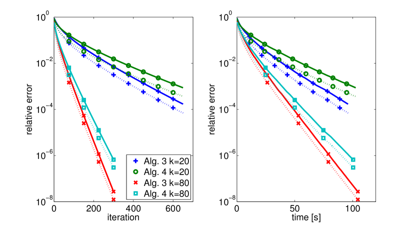
Fig. 1: Application of Algorithms 3 and 4 to (3.12) with $A\in\mathbb{R}^{2000\times 2000}$, $\mathop{\operator@font rank}\nolimits(A)=k$, for $k=20$ ($94.03\%$ missing entries), and $k=80$ ($76.48\%$ missing entries). Solid lines: relative errors (3.13) (full index set); dashed lines: relative errors (3.14) (sample index set).

Of course, Algorithms 3 and 4 served here only as examples and are naturally inferior to more sophisticated line-search methods, such as the nonlinear CG methods used in [50], which use gradient information from previous iterates.

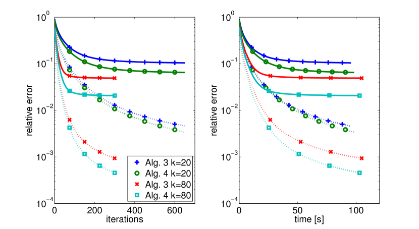
Fig. 2: Application of Algorithms 3 and 4 to (3.12) with $A\in\mathbb{R}^{2000\times 2000}$, $\mathop{\operator@font rank}\nolimits(A)=k/2$, for $k=20$ ($94.03\%$ missing entries), and $k=80$ ($76.48\%$ missing entries). Solid lines: relative errors (3.13) (full index set); dashed lines: relative errors (3.14) (sample index set).

4 Conclusion

We extended available results on convergence of descent iterations on manifolds via Łojasiewicz gradient inequality to gradient-related line-search methods on the real-algebraic variety $\mathcal{M}_{\leq k}$ of real $m\times n$ matrices of rank at most $k$, by explicitly taking the tangent cones at singular points into consideration. This made it possible to overcome some theoretical difficulties arising from the nonclosedness and unbounded curvature that one faces in the convergence analysis of Riemannian optimization methods on the smooth manifold $\mathcal{M}_{k}$ of rank-$k$ matrices. So far, the results are applicable for real-analytic cost functions.

There is growing interest in treating low-rank tensor problems by Riemannian optimization, e.g., tensor completion [25] or dynamical tensor approximation [22, 34, 48]. It would be important and interesting to extend the results to tensor varieties of bounded subspace ranks, e.g., bounded Tucker ranks, hierarchical Tucker ranks, or tensor train ranks [23, 16, 42]. As these varieties take the form of intersections of low-rank matrix varieties [48], the results in this paper can likely be generalized in this direction.

Appendix A Proof of Theorem 1

We can assume that $g^{-}_{n}>0$ for all $n$ since otherwise the sequence becomes stationary and there is nothing to prove. There will also be no loss of generality to assume that (A1) and (A2) hold for all $n$ and that $f(x^{*})=0$. Then $0\leq f(x^{*})\leq f_{n}$ for all $n$, and the Łojasiewicz gradient inequality at $x^{*}$ reads as

$$f(x)^{1-\theta}\leq\Lambda g^{-}(x)$$ (A.1)

whenever $\|x-x^{*}\|<\delta=\delta(x^{*})$. Let $\epsilon\in(0,\delta]$, and assume $\|x_{n}-x^{*}\|<\delta$. Then, by (A.1) and (A1),

$$\|x_{n}-x_{n+1}\|\leq\frac{\Lambda}{\sigma}f_{n}^{\theta-1}(f_{n}-f_{n+1}).$$

Using the fact that for $\varphi\in[f_{n+1},f_{n}]$ there holds $f_{n}^{\theta-1}\leq\varphi^{\theta-1}\leq f_{n+1}^{\theta-1}$, we can estimate

$$f_{n}^{\theta-1}(f_{n}-f_{n+1})\leq\int_{f_{n+1}}^{f_{n}}\varphi^{\theta-1}\,\mathrm{d}\varphi=\frac{1}{\theta}(f_{n}^{\theta}-f_{n+1}^{\theta})$$

and thus obtain

$$\|x_{n}-x_{n+1}\|\leq\frac{\Lambda}{\sigma\theta}(f_{n}^{\theta}-f_{n+1}^{\theta}).$$

More generally, let $\|x_{k}-x^{*}\|<\epsilon\leq\delta$ for $n\leq k<m$; we get by this argument that

$$\|x_{m}-x_{n}\|\leq\sum_{k=n}^{m}\|x_{k+1}-x_{k}\|\leq\sum_{k=n}^{m}\frac{\Lambda}{\sigma\theta}(f_{k}^{\theta}-f_{k+1}^{\theta})=\frac{\Lambda}{\sigma\theta}(f_{n}^{\theta}-f_{m}^{\theta})\leq\frac{\Lambda}{\sigma\theta}f_{n}^{\theta}.$$ (A.2)

Since $x^{*}$ is an accumulation point, we can pick $n$ so large that (recall that $f$ is continuous and $f(x^{*})=0$)

$$\|x_{n}-x^{*}\|<\frac{\epsilon}{2}\quad\text{and}\quad\frac{\Lambda}{\sigma\theta}f_{n}^{\theta}<\frac{\epsilon}{2}.$$

Then (A.2) inductively implies $\|x_{m}-x^{*}\|<\epsilon$ for all $m\geq n$. This proves that $x^{*}$ is the limit point of the sequence, and, by (A3), $g_{n}^{-}\to 0$.

To estimate the convergence rate, let $r_{n}=\sum_{k=n}^{\infty}\|x_{k+1}-x_{k}\|$. Then $\|x_{n}-x^{*}\|\leq r_{n}$, so it suffices to estimate the latter. By (A.2), (A.1), and (A3), there exists $n_{0}\geq 1$ such that for $n\geq n_{0}$ it holds that

$$r_{n}^{\frac{1-\theta}{\theta}}\leq\left(\frac{\Lambda}{\sigma\theta}\right)^{\frac{1-\theta}{\theta}}f_{n}^{1-\theta}\leq\left(\frac{\Lambda}{\sigma\theta}\right)^{\frac{1-\theta}{\theta}}\frac{\Lambda}{\kappa}\|x_{n+1}-x_{n}\|=\left(\frac{\Lambda}{\sigma\theta}\right)^{\frac{1-\theta}{\theta}}\frac{\Lambda}{\kappa}(r_{n}-r_{n+1}),$$

that is,

$$r_{n+1}\leq r_{n}-\nu r_{n}^{\frac{1-\theta}{\theta}}$$ (A.3)

with $\nu=(\frac{\Lambda}{\sigma\theta})^{\frac{\theta-1}{\theta}}\frac{\kappa}{\Lambda}$. Now, if $\theta=1/2$, we get from (A.3) that $\nu\in(0,1)$, and

$$r_{n}\leq r_{n_{0}}(1-\nu)^{n-n_{0}}\left(e^{\ln(1-\nu)}\right)^{n}$$

for $n\geq n_{0}$. The case $0<\theta<1/2$ is more delicate. We follow Levitt [30]: put $p=\frac{\theta}{1-2\theta}$, $C\geq\max((\frac{\nu}{p})^{-p},r_{n_{0}}n_{0}^{-p})$, and $s_{n}=Cn^{-p}$; then $s_{n_{0}}\geq r_{n_{0}}$, and

$$s_{n+1}=s_{n}(1+n^{-1})^{-p}\geq s_{n}(1-pn^{-1})=s_{n}-\frac{p}{C^{1/p}}s_{n}^{\frac{p+1}{p}}\geq s_{n}-\nu s_{n}^{\frac{p+1}{p}}=s_{n}-\nu s_{n}^{\frac{1-\theta}{\theta}}$$

(the first inequality holding by convexity of $x^{-p}$). Using induction, it now follows from (A.3) that $r_{n}\leq s_{n}$ for all $n\geq n_{0}$, which finishes the proof.

References

- [1] P.-A. Absil, R. Mahony, and B. Andrews, Convergence of the iterates of descent methods for analytic cost functions, SIAM J. Optim., 16 (2005), pp. 531–547.
- [2] P.-A. Absil, R. Mahony, and R. Sepulchre, Optimization Algorithms on Matrix Manifolds, Princeton University Press, Princeton, NJ, 2008.
- [3] P.-A. Absil and J. Malick, Projection-like retractions on matrix manifolds, SIAM J. Optim., 22 (2012), pp. 135–158.
- [4] H. Attouch and J. Bolte, On the convergence of the proximal algorithm for nonsmooth functions involving analytic features, Math. Program., 116 (2009), pp. 5–16.
- [5] H. Attouch, J. Bolte, P. Redont, and A. Soubeyran, Proximal alternating minimization and projection methods for nonconvex problems: An approach based on the Kurdyka-Łojasiewicz inequality, Math. Oper. Res., 35 (2010), pp. 438–457.
- [6] H. Attouch, J. Bolte, and B.F. Svaiter, Convergence of descent methods for semi-algebraic and tame problems: Proximal algorithms, forward-backward splitting, and regularized Gauss-Seidel methods, Math. Program., 137 (2013), pp. 91–129.
- [7] J. Bolte, A. Daniilidis, and A. Lewis, The Łojasiewicz inequality for nonsmooth subanalytic functions with applications to subgradient dynamical systems, SIAM J. Optim., 17 (2007), pp. 1205–1223.
- [8] J. Bolte, A. Daniilidis, A. Lewis, and M. Shiota, Clarke subgradients of stratifiable functions, SIAM J. Optim., 18 (2007), pp. 556–572.
- [9] J. Bolte, A. Daniilidis, O. Ley, and L. Mazet, Characterizations of Łojasiewicz inequalities: Subgradient flows, talweg, convexity, Trans. Amer. Math. Soc., 362 (2010), pp. 3319–3363.
- [10] A. Bunse-Gerstner, R. Byers, V. Mehrmann, and N.K. Nichols, Numerical computation of an analytic singular value decomposition of a matrix valued function, Numer. Math., 60 (1991), pp. 1–39.
- [11] S. Burer and R.D.C. Monteiro, A nonlinear programming algorithm for solving semidefinite programs via low-rank factorization, Math. Program., 95 (2003), pp. 329–357.
- [12] E. Cancès, V. Ehrlacher, and T. Lelièvre, Greedy algorithms for high-dimensional eigenvalue problems, Constr. Approx., 40 (2014), pp. 387–423.
- [13] T.P. Cason, P.-A. Absil, and P. Van Dooren, Iterative methods for low rank approximation of graph similarity matrices, Linear Algebra Appl., 438 (2013), pp. 1863–1882.
- [14] J. Dieudonné, Treatise on Analysis. Vol. III, Academic Press, New York, London, 1972.
- [15] M. Guignard, Generalized Kuhn–Tucker conditions for mathematical programming problems in a Banach space, SIAM J. Control, 7 (1969), pp. 232–241.
- [16] W. Hackbusch and S. Kühn, A new scheme for the tensor representation, J. Fourier Anal. Appl., 15 (2009), pp. 706–722.
- [17] A. Haraux and M.A. Jendoubi, The Łojasiewicz gradient inequality in the infinite-dimensional Hilbert space framework, J. Funct. Anal., 260 (2011), pp. 2826–2842.
- [18] U. Helmke and M.A. Shayman, Critical points of matrix least squares distance functions, Linear Algebra Appl., 215 (1995), pp. 1–19.
- [19] S.-Z. Huang, Gradient Inequalities. With Applications to Asymptotic Behavior and Stability of Gradient-like Systems, American Mathematical Society, Providence, RI, 2006.
- [20] M. Journée, F. Bach, P.-A. Absil, and R. Sepulchre, Low-rank optimization on the cone of positive semidefinite matrices, SIAM J. Optim., 20 (2010), pp. 2327–2351.
- [21] O. Koch and C. Lubich, Dynamical low-rank approximation, SIAM J. Matrix Anal. Appl., 29 (2007), pp. 434–454.
- [22] , Dynamical tensor approximation, SIAM J. Matrix Anal. Appl., 31 (2010), pp. 2360–2375.
- [23] T.G. Kolda and B.W. Bader, Tensor decompositions and applications, SIAM Rev., 51 (2009), pp. 455–500.
- [24] S.G. Krantz and H.R. Parks, A Primer of Real Analytic Functions, Birkhäuser Boston Boston, 2nd ed., 2002.
- [25] D. Kressner, M. Steinlechner, and B. Vandereycken, Low-rank tensor completion by Riemannian optimization, BIT, 54 (2014), pp. 447–468.
- [26] K. Kurdyka, On gradients of functions definable in o-minimal structures, Ann. Inst. Fourier (Grenoble), 48 (1998), pp. 769–783.
- [27] C. Lageman, Konvergenz reell-analytischer gradientenähnlicher Systeme, diploma thesis, Universität Würzburg, Würzburg, Germany, 2002. In German.
- [28] , Convergence of Gradient-like Dynamical Systems and Optimization Algorithms, PhD thesis, Universität Würzburg, Würzburg, Germany, 2007.
- [29] , Pointwise convergence of gradient-like systems, Math. Nachr., 280 (2007), pp. 1543–1558.
- [30] A. Levitt, Convergence of gradient-based algorithms for the Hartree-Fock equations, ESAIM Math. Model. Numer. Anal., 46 (2012), pp. 1321–1336.
- [31] Z. Li, A. Uschmajew, and S. Zhang, On convergence of the maximum block improvement method, SIAM J. Optim., 25 (2015), pp. 210–233.
- [32] S. Łojasiewicz, Ensemble semi-analytique. Note des cours, Institut des Hautes Etudes Scientifique, 1965.
- [33] C. Lubich and I.V. Oseledets, A projector-splitting integrator for dynamical low-rank approximation, BIT, 54 (2014), pp. 171–188.
- [34] C. Lubich, T. Rohwedder, R. Schneider, and B. Vandereycken, Dynamical approximation by hierarchical Tucker and tensor-train tensors, SIAM J. Matrix Anal. Appl., 34 (2013), pp. 470–494.
- [35] D.R. Luke, Prox-regularity of rank constraints sets and implications for algorithms, J. Math. Imaging Vision, 47 (2013), pp. 231–238.
- [36] B. Merlet and T.N. Nguyen, Convergence to equilibrium for discretizations of gradient-like flows on Riemannian manifolds, Differential Integral Equations, 26 (2013), pp. 571–602.
- [37] B. Mishra, G. Meyer, F. Bach, and R. Sepulchre, Low-rank optimization with trace norm penalty, SIAM J. Optim., 23 (2013), pp. 2124–2149.
- [38] B. Mishra, G. Meyer, S. Bonnabel, and R. Sepulchre, Fixed-rank matrix factorizations and Riemannian low-rank optimization, Comput. Statist., 29 (2014), pp. 591–621.
- [39] J. Nocedal and S.J. Wright, Numerical Optimization, Springer, New York, 2006.
- [40] D. Noll, Convergence of non-smooth descent methods using the Kurdyka-Łojasiewicz inequality, J. Optim. Theory Appl., 160 (2014), pp. 553–572.
- [41] A. Nonnenmacher and C. Lubich, Dynamical low-rank approximation: Applications and numerical experiments, Math. Comput. Simulation, 79 (2008), pp. 1346–1357.
- [42] I.V. Oseledets, Tensor-train decomposition, SIAM J. Sci. Comput., 33 (2011), pp. 2295–2317.
- [43] D.B. O’Shea and L.C. Wilson, Limits of tangent spaces to real surfaces, Amer. J. Math., 126 (2004), pp. 951–980.
- [44] R.T. Rockafellar and R.J.-B. Wets, Variational Analysis, Springer-Verlag, Berlin, 1998.
- [45] U. Shalit, D. Weinshall, and G. Chechik, Online learning in the embedded manifold of low-rank matrices, J. Mach. Learn. Res., 13 (2012), pp. 429–458.
- [46] M. Shub, Some remarks on dynamical systems and numerical analysis, in Dynamical Systems and Partial Differential Equations (Caracas, 1984), Univ. Simon Bolivar, Caracas, 1986, pp. 69–91.
- [47] M. Tan, I. W. Tsang, L. Wang, B. Vandereycken, and S. J. Pan, Riemannian pursuit for big matrix recovery, in Proceedings of the 31st International Conference on Machine Learning (ICML), vol. 32 of JMLR Workshop and Conference Proceedings, 2014, pp. 1539–1547.
- [48] A. Uschmajew and B. Vandereycken, The geometry of algorithms using hierarchical tensors, Linear Algebra Appl., 439 (2013), pp. 133–166.
- [49] , Line-search methods and rank increase on low-rank matrix varieties, in Proceedings of the 2014 International Symposium on Nonlinear Theory and its Applications (NOLTA2014), 2014, pp. 52–55.
- [50] B. Vandereycken, Low-rank matrix completion by Riemannian optimization, SIAM J. Optim., 23 (2013), pp. 1214–1236.
- [51] B. Vandereycken and S. Vandewalle, A Riemannian optimization approach for computing low-rank solutions of Lyapunov equations, SIAM J. Matrix Anal. Appl., 31 (2010), pp. 2553–2579.
- [52] Y. Xu and W. Yin, A block coordinate descent method for regularized multiconvex optimization with applications to nonnegative tensor factorization and completion, SIAM J. Imaging Sci., 6 (2013), pp. 1758–1789.