Channel Diversity needed for Vector Space Interference Alignment

Abstract

We consider vector space interference alignment strategies over the $K$-user interference channel and derive an upper bound on the achievable degrees of freedom as a function of the channel diversity $L$, where the channel diversity is modeled by $L$ real-valued parallel channels with coefficients drawn from a non-degenerate joint distribution. The seminal work of Cadambe and Jafar shows that when $L$ is unbounded, vector space interference alignment can achieve $1/2$ degrees of freedom per user independent of the number of users $K$. However wireless channels have limited diversity in practice, dictated by their coherence time and bandwidth, and an important question is the number of degrees of freedom achievable at finite $L$. When $K=3$ and if $L$ is finite, Bresler et al show that the number of degrees of freedom achievable with vector space interference alignment is bounded away from $1/2$, and the gap decreases inversely proportional to $L$. In this paper, we show that when $K\geq 4$, the gap is significantly larger. In particular, the gap to the optimal $1/2$ degrees of freedom per user can decrease at most like $1/\sqrt{L}$, and when $L$ is smaller than the order of $2^{(K-2)(K-3)}$, it decays at most like $1/\sqrt[4]{L}$.

I Introduction

Interference is the central phenomenon severely limiting the performance of most wireless systems. Over the recent years, interference alignment has emerged as a promising tool to mitigate interference [1, 2]. The main idea is to design transmit signals of different users in such a way that, upon arriving at the unintended receivers, they overlap with each other and the resulting interference is perceived as much less than the sum of the individual interferences. Surprisingly, the work [2] of Cadambe and Jafar has shown that this approach can lead to $K/2$ sum degrees of freedom over the time or frequency-varying $K$-user interference channel, while traditional approaches such as treating interference as noise or orthogonalizing transmissions can provide only one degree of freedom. This roughly implies that at high-SNR, each user can communicate as if it has half the resources of the channel for its exclusive use, regardless of the total number of users.

However, one of the main caveats of the $K/2$ degrees of freedom result in [2] is that it requires unbounded time or frequency variation of the channel. More precisely, in order to achieve $K/2$ degrees of freedom, the transmitters have to code over the order of $K^{K^{2}}$ independent realizations of the channel (or equivalently $K^{K^{2}}$ parallel channels). (This scaling is slightly improved to $2^{K^{2}}$ by Özgür and Tse [3].) In practice, wireless channels have finite channel diversity dictated by their coherence time and bandwidth, and the requirement $K^{K^{2}}$ is prohibitive even for small values of $K$. Whether this exponential requirement for channel diversity is fundamental or not to vector space interference alignment strategies, of which the scheme in [2] is one specific example, is an important question in determining the real potential of interference alignment in practical wireless systems.

Despite significant research interest in interference alignment over the recent years (see [4] for an overview), there is limited understanding regarding this question, and more generally, regarding how the available channel diversity impacts the ability to align interference. The problem is understood only in the case when $K=3$. In this case, Bresler and Tse [5] characterize the exact relation between the channel diversity $L$, modeled by the number of independent channel realizations over time or frequency, and the total number of degrees of freedom achievable using vector space alignment. (Their result subsumes an earlier result by Cadambe, Jafar and Wang [6] which corresponds to the special case $L=2$.) They show that the achievable sum degrees of freedom in the $3$-user interference channel are given by

$$\mathrm{DoF}=\frac{3}{2}\left(1-\frac{1}{4L-2\lfloor L/2\rfloor-1}\right).$$ (1)

We can observe that when $L\rightarrow\infty$, $3/2$ degrees of freedom are achievable as expected, and for finite values of $L$ the formula precisely characterizes how $\mathrm{DoF}$ approaches $3/2$ as a function of $L$. To our knowledge, nothing is known regarding the relation between channel diversity and achievable degrees of freedom for interference channels with more than $3$-users; apart from the trivial conclusion that when $L=1$, vector interference alignment can achieve only one degree of freedom and the result of [2] which shows that when $L\rightarrow\infty$, $K/2$ degrees of freedom are achievable.

In this paper, which is an extended and more complete version of [7], we make progress in this direction by first showing that for $K\geq 4$,

$$\mathrm{DoF}\leq\frac{K}{2}\left(1-\frac{1}{11\sqrt{L}}\right).$$

This result shows that the degrees of freedom per user approach $1/2$ at a much slower speed when $K\geq 4$ when compared to $K=3$: the gap decreases at most like $1/\sqrt{L}$ as opposed to $1/L$. Next, we further improve our result to

$$\mathrm{DoF}\leq\frac{K}{2}\left(1-C\min\left\{\frac{1}{\sqrt[4]{L}},\frac{2^{\left(K-2\right)\left(K-3\right)/4}}{\sqrt{L}}\right\}\right),$$

where $C>0$ is a constant. In the regime when $L$ is smaller than the order of $2^{\left(K-2\right)\left(K-3\right)}$, i.e., when the first term of the minimum is smaller than the second, this implies that the gap to the optimal $1/2$ degrees of freedom per user decreases at most like $1/\sqrt[4]{L}$. As a result, when $K$ grows, either we need an exponential channel diversity $L>2^{\left(K-2\right)\left(K-3\right)}$, or the gap to the optimal 1/2 degrees of freedom per user decreases at most like $1/\sqrt[4]{L}$.

A closer look at the scheme in [2] reveals that the following degrees of freedom are achievable over the $K$-user interference channel for $L$ large enough.

$$\mathrm{DoF}\geq\frac{K}{2}\left(1-\frac{CN}{\sqrt[N]{L/2}}\right),$$ (2)

where $N=(K-1)(K-2)-1$ and $C>0$ is a constant. When $K=3$, we have $N=1$ and this matches the scaling in (1). When $K=4$, we have $N=5$ which implies that gap to the optimal degrees of freedom decreases like $1/\sqrt[5]{L}$ in (2), while our upper bound only implies that the gap can not decrease faster than $1/\sqrt{L}$ ($1/\sqrt[4]{L}$ when $L$ is smaller than the order of $2^{\left(K-2\right)\left(K-3\right)}$). The difference between the scaling of our upper bound and the achievability in (2) becomes even larger as $K$ increases.

While the remaining gap between the lower bound (2) and the upper bounds we derive is still quite large, one of the main contributions of this paper is to build a mathematical framework (tools and notions) for studying the alignment problem when $K\geq 4$. Note that the case $K\geq 4$ is significantly more complex than the case $K=3$, in which case it is possible to explicitly keep track of how intertwined the users’ signaling strategies are due to alignment. The exact characterization in (1) is indeed based on such explicit tracking of users’ signaling spaces. For $K\geq 4$, there is significantly more freedom in choosing user’s signaling spaces and it is not possible to keep track of the intertwining between them. Without such explicit tracking, we provide a framework that allows to capture the tradeoff between the two requirements of aligning interference at the unintended receivers and that of keeping the desired signal space distinct from interference at the intended receivers. We believe this framework can be further developed to prove tighter results in the future.

I-A Related Work

A related problem has been considered in a recent paper [8], which restricts each transmitter to send a single beam (the signaling space of each transmitter has dimension one) and asks how many transmitter-receiver pairs can be accommodated when the channel diversity is finite. Their approach combines counting arguments with algebraic tools to determine the feasibility of a hybrid system of equations and inequalities. In contrast here we do not restrict the dimension of the signaling space at each transmitter. Indeed, [2] shows that the benefits of the interference alignment are asymptotic in nature and can be realized by increasing the dimension of the signaling space at the transmitters, which leads to more freedom in the choice of the signaling spaces. This, however, also makes the problem of characterizing the achievable degrees of freedom more difficult and in particular one can not rely on explicit counting arguments as in [8].

Another related line of research [9, 10, 11, 12] (see also [4] and the references therein) looks at the relation between the spatial diversity available in a MIMO interference channel and the degrees of freedom achievable with vector interference alignment strategies. Here each user is equipped with multiple antennas and signals are aligned over the spatial dimension with no time/frequency diversity in the channel. The impact of the spatial diversity (number of transmit and receive antennas) on the achievable degrees of freedom with vector interference alignment strategies is much better understood. For example, [13] shows that in the symmetric case where each node is equipped with $N$ antennas, the maximum number of $\mathrm{DoF}$ achievable with vector space alignment strategies is given by

$$\mathrm{DoF}=K\left\lfloor\frac{2N}{K+1}\right\rfloor\leq 2N\frac{K}{K+1}.$$

In sharp contrast to the $K/2$ degrees of freedom achievable with time/frequency diversity, this result implies that the $\mathrm{DoF}$ gain from aligning interference over the spatial dimension is limited by a factor of $2$ when compared to the $\mathrm{DoF}$ achieved with simple orthogonalization of users’ transmissions. This implies that the gain from spatial interference alignment is very limited when compared to the potential gain from aligning interference over time/frequency varying channels. Therefore, we believe understanding the feasibility of interference alignment over time/frequency varying channels with limited diversity is the key to assessing the real potential of interference alignment strategies in practical systems.

II Problem Formulation

II-A Notation

For a vector $\mathbf{v}\in\mathbb{R}^{L}$, we write $\left\|\mathbf{v}\right\|_{0}$ for the number of nonzero entries of $\mathbf{v}$. For $\mathbf{H}\in\mathbb{R}^{L\times L}$ and subspace $V\subseteq\mathbb{R}^{L}$, we write $\mathbf{H}V$ for the subspace $\{\mathbf{H}\mathbf{v}\,:\,\mathbf{v}\in V\}$. For subspaces $V_{1},V_{2},...,V_{n}\subseteq\mathbb{R}^{L}$, we write $V_{1}+V_{2}=\mathrm{span}\left(V_{1}\cup V_{2}\right)$, and $\sum_{i=1}^{n}V_{i}=V_{1}+\cdots+V_{n}$. We write $\left\langle\mathbf{v}_{1},...,\mathbf{v}_{n}\right\rangle=\mathrm{span}\left\{\mathbf{v}_{1},...,\mathbf{v}_{n}\right\}$. For a subset $S\subseteq\left\{1,...,L\right\}$, $\mathbb{R}^{S}=\{\mathbf{v}\in\mathbb{R}^{L}:\,\mathbf{v}_{i}=0\;\text{for all}\;i\notin S\}$. The $L\times L$ identity matrix is denoted by $\mathbf{I}_{L}$ ($L$ may be omitted when the dimension is clear in the context). For a vector $\mathbf{v}\in\mathbb{R}^{L}$, we write $\mathrm{diag}(\mathbf{v})\in\mathbb{R}^{L\times L}$ for the diagonal matrix formed by the entries of $\mathbf{v}$. For $\mathbf{X}\in\mathbb{R}^{L\times L}$, we write $\mathrm{diag}(\mathbf{X})\in\mathbb{R}^{L}$ for the vector formed by the diagonal entries of $\mathbf{X}$.

II-B Channel Model

Consider the fully-connected $K$-user Gaussian interference channel, where receiver $i$ wants to obtain a message from transmitter $i$ for $1\leq i\leq K$, but the signal received is superimposed by interferences from transmitters $j\neq i$. The input-output relationship is given by

$$\mathbf{y}_{i}=\sum_{j=1}^{K}\mathbf{H}_{ij}\mathbf{x}_{j}+\mathbf{z}_{i},$$ (3)

where $\mathbf{x}_{i}\in\mathbb{R}^{L}$ is the transmitted signal of transmitter $i$ over $L$ channel uses; $\mathbf{y}_{i}\in\mathbb{R}^{L}$ is the received signal of receiver $i$; $\mathbf{z}_{i}\sim\mathcal{N}\left(0,\mathbf{I}\right)$ is an additive white Gaussian noise; and $\mathbf{H}_{ij}\in\mathbb{R}^{L\times L}$ is a diagonal matrix containing the channel coefficients from Transmitter $j$ to Receiver $i$ over the $L$ channel uses,

$$\mathbf{H}_{ij}=\left[\begin{array}[]{ccc}h_{ij}^{(1)}\\ &\ddots\\ &&h_{ij}^{(L)}\end{array}\right].$$

We assume the entries of $\mathbf{H}_{ij}$ are chosen i.i.d. from a continuous distribution, or more generally, the joint distribution of $\left\{(\mathbf{H}_{ij})_{\ell\ell}\right\}_{i,j=1,...,K,\,\ell=1,...,L}$ has a density in the $LK^{2}$-dimensional space. This channel model corresponds to $L$ uses of a fast fading interference channel where we get a different realization of the channel at each use.

The integer $L$ is called the diversity of the channel. In the above model it is related to the blocklength of communication, and more precisely, it is the number of coherence periods over which we code. For the block fading case where each coherence period is of duration $T$, $\mathbf{H}_{ij}$ are the diagonal matrices formed by $h_{ij}^{(1)},\ldots,h_{ij}^{(1)},h_{ij}^{(2)},\ldots,h_{ij}^{(2)},h_{ij}^{(3)},\ldots,h_{ij}^{(L)}$, where each $h_{ij}^{(l)}$ is repeated $T$ times, i.e., $\mathbf{H}_{ij}=\mathrm{diag}\left[h_{ij}^{(1)},...,h_{ij}^{(L)}\right]\otimes\mathbf{I}_{T}\in\mathbb{R}^{TL\times TL}$, where $\otimes$ denotes the Kronecker product. In this paper, we first consider the fast fading case ($T=1$) and then extend our results to the block fading case.

II-C Vector Interference Alignment Strategies and Degrees of Freedom

In this paper we focus on vector space schemes, which we specify next. Suppose transmitter $i$ wishes to transmit $\widehat{\mathbf{x}}_{i}\in\mathbb{R}^{D}$ containing $D$ data symbols. It applies a precoding matrix $\mathbf{V}_{i}\in\mathbb{R}^{L\times D}$ and transmits $\mathbf{x}_{i}=\mathbf{V}_{i}\widehat{\mathbf{x}}_{i}$. Let $V_{i}\subseteq\mathbb{R}^{L}$ be the column span of $\mathbf{V}_{i}$. Receiver $i$ decodes $\widehat{\mathbf{x}}_{i}$ by zero-forcing interference, i.e., projecting its received signal on the orthogonal complement of the space spanned by the interference. At high SNR, it can decode the $D$ data symbols if the signal subspace $\mathbf{H}_{ii}V_{i}$ intersects the interference subspace only at 0, i.e.,

$$\mathbf{H}_{ii}V_{i}\cap\biggl{(}\sum_{j\neq i}\mathbf{H}_{ij}V_{j}\biggr{)}=\left\{0\right\}.$$

We call this the decoding condition at receiver $i$. The maximum total degrees of freedom achievable by this strategy is given by

$$\mathrm{DoF}=\max_{\left\{V_{i}\right\}\text{ satisfies decoding condition }\forall i}KD/L.$$

It is easy to observe that this corresponds to the classical degrees of freedom definition for the interference channel: In particular assume that the transmitted signals $\mathbf{x}_{i}\in\mathbb{R}^{L}$ in (3) are subject to an average power constraint $LP$, i.e. average power $P$ per channel use. The total degrees of freedom achieved by the vector interference alignment strategy can be equivalently defined as

$$\mathrm{DoF}=\lim_{P\to\infty}\frac{1}{L}\frac{R(P)}{\log P}$$

where $R(P)$ denotes the rate achieved by this strategy under a per user power constraint $P$.

If we wish to have $\mathrm{DoF}\geq\left(1-\epsilon\right)K/2$, then $D\geq\left(1-\epsilon\right)L/2$. Given that the signalling subspaces $V_{i}$ have to satisy the decoding condition at each receiver, the goal of this paper is to give a lower bound on the channel diversity $L$ in terms of the gap $\epsilon$. This translates to an upper bound on the achievable degrees of freedom with any given channel diversity $L$.

In the block fading case, the signal space is $V_{i}\subseteq\mathbb{R}^{TL}$ instead of $V_{i}\subseteq\mathbb{R}^{L}$, and therefore the definition of maximum total degrees of freedom is modified as

$$\mathrm{DoF}=\max_{\left\{V_{i}\right\}\text{ satisfies decoding condition }\forall i}\frac{KD}{TL}.$$

III Main Result

The following theorem is the main result of this paper.

Theorem 1.

In the fast fading case ($T=1$), when $K\geq 4$, with probability $1$, the maximum sum degrees of freedom achievable with vector space interference alignment strategies is bounded by

$$\mathrm{DoF}\leq\frac{K}{2}\left(1-\frac{1}{11\sqrt{L}}\right).$$

The theorem can be extended to block fading, at the expense of a larger constant.

Theorem 2.

In the block fading case for any value of $T\geq 1$, when $K\geq 4$, with probability $1$, the maximum sum degrees of freedom achievable with vector space interference alignment strategies is bounded by

$$\mathrm{DoF}\leq\frac{K}{2}\left(1-\frac{1}{20\sqrt{L}}\right).$$

The result can be improved for large $L$ and $K$ to the following result.

Theorem 3.

In the fast fading or block fading case for any value of $T\geq 1$, when $K\geq 4$, with probability $1$, the maximum total degrees of freedom is bounded by

$$\mathrm{DoF}\leq\frac{K}{2}\left(1-2^{-17}\min\left\{\frac{1}{\sqrt[4]{L}},\frac{2^{\left(K-2\right)\left(K-3\right)/4}}{\sqrt{L}}\right\}\right).$$

Although the constant in this theorem is quite small, we believe the theorem and its proof are important in illustrating how the notions and the tools we develop to tackle this problem (such as extension and contraction of a subspace defined in the next section) can be further developed in nontrivial ways to obtain tighter results.

The rest of the paper is devoted to the proof of the theorems. In Section IV, we define and develop three notions: the alignment width of a subspace, the sparsity of a subspace, and the linear independence condition for a set of diagonal matrices which allow us to convert the problem of interest to a pure linear algebra problem. In Section V-A, we provide the intuition for our proof under a simplifying assumption. The proof of our main result for fast fading (Theorem 1) is given in Section V-B, and for block fading (Theorem 2) in Section VI. Theorem 3 is proved in Section VII.

IV A Linear Algebra problem

Below, we focus on the case $K\geq 4$. We assume that the diagonal entries of $\mathbf{H}_{ij}$ are nonzero, which holds with probability 1.

IV-A Alignment Width

Definition 1 (Extension and contraction operators).

Let $V\subseteq\mathbb{R}^{L}$ be a subspace, and $\mathbf{T}\in\mathbb{R}^{L\times L}$ be a diagonal matrix with non-zero diagonal entries. Define the extension operator $\mathrm{e}_{\mathbf{T}}$ and the contraction operator $\mathrm{c}_{\mathbf{T}}$ by

$$\mathrm{e}_{\mathbf{T}}V = V+\mathbf{T}V,$$

$$\mathrm{e}_{\mathbf{T}}^{n}V = V+\mathbf{T}V+\cdots+\mathbf{T}^{n}V,$$

$$\mathrm{c}_{\mathbf{T}}V = V\cap\mathbf{T}V,$$

$$\mathrm{c}_{\mathbf{T}}^{n}V = V\cap\mathbf{T}V\cap\cdots\cap\mathbf{T}^{n}V.$$

Definition 2 (Alignment width).

We define the alignment width of a subspace $V$ under a diagonal matrix $\mathbf{T}$ by

$$\Delta_{\mathbf{T}}V = \dim\left(\mathrm{e}_{\mathbf{T}}V\right)-\dim V$$

$$= \dim V-\dim\left(\mathrm{c}_{\mathbf{T}}V\right),$$

The equality is due to

$$\dim(V+W) =\dim(V)+\dim(W)-\dim(V\cap W)$$ (4)

for subspaces $V,W$. This equality will be used extensively throughout the paper. Intuitively, the alignment width is a measure of the difference between $V$ and its rotated version $\mathbf{T}V$; it is the dimension of the subspace which jumps out of the original subspace after the linear transformation by $\mathbf{T}$. Equivalently, according to the second equivalent definition it can be thought of as the dimension of the part of $V$ that does not align with $\mathbf{T}V$. This is illustrated in Figure 1.

There are several properties of extension and contraction operators that follow directly from their definitions and will be used repeatedly throughout the paper. Extensions along different matrices commute with each other, and so do contractions, i.e.,

$$\mathrm{e}_{\mathbf{T}_{1}}\mathrm{e}_{\mathbf{T}_{2}}V =\mathrm{e}_{\mathbf{T}_{2}}\mathrm{e}_{\mathbf{T}_{1}}V,$$

$$\mathrm{c}_{\mathbf{T}_{1}}\mathrm{c}_{\mathbf{T}_{2}}V =\mathrm{c}_{\mathbf{T}_{2}}\mathrm{c}_{\mathbf{T}_{1}}V.$$

However, extension and contraction do not commute with each other. Instead the following holds

$$\mathrm{e}_{\mathbf{T}_{1}}\mathrm{c}_{\mathbf{T}_{2}}V \subseteq\mathrm{c}_{\mathbf{T}_{2}}\mathrm{e}_{\mathbf{T}_{1}}V.$$ (5)

Moreover,

$$\mathrm{e}_{\mathbf{T}}\mathrm{c}_{\mathbf{T}^{-1}}V \subseteq V\subseteq\mathrm{c}_{\mathbf{T}^{-1}}\mathrm{e}_{\mathbf{T}}V.$$ (6)

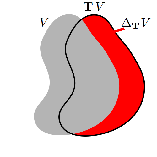
Figure 1: Illustration of alignment width of $V$ under $\mathbf{T}$. Multiplication by $\mathbf{T}$ is represented by a shift to the right.

Now, define

$$\mathbf{T}_{ijk}=\mathbf{H}_{1i}^{-1}\mathbf{H}_{1k}\mathbf{H}_{jk}^{-1}\mathbf{H}_{ji}.$$

Since the matrices $\mathbf{H}_{ij}$ are drawn from a continuous distribution, the matrix $\mathbf{T}_{ijk}$ is almost surely defined and invertible, and hence we assume this throughout the paper. In the following lemma, we show that if the subspaces $V_{i}$ satisfy the decoding condition, then they have to “align” with these diagonal matrices $\mathbf{T}_{ijk}$ in the sense that $V_{i}$ has a large intersection with $\mathbf{T}_{ijk}V_{i}$, i.e., $\Delta_{\mathbf{T}_{ijk}}V_{i}$ is small. The lemma builds on the observation that if two signal subspaces $V_{i}$ and $V_{k}$ have nearly the same projections at two receivers where they consitute interference say Receiver $1$ and Receiver $j$, then $\mathbf{H}_{1i}V_{i}\approx\mathbf{H}_{1k}V_{k}$ and $\mathbf{H}_{ji}V_{i}\approx\mathbf{H}_{jk}V_{k}$. Hence

$$\mathbf{H}_{1i}^{-1}\mathbf{H}_{1k}\mathbf{H}_{jk}^{-1}\mathbf{H}_{ji}V_{i}\approx\mathbf{H}_{1i}^{-1}\mathbf{H}_{1k}V_{j}\approx V_{i}.$$

Lemma 1 (Width requirement for decoding).

If $D=\left(1-\epsilon\right)L/2$ and $V_{i},\,i=1,\dots,K$ satisfy the decoding condition at all the receivers, then $\Delta_{\mathbf{T}_{ijk}}V_{i}\leq 2\epsilon L$ for all distinct $i,j,k\neq 1$.

Proof:

Due to the decoding condition at receiver $1$, for any distinct $i,k\neq 1$ we have

$$\dim\left(\mathbf{H}_{1i}V_{i}\!+\!\mathbf{H}_{1k}V_{k}\right)=\dim\left(V_{i}\!+\!\mathbf{H}_{1i}^{-1}\mathbf{H}_{1k}V_{k}\right)\leq\left(1+\epsilon\right)L/2.$$

Due to the decoding condition at receiver $j\neq 1$, we have

$$\dim\left(\mathbf{H}_{ji}V_{i}\!+\!\mathbf{H}_{jk}V_{k}\right)\!=\!\dim\left(\mathbf{T}_{ijk}V_{i}\!+\!\mathbf{H}_{1i}^{-1}\mathbf{H}_{1k}V_{k}\right)\!\leq\!\left(1+\epsilon\right)L/2.$$

for any distinct $i,j,k$. Let $\widehat{V}_{k}=\mathbf{H}_{1i}^{-1}\mathbf{H}_{1k}V_{k}$. Then by (4),

$$\dim\left(V_{i}\cap\widehat{V}_{k}\right)$$

$$=\dim\left(V_{i}\right)+\dim\left(\widehat{V}_{k}\right)-\dim\left(V_{i}+\widehat{V}_{k}\right)$$

$$\geq 2D-\left(1+\epsilon\right)L/2,$$

and similarly we have $\dim\left(\mathbf{T}_{ijk}V_{i}\cap\widehat{V}_{k}\right)\geq 2D-\left(1+\epsilon\right)L/2$. Hence again using(4), we have

$$\dim\left(V_{i}\cap\mathbf{T}_{ijk}V_{i}\right)$$

$$\geq \dim\left(V_{i}\cap\mathbf{T}_{ijk}V_{i}\cap\widehat{V}_{k}\right)$$

$$= \dim\left((V_{i}\cap\widehat{V}_{k})\cap(\mathbf{T}_{ijk}V_{i}\cap\widehat{V}_{k})\right)$$

$$= \dim\left(V_{i}\cap\widehat{V}_{k}\right)+\dim\left(\mathbf{T}_{ijk}V_{i}\cap\widehat{V}_{k}\right)$$

$$\;-\dim\left((V_{i}\cap\widehat{V}_{k})+(\mathbf{T}_{ijk}V_{i}\cap\widehat{V}_{k})\right)$$

$$\geq \dim\left(V_{i}\cap\widehat{V}_{k}\right)+\dim\left(\mathbf{T}_{ijk}V_{i}\cap\widehat{V}_{k}\right)-\dim(\widehat{V}_{k})$$

$$\geq 3D-\left(1+\epsilon\right)L$$

and

$$\Delta_{\mathbf{T}_{ijk}}V_{i} = D-\dim\left(V_{i}\cap\mathbf{T}_{ijk}V_{i}\right)$$

$$\leq D-\left(3D-\left(1+\epsilon\right)L\right)$$

$$= 2\epsilon L,$$

which completes the proof of the lemma. ∎

IV-B Sparsity of Subspaces

In this section, we define the sparsity of a subspace and show that if $V_{i}$ satisfy the decoding condition then they cannot have low sparsity.

Definition 3.

($N$-sparsity) We define the $N$-sparsity of a subspace $V\subseteq\mathbb{R}^{L}$ as

$$\mathrm{sp}_{N}\left(V\right)\!\! \!\!=\!\! \!\!\min\left\{\left|S\right|\,:\,S\subseteq\left\{1,...,L\right\},\,\dim\left(V\cap\mathbb{R}^{S}\right)\geq N\right\}$$

$$\!\!=\!\! \!\!\min\left\{\max_{\mathbf{v}\in W}\left\|\mathbf{v}\right\|_{0}\,:\,W\subseteq V,\,\dim\left(W\right)\geq N\right\}.$$

When $N>\dim V$, let $\mathrm{sp}_{N}\left(V\right)=\infty$.

The $N$-sparsity of a subspace $V$ quantifies the sparsity of its sparsest $N$-dimensional subspace. Consider the first definition: if $\mathrm{sp}_{N}(V)=d$, then there exists an $N$-dimensional subspace of $V$, call it $W$, which is fully contained in $\mathbb{R}^{S}$ for some $S\subseteq\left\{1,...,L\right\}$ such that $|S|=d$, i.e., $W$ is composed of vectors with all entries other than those in $S$ equal to zero. (This immediately implies that $\mathrm{sp}_{N}(V)\geq N$.) Hence, $\max_{\mathbf{v}\in W}\left\|\mathbf{v}\right\|_{0}\leq d$. Moreover, $V$ has no $N$-dimensional subspace which is only composed of vectors with fewer than $d$ non-zero entries. Hence in every subspace of $V$ of dimension equal to (or larger than) $N$, we can find a vector with at least $d$ non-zero entries. This establishes the equivalence of the first definition to the second. Also it follows from the definition that $\mathrm{sp}_{N}(V)$ is non-decreasing in $N$. This fact will be used throughout the paper.

In the following lemma, we show that if the subspaces $V_{i}$ satisfy the decoding conditions at all the receivers, then they cannot be too sparse. The lemma builds on the intuition that if $V_{i}$ contains a large dimensional sparse subspace then it remains largely unchanged under the direct link and cross link transformations. This contradicts the requirement that $V_{i}$ has to align with the other signal subspaces at the receivers where it constitutes interference while at the same time it has to remain distinct from these same subspaces at its corresponding receiver.

Lemma 2 (Sparsity requirement for decoding).

If $D=\left(1-\epsilon\right)L/2$ and $V_{i},\,i=1,\dots,K$ satisfy the decoding condition at all the receivers, then $\mathrm{sp}_{N}\left(V_{i}\right)\geq 2N-\epsilon L$ for all $i$ and $N=1,...,D$.

Proof:

Assume the contrary that for one of the subspaces $V_{i}$, $\mathrm{sp}_{N}\left(V_{i}\right)<2N-\epsilon L$ for some $N=1,...,D$. This implies that there exists $S\subseteq\left\{1,...,L\right\}$ such that $|S|<2N-\epsilon L$ and $\dim\left(V_{i}\cap\mathbb{R}^{S}\right)\geq N$, and hence $2\dim\left(V_{i}\cap\mathbb{R}^{S}\right)-\left|S\right|>\epsilon L$. Consider the signal space at receiver $i$, which is $\mathbf{H}_{ii}V_{i}$, and the interference space from transmitter 1 (assume $i$ is not 1 or 2), which is $\mathbf{H}_{i1}V_{1}$. From the decoding condition at receiver $i$, we have $\mathbf{H}_{ii}V_{i}\cap\mathbf{H}_{i1}V_{1}=\{0\}$, or equivalently $V_{1}\cap\mathbf{H}_{i1}^{-1}\mathbf{H}_{ii}V_{i}=\{0\}$. Note that

$$\dim\left(\left(\mathbf{H}_{i1}^{-1}\mathbf{H}_{ii}V_{i}\right)\cap\mathbb{R}^{S}\right)=\dim\left(V_{i}\cap\mathbb{R}^{S}\right)>\left(\left|S\right|+\epsilon L\right)/2,$$

and since $V_{1}\cap\mathbf{H}_{i1}^{-1}\mathbf{H}_{ii}V_{i}=\{0\}$, we have

$$\dim\left(V_{1}\cap\mathbb{R}^{S}\right)<\left|S\right|-\left(\left|S\right|+\epsilon L\right)/2=\left(\left|S\right|-\epsilon L\right)/2.$$

Consider the interference at receiver 2, we have

$$\dim\left(\mathbf{H}_{21}V_{1}+\mathbf{H}_{2i}V_{i}\right)=\dim\left(V_{1}+\mathbf{H}_{21}^{-1}\mathbf{H}_{2i}V_{i}\right)\leq\left(1+\epsilon\right)L/2,$$

but

$$\dim\left(V_{1}+\mathbf{H}_{21}^{-1}\mathbf{H}_{2i}V_{i}\right)$$

$$\geq \dim\left(V_{1}+\left(\left(\mathbf{H}_{21}^{-1}\mathbf{H}_{2i}V_{i}\right)\cap\mathbb{R}^{S}\right)\right)$$

$$> D+\left(\left|S\right|+\epsilon L\right)/2-\dim\left(V_{1}\cap\left(\left(\mathbf{H}_{21}^{-1}\mathbf{H}_{2i}V_{i}\right)\cap\mathbb{R}^{S}\right)\right)$$

$$> \left(1-\epsilon\right)L/2+\left(\left|S\right|+\epsilon L\right)/2-\left(\left|S\right|-\epsilon L\right)/2$$

$$= \left(1+\epsilon\right)L/2,$$

which leads to a contradiction. ∎

IV-C Linear Independence Condition

Next, we state a property of the matrices $\mathbf{T}_{ijk}$, which we need in order to prove our main result.

Definition 4 (Linear independence condition).

We say that a set of diagonal matrices $\left\{\mathbf{T}_{i}\right\}_{i=1,...,M}\subseteq\mathbb{R}^{L\times L}$ with nonzero diagonal entries satisfies the linear independence condition if for any set of integer vectors $A\subseteq\mathbb{Z}^{M}$, and $\mathbf{v}\in\mathbb{R}^{L}$ with $\left\|\mathbf{v}\right\|_{0}\geq\left|A\right|$, the set of vectors

$$\left\{\prod_{i=1}^{M}\mathbf{T}_{i}^{x_{i}}\mathbf{v}\,:\,\mathbf{x}=[x_{1},...,x_{M}]^{T}\in A\right\}$$

is linearly independent.

Almost all of the sets of diagonal matrices satisfy the linear independence condition, as shown in the following lemma.

Lemma 3.

Let $\mathbf{T}_{i}\in\mathbb{R}^{L\times L}$ ($i=1,...,M$, $M\geq 2$) be diagonal matrices. Consider the $LM$-dimensional space containing all such $\left\{\mathbf{T}_{i}\right\}$ with the Lebesgue measure. Then $\left\{\mathbf{T}_{i}\right\}$ satisfies the linear independence condition almost everywhere.

Proof:

Fix any $A\subseteq\mathbb{Z}^{M}$. It suffices to consider the case where all entries of $\mathbf{v}$ are nonzero and $\left|A\right|=L$. Write $\Phi\left(\mathbf{x}\right)=\prod_{i=1}^{M}\mathbf{T}_{i}^{x_{i}}$. To show $\left\{\Phi\left(\mathbf{x}\right)\mathbf{v}\,:\,\mathbf{x}\in A\right\}$ is linearly independent for any $\mathbf{v}$ with nonzero entries, since $\Phi\left(\mathbf{x}\right)$ are diagonal matrices, it suffices to show that $\left\{\mathrm{diag}\left(\Phi\left(\mathbf{x}\right)\right)\,:\,\mathbf{x}\in A\right\}$ (the vector formed by diagonal entries) are linearly independent.

Let $A=\left\{\mathbf{x}_{1},...,\mathbf{x}_{L}\right\}$, $\mathrm{diag}\left(\mathbf{T}_{i}\right)=\left[t_{i1}\,\cdots\,t_{iL}\right]^{T}$. Note that $\mathrm{det}\left[\mathrm{diag}\left(\Phi\left(\mathbf{x}_{1}\right)\right)\,\cdots\,\mathrm{diag}\left(\Phi\left(\mathbf{x}_{L}\right)\right)\right]$ is a polynomial (possibly with negative exponents) in $\left\{t_{i\ell}\right\}_{i=1,...,M,\,\ell=1,...,L}$. The determinant is zero in a set of nonzero measure only if it is constantly zero.

Let $y_{1},...,y_{L}\in\mathbb{R}$. Put $t_{i\ell}=y_{\ell}^{\rho_{i}}$ for certain $\rho_{i}\in\mathbb{Z}$ such that $\sum_{i=1}^{M}\rho_{i}x_{ki}$ are distinct for different $k$, where $\mathbf{x}_{k}=[x_{k1},...,x_{kM}]^{T}$. Then the determinant

$$\mathrm{det}\left[\begin{array}[]{ccc}\prod_{i=1}^{M}t_{i1}^{x_{1i}}&\cdots&\prod_{i=1}^{M}t_{i1}^{x_{Li}}\\ \vdots&&\vdots\\ \prod_{i=1}^{M}t_{iL}^{x_{1i}}&\cdots&\prod_{i=1}^{M}t_{iL}^{x_{Li}}\end{array}\right]$$

$$\;\;\;=\mathrm{det}\left[\begin{array}[]{ccc}y_{1}^{\sum_{i=1}^{M}\rho_{i}x_{1i}}&\cdots&y_{1}^{\sum_{i=1}^{M}\rho_{i}x_{Li}}\\ \vdots&&\vdots\\ y_{L}^{\sum_{i=1}^{M}\rho_{i}x_{1i}}&\cdots&y_{L}^{\sum_{i=1}^{M}\rho_{i}x_{Li}}\end{array}\right]$$

is the product of a Vandermonde polynomial and a Schur polynomial in $y_{1},...,y_{L}$, and is not constantly zero, which can be shown easily by induction. Therefore the determinant is nonzero almost everywhere.

To argue that the claim holds for all $A\subseteq\mathbb{Z}^{M}$ almost everywhere, note that the number of subsets of $\mathbb{Z}^{M}$ of size not greater than $L$ is countable. The set of $\left\{t_{i}\right\}$ for which there exist an $A$ such that the claim is false can be obtained as the union of countably many sets of measure zero, and thus is of measure zero. ∎

IV-D The Linear Algebra Problem

Let us focus on one of the subspaces, say $V=V_{2}\subseteq\mathbb{R}^{L}$ of transmitter 2. For notational simplicity, we write the set

$$\left\{\mathbf{T}_{2jk}\,:\,j,k\in\left\{3,...,K\right\},\,j\neq k\right\}\qquad\text{ as}\qquad\left\{\mathbf{T}_{a}\right\}_{a=1,...,M},$$

where $M=\left(K-2\right)\left(K-3\right)$. Note that each $\mathbf{T}_{a}$ involves one term $\mathbf{H}_{jk}^{-1}$ which is absent in the definition of other $\mathbf{T}_{a}$’s, therefore when we consider the $LM$-dimensional space of the diagonal entries of $\left\{\mathbf{T}_{a}\right\}_{a=1,...,M}$, the distribution in that space has a joint probability density. Therefore by Lemma 3, we know that the set $\left\{\mathbf{T}_{a}\right\}_{a=1,...,M}$ satisfies the linear independence condition with probability 1.

In the earlier sections, we have shown that if we want to approach the maximal degrees of freedom per user by $\epsilon$, then the decoding conditions at the receivers imply a lower bound on the sparsity of $V$ (Lemma 2) and an upper bound on its alignment width under $\left\{\mathbf{T}_{a}\right\}_{a=1,...,M}$ in terms of $\epsilon$ (Lemma 1). In order for a subspace $V$ satisfying these properties to exist the dimension $L$ of the ambient space should be large enough. Our goal is to derive a lower bound on $L$ in terms of $\epsilon$. Thus, we have transformed the interference alignment problem into the following linear algebra problem:

Let $\left\{\mathbf{T}_{a}\right\}_{a=1,...,M}$ be diagonal matrices which satisfy the linear independence condition. Assume $V\subseteq\mathbb{R}^{L}$, with $\dim V=D=\left(1-\epsilon\right)L/2$, satisfies $\mathrm{sp}_{N}\left(V\right)\geq 2N-\epsilon L$ for all $N=1,...,D$, and $\Delta_{\mathbf{T}_{a}}V\leq 2\epsilon L$ for all $a$. Derive a lower bound on $L$ in terms of $\epsilon$ for such $V$ to exist.

V Lower Bound on Channel Diversity

In this section, we prove Theorem 1. Before providing a rigorous proof, we first provide a simpler approximate proof which captures most of the intuition.

V-A Proof Intuition

When $K\geq 4$, we have at least two matrices $\mathbf{T}_{1}$ and $\mathbf{T}_{2}$, and we will use only these two matrices to prove Theorem 1. Recall that $V\subseteq\mathbb{R}^{L}$, with $\dim V=D=\left(1-\epsilon\right)L/2$, has to have small alignment width under both of these transformations, i.e., $\Delta_{\mathbf{T}_{1}}V\leq 2\epsilon L$ and $\Delta_{\mathbf{T}_{2}}V\leq 2\epsilon L$. In order to get a feel of the tension these two requirements create, consider Figure 2. We can think of $\Delta_{\mathbf{T}_{1}}V$ as relating to the “length” of $V$ orthogonal to the “direction” $\mathbf{T}_{1}$ and $\Delta_{\mathbf{T}_{2}}V$ as the “length” of $V$ orthogonal to the “direction” $\mathbf{T}_{2}$. The area of $V$ ($\dim V$) can not be greater than the product of the height ($\Delta_{\mathbf{T}_{1}}V$) and the width ($\Delta_{\mathbf{T}_{2}}V$), therefore

$$\dim V=\left(1-\epsilon\right)L/2\approx L/2\leq 4\epsilon^{2}L^{2}.$$

Hence $\epsilon\gtrapprox 1/(\sqrt{8L})$.

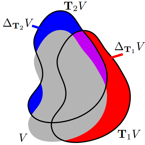
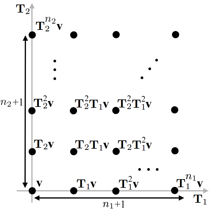
Figure 2: Top: Illustration of the proof intuition. The area of $V$ ($\dim V$) cannot be greater than the product of the height ($\Delta_{\mathbf{T}_{1}}V$) and the width ($\Delta_{\mathbf{T}_{2}}V$). Bottom: Illustration of $W=\mathrm{span}\left\{\mathbf{T}_{2}^{\alpha_{2}}\mathbf{T}_{1}^{\alpha_{1}}\mathbf{v}\,:\,0\leq\alpha_{1}\leq n_{1},0\leq\alpha_{2}\leq n_{2}\right\}$.

We next provide an approximate proof which formalizes this intuition. Before that, we first prove a technical lemma regarding the alignment width of a subspace. The lemma shows that when we perform successive extensions (contractions) of a subspace, the dimension of the resultant subspace increases (decreases) as a concave (convex) function of the number of extensions (contractions).

Lemma 4.

For any diagonal matrix $\mathbf{T}$ and subspace $V$,

$$\Delta_{\mathbf{T}}\left(\mathrm{e}_{\mathbf{T}}V\right)\leq\Delta_{\mathbf{T}}V,$$

$$\Delta_{\mathbf{T}}\left(\mathrm{c}_{\mathbf{T}}V\right)\leq\Delta_{\mathbf{T}}V.$$

Proof:

Note that

$$\Delta_{\mathbf{T}}\left(\mathrm{e}_{\mathbf{T}}V\right)-\Delta_{\mathbf{T}}V$$

$$=\dim\left(\mathbf{T}^{2}V+\mathbf{T}V+V\right)-2\dim\left(\mathbf{T}V+V\right)+\dim V$$

$$=\dim\left(\mathbf{T}^{2}V+\mathbf{T}V\right)+\dim\left(\mathbf{T}V+V\right)$$

$$\quad-\dim\left(\left(\mathbf{T}^{2}V+\mathbf{T}V\right)\cap\left(\mathbf{T}V+V\right)\right)$$

$$\quad-2\dim\left(\mathbf{T}V+V\right)+\dim V$$

$$=\dim V-\dim\left(\left(\mathbf{T}^{2}V+\mathbf{T}V\right)\cap\left(\mathbf{T}V+V\right)\right)\leq 0,$$

where the second to last line follows from (4) and the last line follows from $\dim\left(\left(\mathbf{T}^{2}V+\mathbf{T}V\right)\cap\left(\mathbf{T}V+V\right)\right)\geq\dim(\mathbf{T}V)=\dim V$. A similar result holds for $\Delta_{\mathbf{T}}\left(\mathrm{c}_{\mathbf{T}}V\right)$. ∎

Again when $K\geq 4$, we have at least two matrices $\mathbf{T}_{1}$ and $\mathbf{T}_{2}$, and we will use only these two matrices. The idea of the proof is to find a vector $\mathbf{v}\in V$ and integers $n_{1},n_{2}$ which are large when $\epsilon$ is small such that the space

$$W =\mathrm{e}_{\mathbf{T}_{2}}^{n_{2}}\mathrm{e}_{\mathbf{T}_{1}}^{n_{1}}\left\langle\mathbf{v}\right\rangle$$

$$=\mathrm{span}\left\{\mathbf{T}_{2}^{\alpha_{2}}\mathbf{T}_{1}^{\alpha_{1}}\mathbf{v}\,:\,0\leq\alpha_{1}\leq n_{1},0\leq\alpha_{2}\leq n_{2}\right\}$$

is a proper subspace of $\mathbb{R}^{L}$. By the linear independence condition of $\mathbf{T}_{1}$ and $\mathbf{T}_{2}$, we can then have $(n_{1}+1)(n_{2}+1)<L$ which will allow us to obtain a lower bound bound for $L$ in terms of epsilon. We can think of $W$ as the span of the “grid points” in the rectangle $\left\{0,...,n_{1}\right\}\times\left\{0,...,n_{2}\right\}$. An illustration of the idea is given in Figure 2.

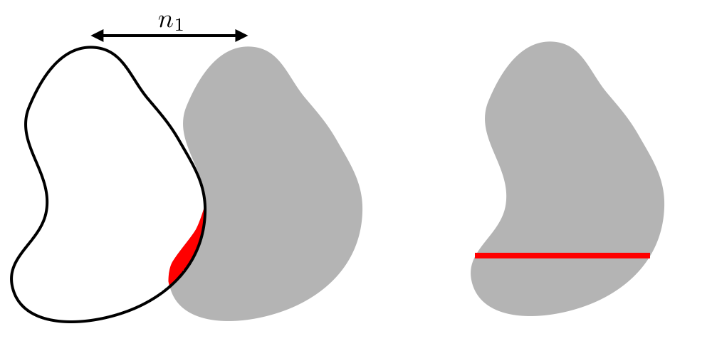
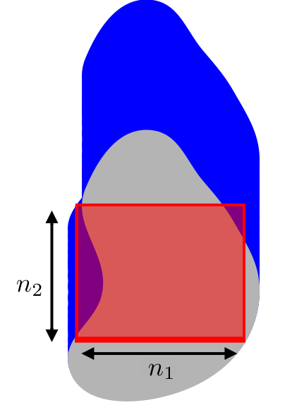
Figure 3: Proof intuition: If $\Delta_{\mathbf{T}_{1}}V$ and $\Delta_{\mathbf{T}_{2}}V$ are both small then a set of vectors $\left\{\mathbf{T}_{2}^{\alpha_{2}}\mathbf{T}_{1}^{\alpha_{1}}\mathbf{v}\,:\,0\leq\alpha_{1}\leq n_{1},0\leq\alpha_{2}\leq n_{2}\right\}$ spans a proper subspace of $\mathbb{R}^{L}$ for some large $n_{1}$ and $n_{2}$.

We will first find a long “line” $\mathrm{e}_{\mathbf{T}_{1}}^{n_{1}}\left\langle\mathbf{v}\right\rangle$ which is a subspace of $V$. Note that if we perform a contraction in $\mathbf{T}_{1}$ direction, the resultant subspace $\mathrm{c}_{\mathbf{T}_{1}}V$, compared to $V$, will have dimension reduced by $\Delta_{\mathbf{T}_{1}}V$. If we perform a second contraction, by Lemma 4, the resultant subspace $\mathrm{c}_{\mathbf{T}_{1}}^{2}V$, will have dimension reduced by at most $\Delta_{\mathbf{T}_{1}}V$ as compared to $\mathrm{c}_{\mathbf{T}_{1}}V$, therefore at most $2\Delta_{\mathbf{T}_{1}}V$ as compared to $V$. Following in this manner, this means that as long as $n_{1}\Delta_{\mathbf{T}_{1}}V<\dim V$, the resultant subspace $\mathrm{c}_{\mathbf{T}_{1}}^{n_{1}}V$ after we perform $n_{1}$ contractions will still be nonempty. Hence we can find

$$\widetilde{\mathbf{v}}\in\mathrm{c}_{\mathbf{T}_{1}}^{n_{1}}V=V\cap\mathbf{T}_{1}V\cap\cdots\cap\mathbf{T}_{1}^{n_{1}}V.$$

This means $\widetilde{\mathbf{v}},\mathbf{T}_{1}^{-1}\widetilde{\mathbf{v}},...,\mathbf{T}_{1}^{-n_{1}}\widetilde{\mathbf{v}}\in V$. Let $\mathbf{v}=\mathbf{T}_{1}^{-n_{1}}\widetilde{\mathbf{v}}$, then $\mathrm{e}_{\mathbf{T}_{1}}^{n_{1}}\left\langle\mathbf{v}\right\rangle\subseteq V$.

Next we find $n_{2}$. Again we know the dimension of $\mathrm{e}_{\mathbf{T}_{2}}V$ is larger by $\Delta_{\mathbf{T}_{2}}V$ as compared to $V$, and moreover by Lemma 4 if we perform multiple extensions the dimension of the resultant subspace increases by at most $\Delta_{\mathbf{T}_{2}}V$ at each step. Hence, as long as $n_{2}\Delta_{\mathbf{T}_{2}}V<L-\dim V$, we can perform $n_{2}$ extensions and the resultant subspace $\mathrm{e}_{\mathbf{T}_{2}}^{n_{2}}V$ will still be a proper subspace of $\mathbb{R}^{L}$. Since $W=\mathrm{e}_{\mathbf{T}_{2}}^{n_{1}}\mathrm{e}_{\mathbf{T}_{1}}^{n_{2}}\left\langle\mathbf{v}\right\rangle\subseteq\mathrm{e}_{\mathbf{T}_{2}}^{n_{2}}V$, $W$ is also a proper subspace of $\mathbb{R}^{L}$.

We finally use the linear independence condition for $\mathbf{T}_{1}$ and $\mathbf{T}_{2}$ to conclude that for any $n_{1}$ and $n_{2}$ such that $n_{1}\Delta_{\mathbf{T}_{1}}V<\dim V$ and $n_{2}\Delta_{\mathbf{T}_{2}}V<L-\dim V$, $(n_{1}+1)(n_{2}+1)<L$. Now, since $\Delta_{\mathbf{T}_{2}}V,\Delta_{\mathbf{T}_{1}}V\leq 2\epsilon L$ and $\dim V=(1-\epsilon)L/2$, we can take any $n_{1}$ and $n_{2}$ such that

$$n_{1} <\dim V/\Delta_{\mathbf{T}_{1}}V=(1-\epsilon)/4\epsilon\approx 1/4\epsilon,$$

$$n_{2} <\left(L-\dim V\right)/\Delta_{\mathbf{T}_{2}}V=(1+\epsilon)/4\epsilon\approx 1/4\epsilon,$$

which gives the lower bound $L\gtrapprox\epsilon^{-2}/16$ on the channel diversity $L$ in terms of the gap $\epsilon$ to the optimal degrees of freedom. Note that the smaller $\epsilon$ we want to achieve, the larger $L$ we need. Equivalently, $\epsilon\geq 1/4\sqrt{L}$. This proof idea is illustrated pictorially in Figure 3.

A few details are missing in this proof intuition. For example, the entries of $\mathbf{v}$ may be zero, so $\dim W$ may be smaller than $(n_{1}+1)(n_{2}+1)$. This is where we need to control the sparsity of the subspace $V$. A rigorous proof is given in the next subsection.

V-B Proof of Theorem 1

In this subsection, we give the proof of Theorem 1, which is implied by the following theorem.

Theorem 4.

Let $\mathbf{T}_{1},\mathbf{T}_{2}\in\mathbb{R}^{L\times L}$ satisfy the linear independence condition. Let $\epsilon>0$. Assume there exist vector subspace $V\subseteq\mathbb{R}^{L}$ with $\dim V=D=\left(1-\epsilon\right)L/2$ satisfying $\mathrm{sp}_{N}\left(V\right)\geq 2N-\epsilon L$ for any $N=1,...,D$, and $\Delta_{\mathbf{T}_{1}}V,\Delta_{\mathbf{T}_{2}}V\leq 2\epsilon L$, then we have

$$L\geq\epsilon^{-2}/121.$$

Proof:

Note that for any $n_{1}\geq 0$, by Lemma 4,

$$\dim\mathrm{c}_{\mathbf{T}_{1}}^{n_{1}}V\geq\dim V-n_{1}\Delta_{\mathbf{T}_{1}}V.$$

Substitute $n_{1}=\left\lfloor\frac{D-N}{2\epsilon L}\right\rfloor$ for some $N$. Since $\Delta_{\mathbf{T}_{1}}V\leq 2\epsilon L$, we have $\dim\mathrm{c}_{\mathbf{T}_{1}}^{n_{1}}V\geq N$, and therefore since $\mathrm{c}_{\mathbf{T}_{1}}^{n_{1}}V\subseteq V$, by the definition of sparsity for $V$, we can find $\left\|\mathbf{v}\right\|_{0}\geq\mathrm{sp}_{N}\left(V\right)$ such that $\mathbf{v}\in\mathbf{T}_{1}^{-n_{1}}\mathrm{c}_{\mathbf{T}_{1}}^{n_{1}}V=\mathrm{c}_{\mathbf{T}_{1}^{-1}}^{n_{1}}V$, and hence $\mathrm{e}_{\mathbf{T}_{1}}^{n_{1}}\left\langle\mathbf{v}\right\rangle\subseteq V$ by (6).

On the other hand, for any $n_{2}\geq 0$, by Lemma 4,

$$\dim\mathrm{e}_{\mathbf{T}_{2}}^{n_{2}}V\leq\dim V+n_{2}\Delta_{\mathbf{T}_{2}}V.$$

Substitute $n_{2}=\left\lfloor\frac{\mathrm{sp}_{N}\left(V\right)-1-D}{2\epsilon L}\right\rfloor$, since $\Delta_{\mathbf{T}_{2}}V\leq 2\epsilon L$, we have $\dim\mathrm{e}_{\mathbf{T}_{2}}^{n_{2}}V\leq\mathrm{sp}_{N}\left(V\right)-1$. Since $\mathrm{e}_{\mathbf{T}_{2}}^{n_{2}}\mathrm{e}_{\mathbf{T}_{1}}^{n_{1}}\left\langle\mathbf{v}\right\rangle\subseteq\mathrm{e}_{\mathbf{T}_{2}}^{n_{2}}V$, we also have $\dim\mathrm{e}_{\mathbf{T}_{2}}^{n_{2}}\mathrm{e}_{\mathbf{T}_{1}}^{n_{1}}\left\langle\mathbf{v}\right\rangle\leq\mathrm{sp}_{N}\left(V\right)-1$.

Note that by the linear independence condition

$$\dim\mathrm{e}_{\mathbf{T}_{1}}^{n_{1}}\mathrm{e}_{\mathbf{T}_{2}}^{n_{2}}\left\langle\mathbf{v}\right\rangle$$

$$=\dim\mathrm{span}\left\{\mathbf{T}_{1}^{\alpha_{1}}\mathbf{T}_{2}^{\alpha_{2}}\mathbf{v}\,:\,0\leq\alpha_{1}\leq n_{1},0\leq\alpha_{2}\leq n_{2}\right\}$$

$$=\min\left\{\left(n_{1}+1\right)\left(n_{2}+1\right),\,\left\|\mathbf{v}\right\|_{0}\right\}.$$

Since $\left\|\mathbf{v}\right\|_{0}\geq\mathrm{sp}_{N}\left(V\right)$ and $\dim\mathrm{e}_{\mathbf{T}_{2}}^{n_{2}}\mathrm{e}_{\mathbf{T}_{1}}^{n_{1}}\left\langle\mathbf{v}\right\rangle\leq\mathrm{sp}_{N}\left(V\right)-1$, $\dim\mathrm{e}_{\mathbf{T}_{2}}^{n_{2}}\mathrm{e}_{\mathbf{T}_{1}}^{n_{1}}\left\langle\mathbf{v}\right\rangle=\left(n_{1}+1\right)\left(n_{2}+1\right)$. Hence we have

$$\mathrm{sp}_{N}\left(V\right)-1 \geq \left(n_{1}+1\right)\left(n_{2}+1\right)$$

$$\geq \left(\frac{D-N}{2\epsilon L}\right)\left(\frac{\mathrm{sp}_{N}\left(V\right)-D}{2\epsilon L}\right),$$

$$4\epsilon^{2}L^{2} \geq \frac{\left(D-N\right)\left(\mathrm{sp}_{N}\left(V\right)-D\right)}{\mathrm{sp}_{N}\left(V\right)-1}$$

$$\geq \frac{\left(D-N\right)\left(\mathrm{sp}_{N}\left(V\right)-D\right)}{\mathrm{sp}_{N}\left(V\right)}.$$

Recall that $D=\left(1-\epsilon\right)L/2$. Substitute $N=\left\lceil\frac{3+\epsilon}{8}L\right\rceil$. Note that $\mathrm{sp}_{N}\left(V\right)\geq 2N-\epsilon L\geq\frac{3}{2}D$.

$$4\epsilon^{2}L^{2} \geq \frac{\left(D-N\right)\left(\mathrm{sp}_{N}\left(V\right)-D\right)}{\mathrm{sp}_{N}\left(V\right)}$$

$$\geq \frac{1}{3}\left(\frac{1-\epsilon}{2}L-\frac{3+\epsilon}{8}L-1\right)$$

$$= \frac{1-5\epsilon}{24}L-\frac{1}{3}.$$

Note that $2D=\left(1-\epsilon\right)L<L$, and since both sides are integers, $2D\leq L-1$ and $L\epsilon\geq 1$. We split the analysis into two cases: if $\epsilon\geq 1/121$, then $L\geq\epsilon^{-1}\geq\frac{1}{121\epsilon^{2}}$; if $\epsilon<1/121$, then $L\geq\epsilon^{-1}>121$. If $L\geq 122$ then

$$4\epsilon^{2}L^{2} \geq \frac{1-5\epsilon}{24}L-\frac{1}{3}$$

$$\geq \frac{1-5\epsilon}{24}L-\frac{L}{366}$$

$$= \frac{57-305\epsilon}{1464}L$$

$$\geq \frac{57-305/121}{1464}L$$

$$= \frac{824}{22143}L.$$

Hence

$$L\geq\frac{206}{22143\epsilon^{2}}\geq\frac{1}{121\epsilon^{2}}.$$

This completes the proof of the theorem. ∎

VI Generalization to Block Fading

In this section, we consider the block fading case, where the channel coefficients are constant over $L$ coherence periods of duration $T$. Let $\mathbf{H}_{ij}=\mathrm{diag}\left[h_{ij}^{(1)},...,h_{ij}^{(L)}\right]\otimes\mathbf{I}_{T}\in\mathbb{R}^{TL\times TL}$, where $\otimes$ denotes the Kronecker product.

Define $\mathbf{P}_{k}\in\mathbb{R}^{T\times TL}$ such that $\left(\mathbf{P}_{k}\right)_{ij}=1$ when $j=T\left(k-1\right)+i$, $\left(\mathbf{P}_{k}\right)_{ij}=0$ otherwise. Note that $\mathbf{P}_{k}$ is the projection which selects the entries of a vector in $\mathbb{R}^{TL}$ that are in the $k$-th coherence period.

It is easy to observe that the width requirement for decoding remains the same in this case, i.e., if $D=\left(1-\epsilon\right)TL/2$ and $V_{i}\subseteq\mathbb{R}^{TL},\,i=1,\dots,K$ satisfy the decoding condition at all the receivers, then $\Delta_{\mathbf{T}_{ijk}}V_{i}\leq 2\epsilon TL$ for all distinct $i,j,k\neq 1$ and again focusing on a single subspace $V=V_{2}$, we have $\Delta_{\mathbf{T}_{i}}V\leq 2\epsilon TL,\,\,\forall i=1,...,M$ where $M=\left(K-2\right)\left(K-3\right)$.

We will need to generalize the definition of sparsity for $V\subseteq\mathbb{R}^{TL}$ as follows. Let

$$\mathrm{sp}^{(T)}\left(V\right)=\sum_{k=1}^{L}\dim\left(\mathbf{P}_{k}V\right),$$

$$\mathrm{sp}^{(T)}_{N}\left(V\right)$$ (7)

$$\!\!=\!\! \!\!\min\left\{\sum_{k=1}^{L}\!\dim\widetilde{W}_{k}:\widetilde{W}_{k}\!\subseteq\!\mathbb{R}^{T}\!,\dim\left(\!V\!\cap\!\sum_{k=1}^{L}\mathbf{P}_{k}^{T}\widetilde{W}_{k}\right)\!\geq\!N\!\right\}$$

$$\!\!=\!\! \!\!\min\left\{\mathrm{sp}^{(T)}\left(W\right)\,:\,W\subseteq V,\,\dim\left(W\right)\geq N\right\}.$$

Note that when $T=1$, $\mathrm{sp}^{(T)}\left(W\right)$ counts the number of positions where the vectors in $W$ have non-zero entries, i.e., $\mathrm{sp}^{(1)}\left(W\right)=\max_{\mathbf{v}\in W}\left\|\mathbf{v}\right\|_{0}$, therefore the new definition of $N$-sparsity coincides with the earlier one in this case. Note that for larger $T$, we consider the dimension of each $T$-length portion of $W$, $\dim\left(\mathbf{P}_{k}W\right)$, instead of simply counting the positions with non-zero entries.

We can observe the following properties for $\mathrm{sp}^{(T)}_{N}\left(V\right)$, which will be used in the following section:

$$\mathrm{sp}^{(T)}_{N}\left(\mathrm{c}_{\mathbf{T}}V\right)\geq\mathrm{sp}^{(T)}_{N}\left(V\right),$$ (8)

$$\mathrm{sp}^{(T)}_{N+\Delta_{\mathbf{T}}V}\left(\mathrm{e}_{\mathbf{T}}V\right)\geq\mathrm{sp}^{(T)}_{N}\left(V\right),$$ (9)

for any diagonal matrix $\mathbf{T}\in\mathbb{R}^{TL\times TL}$. The first inequality simply follows from the fact that $\mathrm{c}_{\mathbf{T}}V\subseteq V$. The second inequality follows from the fact that if there exists $\widetilde{W}_{k}\subseteq\mathbb{R}^{T}$, $W=\sum_{k=1}^{L}\mathbf{P}_{k}^{T}\widetilde{W}_{k}$ such that $\dim(\mathrm{e}_{\mathbf{T}}V\cap W)\geq N+\Delta_{\mathbf{T}}V$ then $\dim(V\cap W)\geq N$. Therefore, $\mathrm{sp}^{(T)}_{N+\Delta_{\mathbf{T}}V}\left(\mathrm{e}_{\mathbf{T}}V\right)\geq\mathrm{sp}^{(T)}_{N}\left(V\right)$.

The following lemma is the analogue of Lemma 2 and establishes the corresponding sparsity requirement for the block fading case.

Lemma 5 (Sparsity requirement for decoding).

If $D=\left(1-\epsilon\right)TL/2$ and $V_{i},\,i=1,\dots,K$ satisfy the decoding condition at all the receivers, then $\mathrm{sp}^{(T)}_{N}\left(V_{i}\right)\geq 2N-\epsilon TL$ for all $i$ and $N=1,...,D$.

Proof:

Assume the contrary that $\mathrm{sp}^{(T)}_{N}\left(V_{i}\right)<2N-\epsilon TL$ for some $N=1,...,D$. This implies that there exists $\widetilde{W}_{k}\subseteq\mathbb{R}^{T}$, $W=\sum_{k=1}^{L}\mathbf{P}_{k}^{T}\widetilde{W}_{k}$ such that $\dim W<2N-\epsilon TL$ and $\dim\left(V_{i}\cap W\right)\geq N$, or equivalently $2\dim\left(V_{i}\cap W\right)-\dim W>\epsilon TL$. Consider the signal at receiver $i$, which is $\mathbf{H}_{ii}V_{i}$, and the interference from transmitter 1 (assume $i$ is not 1 or 2), which is $\mathbf{H}_{i1}V_{1}$. From the decoding condition at receiver $i$, we have $\mathbf{H}_{ii}V_{i}\cap\mathbf{H}_{i1}V_{1}=\{0\}$, $V_{1}\cap\mathbf{H}_{i1}^{-1}\mathbf{H}_{ii}V_{i}=\{0\}$. Note that

$$\mathbf{H}_{ij}W =\sum_{k=1}^{L}\mathbf{H}_{ij}\mathbf{P}_{k}^{T}\widetilde{W}_{k}$$

$$=\sum_{k=1}^{L}\left(\left(\mathbf{H}_{ij}\right)_{T(k-1)+1,\,T(k-1)+1}\mathbf{I}\right)\mathbf{P}_{k}^{T}\widetilde{W}_{k}$$

$$=\sum_{k=1}^{L}\mathbf{P}_{k}^{T}\widetilde{W}_{k}$$

$$=W,$$

and hence,

$$\dim\left(\left(\mathbf{H}_{i1}^{-1}\mathbf{H}_{ii}V_{i}\right)\cap W\right) =\dim\left(V_{i}\cap\left(\mathbf{H}_{i1}\mathbf{H}_{ii}^{-1}W\right)\right)$$

$$=\dim\left(V_{i}\cap W\right)$$

$$>\left(\dim W+\epsilon TL\right)/2.$$

Combining this with $V_{1}\cap\mathbf{H}_{i1}^{-1}\mathbf{H}_{ii}V_{i}=\{0\}$, we have $\dim\left(V_{1}\cap W\right)<\left(\dim W-\epsilon TL\right)/2$.

Consider the interference at receiver 2, we have $\dim\left(\mathbf{H}_{21}V_{1}+\mathbf{H}_{2i}V_{i}\right)=\dim\left(V_{1}+\mathbf{H}_{21}^{-1}\mathbf{H}_{2i}V_{i}\right)\leq\left(1+\epsilon\right)TL/2$, but

$$\dim\left(V_{1}+\mathbf{H}_{21}^{-1}\mathbf{H}_{2i}V_{i}\right)$$

$$\geq\!\!\!\!\! \dim\left(V_{1}+\left(\left(\mathbf{H}_{21}^{-1}\mathbf{H}_{2i}V_{i}\right)\cap W\right)\right)$$

$$>\!\!\!\!\! D\!+\!\left(\dim W+\epsilon TL\right)/2\!-\dim\left(V_{1}\cap\left(\left(\mathbf{H}_{21}^{-1}\mathbf{H}_{2i}V_{i}\right)\cap W\right)\right)$$

$$>\!\!\!\!\! \left(1-\epsilon\right)TL/2+\left(\dim W+\epsilon TL\right)/2-\left(\dim W-\epsilon TL\right)/2$$

$$=\!\!\!\!\! \left(1+\epsilon\right)TL/2,$$

which leads to a contradiction. ∎

We next generalize the linear independence condition for diagonal matrices which we defined in the earlier section to a block linear independence condition. One can again verify that the new condition reduces to the linear independence condition in the earlier section when $T=1$.

Definition 5.

We call a set of diagonal matrices $\left\{\mathbf{T}_{i}\right\}_{i=1,...,M}\subseteq\mathbb{R}^{TL\times TL}$ with nonzero diagonal entries, where $\mathbf{T}_{i}=\widetilde{\mathbf{T}}_{i}\otimes\mathbf{I}_{T}$, satisfies the block linear independence condition if for any set of integer vectors $A\subseteq\mathbb{Z}^{M}$ with $\left|A\right|=L$, and $V\subseteq\mathbb{R}^{TL}$, we have

$$\dim\left(\sum_{\mathbf{x}\in A}\left(\left(\prod_{i=1}^{M}\mathbf{T}_{i}^{x_{i}}\right)V\right)\right)=\mathrm{sp}^{(T)}\left(V\right).$$

Almost all of the sets of diagonal matrices satisfy the block linear independence condition, as shown in the following lemma.

Lemma 6.

Let $\mathbf{T}_{i}\in\mathbb{R}^{TL\times TL}$ ($i=1,...,M$, $M\geq 2$) be diagonal matrices where $\mathbf{T}_{i}=\widetilde{\mathbf{T}}_{i}\otimes\mathbf{I}_{T}$. Consider the $LM$-dimensional space containing all such $\left\{\mathbf{T}_{i}\right\}$ with the Lebesgue measure. Then $\left\{\mathbf{T}_{i}\right\}$ satisfies the block linear independence condition almost everywhere.

Proof:

Let $A=\left\{\mathbf{x}_{1},...,\mathbf{x}_{L}\right\}$, and $\widetilde{\Phi}\left(\mathbf{x}\right)=\prod_{i=1}^{M}\widetilde{\mathbf{T}}_{i}^{x_{i}}$. As shown in Lemma 3, the matrix $\mathbf{X}=\left[\mathrm{diag}\left(\widetilde{\Phi}\left(\mathbf{x}_{1}\right)\right)\,\cdots\,\mathrm{diag}\left(\widetilde{\Phi}\left(\mathbf{x}_{L}\right)\right)\right]$ is full rank for any $A$ almost everywhere. Hence

$$\sum_{\mathbf{x}\in A}\left(\left(\prod_{i=1}^{M}\mathbf{T}_{i}^{x_{i}}\right)V\right)$$

$$=\sum_{i=1}^{L}\left(\widetilde{\Phi}\left(\mathbf{x}_{i}\right)\otimes\mathbf{I}_{T}\right)V$$

$$=\sum_{i=1}^{L}\left(\sum_{j=1}^{L}\left(\mathbf{X}^{-1}\right)_{ij}\left(\widetilde{\Phi}\left(\mathbf{x}_{j}\right)\otimes\mathbf{I}_{T}\right)\right)V$$

$$=\sum_{i=1}^{L}\left(\left(\sum_{j=1}^{L}\left(\mathbf{X}^{-1}\right)_{ij}\widetilde{\Phi}\left(\mathbf{x}_{j}\right)\right)\otimes\mathbf{I}_{T}\right)V$$

$$=\sum_{i=1}^{L}\left(\mathbf{D}_{i}\otimes\mathbf{I}_{T}\right)V$$

$$=\sum_{i=1}^{L}\mathbf{P}_{i}^{T}\mathbf{P}_{i}V,$$

where $\mathbf{D}_{i}\in\mathbb{R}^{L\times L}$ is the diagonal matrix with 1 at the $i$-th position and 0 elsewhere, and $\mathbf{X}^{-1}$ denotes the inverse of the matrix $\mathbf{X}$. Note that each of $\mathbf{P}_{i}^{T}\mathbf{P}_{i}V$ has disjoint support, and therefore

$$\dim\left(\sum_{\mathbf{x}\in A}\left(\left(\prod_{i=1}^{M}\mathbf{T}_{i}^{x_{i}}\right)V\right)\right) =\dim\left(\sum_{i=1}^{L}\mathbf{P}_{i}^{T}\mathbf{P}_{i}V\right)$$

$$=\sum_{i=1}^{L}\dim\left(\mathbf{P}_{i}^{T}\mathbf{P}_{i}V\right)$$

$$=\mathrm{sp}^{(T)}\left(V\right).$$

∎

Theorem 2 follows immediately from the following theorem.

Theorem 5.

Let $\mathbf{T}_{1},\mathbf{T}_{2}\in\mathbb{R}^{TL\times TL}$ satisfy the block linear independence condition. Let $\epsilon>0$. Assume there exist vector subspace $V\subseteq\mathbb{R}^{TL}$ with $\dim V=D=\left(1-\epsilon\right)TL/2$ satisfying $\mathrm{sp}^{(T)}_{N}\left(V\right)\geq 2N-\epsilon TL$ for any $N$, and $\Delta_{\mathbf{T}_{1}}V,\Delta_{\mathbf{T}_{2}}V\leq 2\epsilon TL$, then we have

$$L\geq\epsilon^{-2}/400.$$

Proof:

Note that for any $n_{1}\geq 0$, by Lemma 4,

$$\dim\mathrm{c}_{\mathbf{T}_{1}}^{n_{1}}V\geq\dim V-n_{1}\Delta_{\mathbf{T}_{1}}V.$$

Let $W=\mathbf{T}_{1}^{-n_{1}}\mathrm{c}_{\mathbf{T}_{1}}^{n_{1}}V=\mathrm{c}_{\mathbf{T}_{1}^{-1}}^{n_{1}}V$. Substitute $n_{1}=\left\lfloor\frac{D-N}{2\epsilon TL}\right\rfloor$ for some $N$, we have $\dim W\geq N$, and therefore since $W\subseteq V$, by the definition of sparsity for $V$, $\mathrm{sp}^{(T)}\left(W\right)\geq\mathrm{sp}^{(T)}_{N}\left(V\right)$. Also note that $\mathrm{e}_{\mathbf{T}_{1}}^{n_{1}}W\subseteq V$ by (6).

On the other hand, for any $n_{2}\geq 0$, by Lemma 4,

$$\dim\mathrm{e}_{\mathbf{T}_{2}}^{n_{2}}V\leq\dim V+n_{2}\Delta_{\mathbf{T}_{2}}V.$$

Substitute $n_{2}=\left\lfloor\frac{\mathrm{sp}^{(T)}_{N}\left(V\right)-1-D}{2\epsilon TL}\right\rfloor$, we have $\dim\mathrm{e}_{\mathbf{T}_{2}}^{n_{2}}V\leq\mathrm{sp}^{(T)}_{N}\left(V\right)-1$. Since $\mathrm{e}_{\mathbf{T}_{1}}^{n_{1}}\mathrm{e}_{\mathbf{T}_{2}}^{n_{2}}W\subseteq\mathrm{e}_{\mathbf{T}_{2}}^{n_{2}}V$, we also have $\dim\mathrm{e}_{\mathbf{T}_{1}}^{n_{1}}\mathrm{e}_{\mathbf{T}_{2}}^{n_{2}}W\leq\mathrm{sp}^{(T)}_{N}\left(V\right)-1$.

Note that by the block linear independence condition, if $\left(n_{1}+1\right)\left(n_{2}+1\right)\geq L$, then $\dim\mathrm{e}_{\mathbf{T}_{1}}^{n_{1}}\mathrm{e}_{\mathbf{T}_{2}}^{n_{2}}W\geq\mathrm{sp}^{(T)}_{N}\left(V\right)$, which leads to a contradiction. Hence

$$L > \left(n_{1}+1\right)\left(n_{2}+1\right)$$

$$\geq \left(\frac{D-N}{2\epsilon TL}\right)\left(\frac{\mathrm{sp}^{(T)}_{N}\left(V\right)-D}{2\epsilon TL}\right),$$

$$4\epsilon^{2}T^{2}L^{2} \geq L^{-1}\left(D-N\right)\left(\mathrm{sp}^{(T)}_{N}\left(V\right)-D\right).$$

Recall that $D=\left(1-\epsilon\right)TL/2$. Substitute $N=\left\lceil\frac{3-\epsilon}{8}TL\right\rceil$, by $\mathrm{sp}^{(T)}_{N}\left(V\right)\geq 2N-\epsilon TL$,

$$4\epsilon^{2}T^{2}L^{2} \geq L^{-1}\left(\frac{1-\epsilon}{2}TL-\frac{3-\epsilon}{8}TL-1\right)$$

$$\;\;\;\;\;\;\;\cdot\left(\frac{3-\epsilon}{4}TL-\epsilon TL-\frac{1-\epsilon}{2}TL\right)$$

$$=\frac{1-3\epsilon}{4}T\left(\frac{1-3\epsilon}{8}TL-1\right)$$

$$\geq\frac{\left(1-3\epsilon\right)^{2}}{32}T^{2}L-\frac{1}{4}T.$$

Note that $2D=\left(1-\epsilon\right)TL<TL$, since both sides are integers, $2D\leq TL-1$, $TL\epsilon\geq 1$. If $\epsilon\geq 1/20$, then $L\geq 1\geq\frac{1}{400\epsilon^{2}}$.

If $\epsilon<1/20$, then $TL\geq\epsilon^{-1}>20$, $TL\geq 21$, and

$$4\epsilon^{2}T^{2}L^{2} \geq \frac{\left(1-3\epsilon\right)^{2}}{32}T^{2}L-\frac{1}{4}T$$

$$\geq \frac{\left(1-3/20\right)^{2}}{32}T^{2}L-\frac{T^{2}L}{84}$$

$$= \frac{2869}{268800}T^{2}L.$$

Hence

$$L\geq\frac{2869}{1075200\epsilon^{2}}\geq\frac{1}{400\epsilon^{2}}.$$

∎

VII A Tighter Scaling Bound when $K$ grows

In this section, we prove Theorem 3, which states

$$\mathrm{DoF}\leq\frac{K}{2}\left(1-2^{-17}\min\left\{\frac{1}{\sqrt[4]{L}},\frac{2^{\left(K-2\right)\left(K-3\right)/4}}{\sqrt{L}}\right\}\right).$$

This implies that the gap decreases at most as $1/\sqrt[4]{L}$ when $L$ is smaller than the order of $2^{(K-2)(K-3)}$. We only consider the block fading case in this section, since the fast fading case can be treated as a special case of block fading with $T=1$.

As we have seen in the previous sections, proving that the gap decreases at most as $1/\sqrt{L}$ only requires to use the alignment width condition for two matrices, $\mathbf{T}_{1}$ and $\mathbf{T}_{2}$, one used for extension and one for contraction, i.e., we only need $M\geq 2$. Proving a gap larger than $1/\sqrt{L}$ requires to use more than one matrix for extension and contraction. We believe the proof of this theorem is important in suggesting one way in which this can be done. We introduce the notions of second order extension and contraction widths, which describe how an extension (contraction) in $\mathbf{T}_{2}$ would increase (decrease) the alignment width under $\mathbf{T}_{1}$. This is illustrated in Figure 4.

Definition 6.

(Second order extension and contraction width) For a subspace $V$ and diagonal matrices $\mathbf{T}_{1},\mathbf{T}_{2}$, define the second order extension width $\Delta_{\mathbf{T}_{1},\mathbf{T}_{2}}^{2}V$ and second order contraction width $\nabla_{\mathbf{T}_{1},\mathbf{T}_{2}}^{2}V$ by

$$\Delta_{\mathbf{T}_{1},\mathbf{T}_{2}}^{2}V =\dim\mathrm{e}_{\mathbf{T}_{1}}\mathrm{e}_{\mathbf{T}_{2}}V-\dim\mathrm{e}_{\mathbf{T}_{1}}V-\dim\mathrm{e}_{\mathbf{T}_{2}}V+\dim V$$

$$=\Delta_{\mathbf{T}_{1}}\mathrm{e}_{\mathbf{T}_{2}}V-\Delta_{\mathbf{T}_{1}}V,$$

$$\nabla_{\mathbf{T}_{1},\mathbf{T}_{2}}^{2}V =\dim\mathrm{c}_{\mathbf{T}_{1}}\mathrm{c}_{\mathbf{T}_{2}}V-\dim\mathrm{c}_{\mathbf{T}_{1}}V-\dim\mathrm{c}_{\mathbf{T}_{2}}V+\dim V$$

$$=\Delta_{\mathbf{T}_{1}}V-\Delta_{\mathbf{T}_{1}}\mathrm{c}_{\mathbf{T}_{2}}V.$$

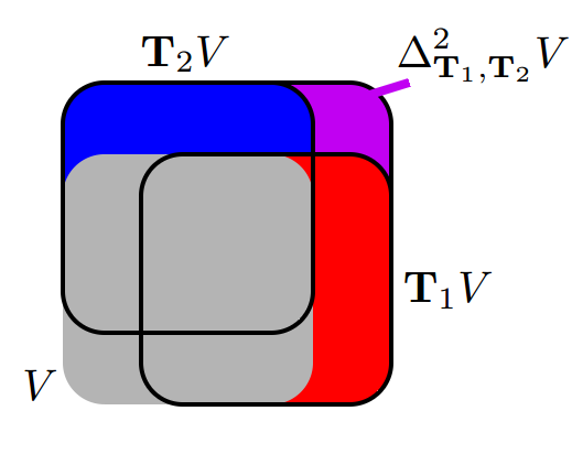
Figure 4: Illustration of the second order extension width of $V$ under $\mathbf{T}_{1},\mathbf{T}_{2}$. Multiplication by $\mathbf{T}_{1}$ and $\mathbf{T}_{2}$ are represented by a shift to the right and upward respectively.

Note that the second order extension and contraction widths can be either positive or negative. An important relation is that

$$\Delta_{\mathbf{T}_{1},\mathbf{T}_{2}}^{2}V\leq\nabla_{\mathbf{T}_{1},\mathbf{T}_{2}}^{2}V,$$ (10)

which follows from (5) by observing that

$$\nabla_{\mathbf{T}_{1},\mathbf{T}_{2}}^{2}V-\Delta_{\mathbf{T}_{1},\mathbf{T}_{2}}^{2}$$

$$=\left(\Delta_{\mathbf{T}_{1}}V-\Delta_{\mathbf{T}_{1}}\mathrm{c}_{\mathbf{T}_{2}}V\right)-\left(\Delta_{\mathbf{T}_{2}}\mathrm{e}_{\mathbf{T}_{1}}V-\Delta_{\mathbf{T}_{2}}V\right)$$

$$=\left(\dim\left(\mathrm{e}_{\mathbf{T}_{1}}V\right)-\dim V-\dim\left(\mathrm{e}_{\mathbf{T}_{1}}\mathrm{c}_{\mathbf{T}_{2}}V\right)+\dim\left(\mathrm{c}_{\mathbf{T}_{2}}V\right)\right)$$

$$\;\;\;-\left(\dim\left(\mathrm{e}_{\mathbf{T}_{1}}V\right)-\dim\left(\mathrm{c}_{\mathbf{T}_{2}}\mathrm{e}_{\mathbf{T}_{1}}V\right)-\dim V+\dim\left(\mathrm{c}_{\mathbf{T}_{2}}V\right)\right)$$

$$=\dim\left(\mathrm{c}_{\mathbf{T}_{2}}\mathrm{e}_{\mathbf{T}_{1}}V\right)-\dim\left(\mathrm{e}_{\mathbf{T}_{1}}\mathrm{c}_{\mathbf{T}_{2}}V\right)$$

$$\geq 0.$$

This implies that for any number $a\geq 0$, either $a\geq\Delta_{\mathbf{T}_{1},\mathbf{T}_{2}}^{2}V$ (i.e., extension of $V$ by $\mathbf{T}_{2}$ increases $\Delta_{\mathbf{T}_{1}}$ by at most $a$), or $a\leq\nabla_{\mathbf{T}_{1},\mathbf{T}_{2}}^{2}V$ (i.e., contraction of $V$ by $\mathbf{T}_{2}$ decreases $\Delta_{\mathbf{T}_{1}}$ by at least $a$) (A respective comment holds when $a\leq 0$.) Intuitively, at least one of contraction or extension by $\mathbf{T}_{2}$ would produce a subspace with small alignment width with respect to $\mathbf{T}_{1}$, i.e. by choosing the respective operation with respect to $\mathbf{T}_{2}$, the new subspace can be made to either have a $\Delta_{\mathbf{T}_{1}}$ which is not much larger than that of the original subspace or even smaller than that.

In Theorem 4, we only use one matrix for extension, and another for contraction. To prove the stronger Theorem 3, we use all the matrices $\mathbf{T}_{1},...,\mathbf{T}_{M}$ (recall $M=\left(K-2\right)\left(K-3\right)$). We consider the average alignment width of a subspace under these matrices. The main idea of the proof is that, we perform extension and contraction repeatedly on the subspace $V$. In each step, we keep the average alignment width small, which guarantees that there exist a matrix among $\mathbf{T}_{1},...,\mathbf{T}_{M}$ with a small alignment width. This matrix is then used for the extension or contraction in the next step.

Definition 7.

(Average alignment width) Define $\overline{\Delta}V=\frac{1}{M}\sum_{j=1}^{M}\Delta_{\mathbf{T}_{j}}V$ to be the average alignment width of subspace $V$ along all $\mathbf{T}_{i}$’s, and similarly define

$$\overline{\Delta}_{\mathbf{T}}^{2}V = \frac{1}{M}\sum_{j=1}^{M}\Delta_{\mathbf{T},\mathbf{T}_{j}}^{2}V,$$

$$\overline{\nabla}_{\mathbf{T}}^{2}V = \frac{1}{M}\sum_{j=1}^{M}\nabla_{\mathbf{T},\mathbf{T}_{j}}^{2}V.$$

By the property of second order alignment width in (10), $\overline{\Delta}_{\mathbf{T}}^{2}V\leq\overline{\nabla}_{\mathbf{T}}^{2}V$. Intuitively, at least one of contraction or extension by $\mathbf{T}$ would produce a subspace with small average alignment width.

As seen in the proof of Theorem 4, our goal is to perform as many extensions on $V$ as possible such that the resultant subspace has dimension less than that of the whole space, and to perform as many contractions on $V$ as possible such that the dimension is greater than 0. The number of consecutive extensions/contractions performed directly affects the bound on $L$. This number is in turn dictated by the alignment width of the subspace, which is the increase in dimension after performing an extension (and the decrease in dimension after performing a contraction), and therefore it determines how many further extensions/contractions can be performed.

We will next present several lemmas which are useful in proving Theorem 3. The following lemma shows that we can either perform extension on a subspace repeatedly to obtain a subspace with similar dimension, sparsity and average alignment width, or find another subspace with smaller average alignment width and similar dimension and sparsity.

The intuition behind this lemma is that we can perform extensions on $W$ using different matrices (unlike Theorem 4 which uses the same matrix repeatedly) to obtain $\mathrm{e}_{\mathbf{T}_{k_{1}}}\cdots\mathrm{e}_{\mathbf{T}_{k_{\tilde{n}-1}}}W$, until the next extension $\mathrm{e}_{\mathbf{T}_{k_{1}}}\cdots\mathrm{e}_{\mathbf{T}_{k_{\tilde{n}}}}W$ would increase the average alignment width too much. If such event does not happen, then we obtain a long series of extensions such that the resultant subspace does not have an average alignment width much larger than the original one. If such an event happens (i.e. the extension $\mathrm{e}_{\mathbf{T}_{k_{\tilde{n}}}}$ increases the average alignment width too much), by the property of second order alignment width in (10), we know that the contraction $\mathrm{c}_{\mathbf{T}_{k_{\tilde{n}}}}$ can be used to significantly decrease the average alignment width. By performing the contraction instead of extension, we break the series of extensions but the average alignment width can now be made smaller than what we started with.

Lemma 7.

Let $\mathbf{T}_{j}\in\mathbb{R}^{TL\times TL}$ ($j=1,...,M$, $M\geq 2$) be diagonal matrices satisfying the block linear independence condition. For any vector subspace $W\subseteq\mathbb{R}^{TL}$, subset $S\subseteq\{1,...,M\}$, and strictly increasing sequence of real numbers $\overline{\Delta}W<a_{1}<\cdots<a_{n}$, $n\geq 0$ (assume $a_{0}=\overline{\Delta}W$), if

$$n\leq\left|S\right|-M/2,$$ (11)

then there exist subspace $\widetilde{W}\subseteq\mathbb{R}^{TL}$ and $\widetilde{n}\in\{0,...,n\}$ such that

$$\left|\dim\widetilde{W}-\dim W\right|\leq\delta,$$ (12)

$$\mathrm{sp}^{(T)}_{\,N+\delta}\left(\widetilde{W}\right)\geq\mathrm{sp}^{(T)}_{N}\left(W\right)$$ (13)

for any $N\geq 0$, where

$$\delta=2\sum_{i=0}^{\widetilde{n}-1}a_{i},$$

and at least one of the following cases holds:

1. We have $\widetilde{n}\geq 1$, and

   $$\overline{\Delta}\widetilde{W}\leq 2a_{\widetilde{n}-1}-a_{\widetilde{n}}.$$ (14)

2. We have $\widetilde{n}=n$,

   $$\overline{\Delta}\widetilde{W}\leq a_{n},$$ (15)

   and there exist distinct $k_{1},...,k_{n}\in S$ such that

   $$\widetilde{W}=\mathrm{e}_{\mathbf{T}_{k_{1}}}\cdots\mathrm{e}_{\mathbf{T}_{k_{n}}}W.$$ (16)

The same lemma also holds when $\widetilde{W}=\mathrm{e}_{\mathbf{T}_{k_{1}}}\cdots\mathrm{e}_{\mathbf{T}_{k_{n}}}W$ is replaced by $\widetilde{W}=\mathrm{c}_{\mathbf{T}_{k_{1}}}\cdots\mathrm{c}_{\mathbf{T}_{k_{n}}}W$. We call the former the extension version of the lemma, and the latter the contraction version.

Proof:

We prove the extension version $\widetilde{W}=\mathrm{e}_{\mathbf{T}_{k_{1}}}\cdots\mathrm{e}_{\mathbf{T}_{k_{n}}}W$ here. The contraction version is similar. We prove the lemma by induction on $n$. Note that when $n=0$, we have $\delta=0$, and $\widetilde{W}=W$, $\widetilde{n}=0$ obviously satisfies (12), (13), (15) and (16). We then consider $n\geq 1$ and assume the lemma is true for $n-1$.

By Markov inequality, we have

$$\left|\left\{j\in\{1,...,M\}\,:\,\Delta_{\mathbf{T}_{j}}W\leq 2\overline{\Delta}W\right\}\right|\geq M/2.$$ (17)

By (11), we have $\left|S\right|>M/2$, hence we can always find $k\in S$ such that $\Delta_{\mathbf{T}_{k}}W\leq 2\overline{\Delta}W$. Consider two cases:

Case 1: $\overline{\Delta}_{\mathbf{T}_{k}}^{2}W>a_{1}-\overline{\Delta}W$,

We will check that $\widetilde{W}=\mathrm{c}_{\mathbf{T}_{k}}W$ and $\widetilde{n}=1$ satisfies (12), (13) and (14). First we bound $\Delta_{\mathbf{T}_{k}}W$ by

$$\Delta_{\mathbf{T}_{k}}W\leq 2\overline{\Delta}W=2a_{0}=2\sum_{i=0}^{\widetilde{n}-1}a_{i}=\delta.$$

For (12), $\dim\widetilde{W}\leq\dim W$, and

$$\dim\widetilde{W} \geq\dim W-\Delta_{\mathbf{T}_{k}}W$$

$$\geq\dim W-\delta.$$

Note that (13) follows directly from (9) and $\Delta_{\mathbf{T}_{k}}W\leq\delta$. Finally for (14),

$$\overline{\Delta}\widetilde{W} =\overline{\Delta}W-\overline{\nabla}_{\mathbf{T}_{k}}^{2}W$$

$$\leq\overline{\Delta}W-\overline{\Delta}_{\mathbf{T}_{k}}^{2}W$$

$$<\overline{\Delta}W-\left(a_{1}-\overline{\Delta}W\right)$$

$$=2a_{0}-a_{1}.$$

Case 2: $\overline{\Delta}_{\mathbf{T}_{k}}^{2}W\leq a_{1}-\overline{\Delta}W$,

Let $\widehat{W}=\mathrm{e}_{\mathbf{T}_{k}}W$. We apply induction hypothesis on the subspace $\widehat{W}$, subset $S\backslash\left\{k\right\}$ and sequence $a_{2},...,a_{n}$. To check (11),

$$n-1 \leq\left|S\right|-1-M/2$$

$$=\left|S\backslash\left\{k\right\}\right|-M/2.$$

Hence there exist $\widetilde{W}$ satisfying (12), (13), and either (14), or both (15) and (16) with $\widehat{W}$, $S\backslash\left\{k\right\}$ and $a_{2},...,a_{n}$. We prove that $\widetilde{W}$ satisfies the requirements for $W$, $S$ and $a_{1},...,a_{n}$ as well.

For (12),

$$\left|\dim\widetilde{W}\!-\dim W\right|\! \leq\left|\dim\widetilde{W}-\dim\widehat{W}\right|+\left|\dim\widehat{W}-\dim W\right|$$

$$\leq 2\left(\overline{\Delta}\widehat{W}+\sum_{i=2}^{\widetilde{n}-1}a_{i}\right)+\Delta_{\mathbf{T}_{k}}W$$

$$=2\left(\overline{\Delta}W+\overline{\Delta}_{\mathbf{T}_{k}}^{2}W+\sum_{i=2}^{\widetilde{n}-1}a_{i}\right)+\Delta_{\mathbf{T}_{k}}W$$

$$\leq 2\left(\overline{\Delta}W+a_{1}-\overline{\Delta}W+\sum_{i=2}^{\widetilde{n}-1}a_{i}\right)+2\overline{\Delta}W$$

$$=2\sum_{i=0}^{\widetilde{n}-1}a_{i}.$$

For (13),

$$\mathrm{sp}^{(T)}_{\,N+2\sum_{i=0}^{\widetilde{n}-1}a_{i}}\left(\widetilde{W}\right) \geq\mathrm{sp}^{(T)}_{N+2\sum_{i=0}^{\widetilde{n}-1}a_{i}-2\left(\overline{\Delta}\widehat{W}+\sum_{i=2}^{\widetilde{n}-1}a_{i}\right)}\left(\widehat{W}\right)$$

$$=\mathrm{sp}^{(T)}_{N+2a_{1}-2\overline{\Delta}\widehat{W}}\left(\widehat{W}\right)$$

$$=\mathrm{sp}^{(T)}_{N+2a_{1}-2\overline{\Delta}W+2\overline{\Delta}_{\mathbf{T}_{k}}^{2}W}\left(\widehat{W}\right)$$

$$\geq\mathrm{sp}^{(T)}_{N}\left(\widehat{W}\right).$$

If (14) is satisfied for $\widehat{W}$, $S\backslash\left\{k\right\}$ and $a_{2},...,a_{n}$, then it is clearly also satisfied for $W$, $S$ and $a_{1},...,a_{n}$ by incrementing $\widetilde{n}$ by one.

If (15) and (16) are satisfied for $\widehat{W}$, $S\backslash\left\{k\right\}$ and $a_{2},...,a_{n}$, then (15) is clearly also satisfied for $W$, $S$ and $a_{1},...,a_{n}$ since $a_{n}$ is the same in both cases. Also (16) directly follows from $\widehat{W}=\mathrm{e}_{\mathbf{T}_{k}}W$.

The result follows from induction. ∎

Next we utilize Lemma 7 repeatedly to show that given a subspace $W$, there exist two subspaces $\widetilde{W}_{1}$ and $\widetilde{W}_{2}$ with similar dimension, sparsity and average alignment width, such that the repeated contraction of one of them contains the other one. The main idea is to apply both the extension and contraction versions of Lemma 7 on $W$. If both versions give a repeated extension and contraction, then those repeated extension and contraction would satisfy the requirement. Otherwise if one of the versions gives a subspace with smaller average alignment width, then we can consider that subspace instead and repeat the process.

Lemma 8.

Let $\mathbf{T}_{j}\in\mathbb{R}^{TL\times TL}$ ($j=1,...,M$, $M\geq 2$) be diagonal matrices satisfying the block linear independence condition. For any vector subspace $W\subseteq\mathbb{R}^{TL}$ and integer $n\in\mathbb{Z}_{\geq 0}$, $n\leq M/4$, there exist subspaces $\widetilde{W}_{1},\widetilde{W}_{2}\subseteq\mathbb{R}^{TL}$ such that

$$\overline{\Delta}\widetilde{W}_{i}\leq 2\overline{\Delta}W,$$ (18)

$$\left|\dim\widetilde{W}_{i}-\dim W\right|\leq\delta,$$ (19)

$$\mathrm{sp}^{(T)}_{\,N+\delta}\left(\widetilde{W}_{i}\right)\geq\mathrm{sp}^{(T)}_{N}\left(W\right)$$ (20)

for any $i\in\{1,2\}$ and $N\geq 0$, where

$$\delta=2^{n+3}\overline{\Delta}W$$

and there exist distinct $k_{1},...,k_{2n}\in\{1,...,M\}$ such that

$$\widetilde{W}_{1}\subseteq\mathrm{c}_{\mathbf{T}_{k_{1}}}\cdots\mathrm{c}_{\mathbf{T}_{k_{2n}}}\widetilde{W}_{2}.$$ (21)

Proof:

We perform induction on $M\overline{\Delta}W$, which is a nonnegative integer. When $\overline{\Delta}W=0$, then $\Delta_{\mathbf{T}_{k}}W=0$ for all $k$. It can be checked easily that $\widetilde{W}_{1}=\widetilde{W}_{2}=W$ satisfies the conditions. Next we assume the lemma is true for all subspaces with average alignment width less than $\overline{\Delta}W$ and show that it holds for $W$ with average alignment width $\overline{\Delta}W$.

We invoke Lemma 7 (extension version) on $W$, $\{1,...,M\}$ and sequence

$$a_{i}=\overline{\Delta}W\cdot\left(1+2^{-(n+1)}\left(2^{i+1}-i-2\right)\right),\,\,i=1,...,n.$$

Note that $a_{i}<2\overline{\Delta}W$. Suppose the lemma gives $\widetilde{W}\subseteq\mathbb{R}^{TL}$ and $\widetilde{n}\in\{0,...,n\}$, which satisfy

$$\left|\dim\widetilde{W}-\dim W\right|\leq 2\sum_{i=0}^{\widetilde{n}-1}a_{i}<4\widetilde{n}\overline{\Delta}W,$$

$$\mathrm{sp}^{(T)}_{\,N+4\widetilde{n}\overline{\Delta}W}\left(\widetilde{W}\right)\geq\mathrm{sp}^{(T)}_{N}\left(W\right)$$

for any $N\geq 0$. Consider two cases of the outcome of the lemma:

Case 1: $\widetilde{n}\geq 1$ and $\overline{\Delta}\widetilde{W}\leq 2a_{\widetilde{n}-1}-a_{\widetilde{n}},$

Note that

$$\overline{\Delta}\widetilde{W} \leq 2a_{\widetilde{n}-1}-a_{\widetilde{n}}$$

$$=\overline{\Delta}W\cdot\bigg{(}2\left(1+2^{-(n+1)}\left(2^{\widetilde{n}}-\widetilde{n}-1\right)\right)$$

$$\;\;\;\;\;\;\;\;\;-\left(1+2^{-(n+1)}\left(2^{\widetilde{n}+1}-\widetilde{n}-2\right)\right)\bigg{)}$$

$$=\overline{\Delta}W\cdot\left(1-2^{-(n+1)}\widetilde{n}\right).$$

Hence $\overline{\Delta}\widetilde{W}<\overline{\Delta}W$. By applying the induction hypothesis on $\widetilde{W}$, we obtain $\widetilde{W}_{1}$ and $\widetilde{W}_{2}$. We will check that they satisfy the conditions.

For (18),

$$\overline{\Delta}\widetilde{W}_{i}\leq 2\overline{\Delta}\widetilde{W}<2\overline{\Delta}W.$$

For (19),

$$\left|\dim\widetilde{W}_{i}\!-\dim W\right|\! \leq\left|\dim\widetilde{W}_{i}-\dim\widetilde{W}\right|+\left|\dim\widetilde{W}-\dim W\right|$$

$$\leq 2^{n+3}\overline{\Delta}\widetilde{W}+4\widetilde{n}\overline{\Delta}W$$

$$\leq 2^{n+3}\overline{\Delta}W\cdot\left(1-2^{-(n+1)}\widetilde{n}\right)+4\widetilde{n}\overline{\Delta}W$$

$$=2^{n+3}\overline{\Delta}W.$$

For (20),

$$\mathrm{sp}^{(T)}_{\,N+\delta}\left(\widetilde{W}_{i}\right) =\mathrm{sp}^{(T)}_{\,N+2^{n+3}\overline{\Delta}W}\left(\widetilde{W}_{i}\right)$$

$$\geq\mathrm{sp}^{(T)}_{\,N+2^{n+3}\overline{\Delta}W-2^{n+3}\overline{\Delta}\widetilde{W}}\left(\widetilde{W}\right)$$

$$\geq\mathrm{sp}^{(T)}_{\,N+4\widetilde{n}\overline{\Delta}W}\left(\widetilde{W}\right)$$

$$\geq\mathrm{sp}^{(T)}_{N}\left(W\right).$$

Note that (21) is satisfied by induction hypothesis.

Case 2: $\widetilde{n}=n$, $\overline{\Delta}\widetilde{W}\leq a_{n},$ and there exist distinct $k_{1},...,k_{n}\in S$ such that $\widetilde{W}=\mathrm{e}_{\mathbf{T}_{k_{1}}}\cdots\mathrm{e}_{\mathbf{T}_{k_{n}}}W$,

We invoke Lemma 7 again, but use the contraction version instead, on $W$, subset $\{1,...,M\}\backslash\{k_{1},...,k_{n}\}$ and the same sequence $a_{1},...,a_{n}$. To check (11),

$$n \leq M/4$$

$$\leq\left|\{1,...,M\}\backslash\{k_{1},...,k_{n}\}\right|-M/2.$$

Suppose the lemma gives $\widetilde{W}^{\prime}\subseteq\mathbb{R}^{TL}$ and $\widetilde{n}^{\prime}\in\{0,...,n\}$, which satisfy

$$\left|\dim\widetilde{W}^{\prime}-\dim W\right|<4\widetilde{n}^{\prime}\overline{\Delta}W,$$

$$\mathrm{sp}^{(T)}_{\,N+4\widetilde{n}^{\prime}\overline{\Delta}W}\left(\widetilde{W}^{\prime}\right)\geq\mathrm{sp}^{(T)}_{N}\left(W\right)$$

for any $N\geq 0$.

If the first case of Lemma 7 holds, then we can show that $\widetilde{W}^{\prime}$ satisfies the conditions by the same arguments as in case 1. Hence we assume the second case holds, that is, $\widetilde{n}^{\prime}=n$, $\overline{\Delta}\widetilde{W}^{\prime}\leq a_{n},$ and there exist distinct $k_{n+1},...,k_{2n}\in S$ such that $\widetilde{W}^{\prime}=\mathrm{c}_{\mathbf{T}_{k_{n+1}}}\cdots\mathrm{c}_{\mathbf{T}_{k_{2n}}}W$. We now check that $\widetilde{W}_{1}=\widetilde{W}^{\prime}$, $\widetilde{W}_{2}=\widetilde{W}$ satisfies the conditions.

For (18),

$$\overline{\Delta}\widetilde{W}_{i} \leq a_{n}$$

$$=\overline{\Delta}W\cdot\left(1+2^{-(n+1)}\left(2^{n+1}-n-2\right)\right)$$

$$<2\overline{\Delta}W.$$

For (19),

$$\left|\dim\widetilde{W}_{i}-\dim W\right| \leq 4n\overline{\Delta}W$$

$$\leq 2^{n+3}\overline{\Delta}W.$$

Similar holds for (20). For (21),

$$\widetilde{W}_{1} =\mathrm{c}_{\mathbf{T}_{k_{n+1}}}\cdots\mathrm{c}_{\mathbf{T}_{k_{2n}}}W$$

$$\subseteq\mathrm{c}_{\mathbf{T}_{k_{n+1}}}\cdots\mathrm{c}_{\mathbf{T}_{k_{2n}}}\left(\mathrm{c}_{\mathbf{T}_{k_{1}}}\cdots\mathrm{c}_{\mathbf{T}_{k_{n}}}\widetilde{W}_{2}\right)$$

$$=\mathrm{c}_{\mathbf{T}_{k_{1}}}\cdots\mathrm{c}_{\mathbf{T}_{k_{2n}}}\widetilde{W}_{2}.$$

This completes the proof of Lemma 8. ∎

Next we present a lemma which uses the resultant subspaces of Lemma 8 to establish a bound on $L$. It is proved in a way similar to Theorem 4 and Theorem 5.

Lemma 9.

Let $\mathbf{T}_{j}\in\mathbb{R}^{TL\times TL}$ ($j=1,...,M$, $M\geq 2$) be diagonal matrices satisfying the block linear independence condition. Let $W_{1},W_{2}\subseteq\mathbb{R}^{TL}$ be subspaces with $\dim W_{1}=D_{1}$, $\dim W_{2}=D_{2}$ satisfying $W_{1}\subseteq\mathrm{c}_{\mathbf{T}_{3}}\mathrm{c}_{\mathbf{T}_{4}}\cdots\mathrm{c}_{\mathbf{T}_{M}}W_{2}$, $\mathrm{sp}^{(T)}_{N}\left(W_{1}\right)\geq 2N-\alpha$ for any $N$, where $\alpha>0$, $D_{1}-D_{2}/2-\alpha/2\geq 4$, and $\Delta_{\mathbf{T}_{1}}W_{1},\,\Delta_{\mathbf{T}_{2}}W_{2}\leq 8\epsilon TL$. Then we have

$$L^{3}\geq 2^{M-10}\epsilon^{-2}T^{-2}\left(D_{1}-D_{2}/2-\alpha/2\right)^{2}.$$

Proof:

Recall that for any $n_{1}\geq 0$,

$$\dim\mathrm{c}_{\mathbf{T}_{1}}^{n_{1}}W_{1}\geq D_{1}-n_{1}\Delta_{\mathbf{T}_{1}}W_{1}.$$

Substitute $n_{1}=\left\lfloor\frac{D_{1}-N}{8\epsilon TL}\right\rfloor$ for some $N$, we have $\dim\mathrm{c}_{\mathbf{T}_{1}}^{n_{1}}W_{1}\geq N$. Let

$$\widehat{W} =\mathbf{T}_{1}^{-n_{1}}\mathbf{T}_{3}^{-1}\cdots\mathbf{T}_{M}^{-1}\mathrm{c}_{\mathbf{T}_{1}}^{n_{1}}W_{1},$$

then

$$\mathrm{e}_{\mathbf{T}_{1}}^{n_{1}}\mathrm{e}_{\mathbf{T}_{3}}\mathrm{e}_{\mathbf{T}_{4}}\cdots\mathrm{e}_{\mathbf{T}_{M}}\widehat{W}$$

$$=\mathrm{e}_{\mathbf{T}_{3}}\mathrm{e}_{\mathbf{T}_{4}}\cdots\mathrm{e}_{\mathbf{T}_{M}}\mathbf{T}_{3}^{-1}\cdots\mathbf{T}_{M}^{-1}\mathrm{e}_{\mathbf{T}_{1}}^{n_{1}}\mathbf{T}_{1}^{-n_{1}}\mathrm{c}_{\mathbf{T}_{1}}^{n_{1}}W_{1}$$

$$\subseteq\mathrm{e}_{\mathbf{T}_{3}}\mathrm{e}_{\mathbf{T}_{4}}\cdots\mathrm{e}_{\mathbf{T}_{M}}\mathbf{T}_{3}^{-1}\cdots\mathbf{T}_{M}^{-1}W_{1}$$

$$\subseteq\mathrm{e}_{\mathbf{T}_{3}}\mathrm{e}_{\mathbf{T}_{4}}\cdots\mathrm{e}_{\mathbf{T}_{M}}\mathbf{T}_{3}^{-1}\cdots\mathbf{T}_{M}^{-1}\mathrm{c}_{\mathbf{T}_{3}}\mathrm{c}_{\mathbf{T}_{4}}\cdots\mathrm{c}_{\mathbf{T}_{M}}W_{2}$$

$$\subseteq W_{2},$$

which follows from the fact that the extension and contraction operations commute among themselves and also with multiplication with diagonal matrices and applying the fact that $\mathbf{T}^{-1}\mathrm{e}_{\mathbf{T}}\mathrm{c}_{\mathbf{T}}W\subseteq W$.

On the other hand, for any $n_{2}\geq 0$,

$$\dim\mathrm{e}_{\mathbf{T}_{2}}^{n_{2}}W_{2}\leq D_{2}+n_{2}\Delta_{\mathbf{T}_{2}}W_{2}.$$

Substitute $n_{2}=\left\lfloor\frac{\mathrm{sp}^{(T)}_{N}\left(W_{1}\right)-1-D_{2}}{8\epsilon TL}\right\rfloor$, we have $\dim\mathrm{e}_{\mathbf{T}_{2}}^{n_{2}}W_{2}\leq\mathrm{sp}^{(T)}_{N}\left(W_{1}\right)-1$. Let

$$\widetilde{W}=\mathrm{e}_{\mathbf{T}_{1}}^{n_{1}}\mathrm{e}_{\mathbf{T}_{2}}^{n_{2}}\mathrm{e}_{\mathbf{T}_{3}}\mathrm{e}_{\mathbf{T}_{4}}\cdots\mathrm{e}_{\mathbf{T}_{M}}\widehat{W}.$$

Since $\widetilde{W}\subseteq\mathrm{e}_{\mathbf{T}_{2}}^{n_{2}}W_{2}$, we also have $\dim\widetilde{W}\leq\mathrm{sp}^{(T)}_{N}\left(W_{1}\right)-1$.

By the fact that $\mathbf{T}_{j}$ satisfy the block linear independence condition in Definition 5, if $2^{M-2}\left(n_{1}+1\right)\left(n_{2}+1\right)\geq L$, then

$$\dim\mathrm{e}_{\mathbf{T}_{1}}^{n_{1}}\mathrm{e}_{\mathbf{T}_{2}}^{n_{2}}\mathrm{e}_{\mathbf{T}_{3}}\mathrm{e}_{\mathbf{T}_{4}}\cdots\mathrm{e}_{\mathbf{T}_{M}}\widehat{W}\,=\,\mathrm{sp}^{(T)}(\widehat{W}).$$

Combining this with the fact that $\dim\widetilde{W}\leq\mathrm{sp}^{(T)}_{N}\left(W_{1}\right)-1$ and that $\mathrm{sp}^{(T)}(\widehat{W})\,\geq\,\mathrm{sp}^{(T)}_{N}\left(W_{1}\right)$, which follows from the definition of $N$-sparsity in (7) combined with $\dim\widehat{W}\geq N$ and $\widehat{W}\subseteq\mathbf{T}_{1}^{-n_{1}}\mathbf{T}_{3}^{-1}\cdots\mathbf{T}_{M}^{-1}W_{1}$, which leads to a contradiction,

$$\mathrm{sp}^{(T)}_{N}\left(W_{1}\right)-1 \geq\,\dim\mathrm{e}_{\mathbf{T}_{1}}^{n_{1}}\mathrm{e}_{\mathbf{T}_{2}}^{n_{2}}\mathrm{e}_{\mathbf{T}_{3}}\mathrm{e}_{\mathbf{T}_{4}}\cdots\mathrm{e}_{\mathbf{T}_{M}}\widehat{W}$$

$$\geq\,\mathrm{sp}^{(T)}_{N}(\widehat{W})\,\geq\,\mathrm{sp}^{(T)}_{N}\left(W_{1}\right).$$

Hence,

$$L > 2^{M-2}\left(n_{1}+1\right)\left(n_{2}+1\right)$$

$$\geq 2^{M-2}\left(\frac{D_{1}-N}{8\epsilon TL}\right)\left(\frac{\mathrm{sp}^{(T)}_{N}\left(W_{1}\right)-D_{2}}{8\epsilon TL}\right),$$

$$\epsilon^{2}T^{2}L^{3} \geq 2^{M-8}\left(D_{1}-N\right)\left(\mathrm{sp}^{(T)}_{N}\left(W_{1}\right)-D_{2}\right).$$

Substitute $N=\biggl{\lceil}D_{1}/2+D_{2}/4+\alpha/4\biggr{\rceil}$. By $\mathrm{sp}^{(T)}_{N}\left(W_{1}\right)\geq 2N-\alpha$, we have

$$\epsilon^{2}T^{2}L^{3} \geq 2^{M-9}\left(D_{1}-D_{2}/2-\alpha/2-2\right)\left(D_{1}-D_{2}/2-\alpha/2\right)$$

$$\geq 2^{M-10}\left(D_{1}-D_{2}/2-\alpha/2\right)^{2},$$

since $D_{1}-D_{2}/2-\alpha/2\geq 4$. ∎

Theorem 3 follows directly from the following theorem.

Theorem 6.

Let $\mathbf{T}_{j}\in\mathbb{R}^{TL\times TL}$ ($j=1,...,M$, $M\geq 2$) be diagonal matrices satisfying the block linear independence condition. If there exist a vector subspace $V\subseteq\mathbb{R}^{TL}$ with $\dim V=\left(1-\epsilon\right)TL/2$ satisfying $\mathrm{sp}^{(T)}_{N}\left(V\right)\geq 2N-\epsilon TL$ for any $N$, and $\Delta_{T_{j}}V\leq 2\epsilon TL$ for any $j$, then we have

$$L\geq 2^{-34}\epsilon^{-2}\min\left\{2^{M/2},\,\epsilon^{-2}\right\},$$

Proof:

If $\epsilon>1/512$, then by Theorem 5,

$$L \geq\epsilon^{-2}/400$$

$$\geq 2^{-34}\epsilon^{-4}$$

$$\geq 2^{-34}\epsilon^{-2}\min\left\{2^{M/2},\,\epsilon^{-2}\right\}.$$

Hence we assume $\epsilon\leq 1/512$ throughout the proof. Note that since $\dim V=(1-\epsilon)TL/2<TL/2$, we have $(1-\epsilon)TL/2\leq(TL-1)/2$, and therefore $TL\geq\epsilon^{-1}\geq 512$.

If $M<8$, then by Theorem 5,

$$L \geq\epsilon^{-2}/400$$

$$\geq 2^{-34}\epsilon^{-2}\cdot 2^{M/2}$$

$$\geq 2^{-34}\epsilon^{-2}\min\left\{2^{M/2},\,\epsilon^{-2}\right\}.$$

Hence we assume $M\geq 8$ throughout the proof.

Note that $\overline{\Delta}V\leq 2\epsilon TL$. We next apply Lemma 8 on $V$ by choosing

$$n=\min\left\{\left\lfloor M/4\right\rfloor-1,\,\left\lfloor\log_{2}(\epsilon^{-1})\right\rfloor-9\right\},$$

(note that $n\geq 0$ since $M\geq 8$ and $\epsilon^{-1}\geq 512$). Lemma 8 guarantees the existences of two subspaces $\widetilde{W}_{1},\widetilde{W}_{2}\subseteq\mathbb{R}^{TL}$ such that $\overline{\Delta}\widetilde{W}_{i}\leq 4\epsilon TL$, and for any $i\in\{1,2\}$ and $N\geq 0$,

$$\left|\dim\widetilde{W}_{i}-\left(1-\epsilon\right)TL/2\right|\leq 2^{n+4}\epsilon TL,$$

$$\mathrm{sp}^{(T)}_{N+2^{n+4}\epsilon TL}\left(\widetilde{W}_{i}\right)\geq\mathrm{sp}^{(T)}_{N}(V),$$

where using $\mathrm{sp}^{(T)}_{N}\left(V\right)\geq 2N-\epsilon TL$, the last inequality implies

$$\mathrm{sp}^{(T)}_{N}\left(\widetilde{W}_{i}\right)\geq 2N-\left(2^{n+5}+1\right)\epsilon TL.$$

By Lemma 8, there also exist distinct $k_{3},...,k_{2n+2}\in\{1,...,M\}$ such that

$$\widetilde{W}_{1}\subseteq\mathrm{c}_{\mathbf{T}_{k_{3}}}\cdots\mathrm{c}_{\mathbf{T}_{k_{2n+2}}}\widetilde{W}_{2}.$$ (22)

Since $M-2n-1>M/2$, by applying the same argument as in (17) twice, we can find $k_{1},k_{2}$ such that $k_{1},k_{2},k_{3},...,k_{2n+2}$ are distinct, $\Delta_{\mathbf{T}_{k_{1}}}\widetilde{W}_{1},\,\Delta_{\mathbf{T}_{k_{2}}}\widetilde{W}_{2}\leq 8\epsilon TL$.

We apply Lemma 9 on $\widetilde{W}_{1}$, $\widetilde{W}_{2}$ and $\mathbf{T}_{k_{1}},....,\mathbf{T}_{k_{2n+2}}$. Let $\alpha=\left(2^{n+5}+1\right)\epsilon TL$. We first check that the condition $\dim\widetilde{W}_{1}-\frac{1}{2}\dim\widetilde{W}_{2}-\frac{\alpha}{2}\geq 4$ required in Lemma 9 is satisfied:

$$\dim\widetilde{W}_{1}-\frac{1}{2}\dim\widetilde{W}_{2}-\frac{1}{2}\left(2^{n+5}+1\right)\epsilon TL$$

$$=\left(\dim\widetilde{W}_{1}-\frac{\left(1-\epsilon\right)TL}{2}\right)-\frac{1}{2}\left(\dim\widetilde{W}_{2}-\frac{\left(1-\epsilon\right)TL}{2}\right)$$

$$\;\;\;\;\;\;\;+\frac{\left(1-\epsilon\right)TL}{4}-\frac{1}{2}\left(2^{n+5}+1\right)\epsilon TL$$

$$\geq-2^{n+4}\epsilon TL-2^{n+3}\epsilon TL+\frac{1}{4}TL-\left(2^{n+4}+\frac{3}{4}\right)\epsilon TL$$

$$=\frac{1}{4}TL-\left(\frac{5}{4}\cdot 2^{n+5}+\frac{3}{4}\right)\epsilon TL$$

$$\geq\frac{1}{4}TL-2^{n+6}\epsilon TL$$

$$\geq\frac{1}{4}TL-2^{\log(\epsilon^{-1})-9+6}\epsilon TL$$

$$=\frac{1}{8}TL$$

$$\geq 64$$

since $TL\geq\epsilon^{-1}\geq 512$. Hence Lemma 9 gives

$$L^{3}\geq 2^{2n-8}\epsilon^{-2}T^{-2}\!\left(\!\dim\widetilde{W}_{1}\!-\!\frac{1}{2}\dim\widetilde{W}_{2}\!-\!\frac{1}{2}\!\left(2^{n+4}\!+\!1\right)\!\epsilon TL\!\right)^{2}\!\!\!,$$

$$L^{3}\geq 2^{2n-8}\epsilon^{-2}T^{-2}\left(\frac{1}{8}TL\right)^{2},$$

By taking the logarithm of both sides, we obtain

$$\log_{2}L \geq 2n-14+2\log_{2}(\epsilon^{-1})$$

$$\geq 2\min\left\{M/4-2,\,\log(\epsilon^{-1})-10\right\}+2\log_{2}(\epsilon^{-1})-14$$

$$\geq\min\left\{M/2,\,2\log_{2}(\epsilon^{-1})\right\}+2\log_{2}(\epsilon^{-1})-34.$$

The result follows. ∎

VIII Conclusion

In this paper, we derived upper bounds on the degrees of freedom achievable with vector space interference alignment strategies over the $K$-user interference channel as a function of the available channel diversity (the number of independently fading parallel channels). Our results show that the channel diversity poses a fundamental limit on the efficiency of interference alignment. In particular, while the gap to the optimal degrees of freedom is known to decrease inversely proportional to $L$ for $K=3$, we show that when $K\geq 4$ it decreases at most as $1/\sqrt{L}$. To the best of our knowledge this is the first result capturing the impact of channel diversity on the achievable degrees of freedom for $K\geq 4$. In the regime when $L$ is smaller than the order of $2^{\left(K-2\right)\left(K-3\right)}$, we show that the speed of convergence is smaller than $1/\sqrt[4]{L}$. However, there is still a large gap between the upper bounds we derive and the achievable strategies in the literature, even in the scaling sense. For example, for $K=4$ the achievability results in the literature approach the optimal degrees of freedom as $1/\sqrt[5]{L}$ which is significantly slower than $1/\sqrt{L}$. Closing this gap remains an important problem which will determine the promise of interference alignment strategies in practical systems. We believe one of the most important contributions of the current paper is to introduce a language (tools and notions) to tackle the problem, which we believe can be further developed to obtain tighter results.

References

- [1] M. Maddah-Ali, A. Motahari, and A. Khandani, “Communication over MIMO X channels: Interference alignment, decomposition, and performance analysis,” IEEE Trans. Info. Theory, vol. 54, no. 8, pp. 3457–3470, Aug 2008.
- [2] V. Cadambe and S. Jafar, “Interference alignment and degrees of freedom of the -user interference channel,” IEEE Trans. Inf. Theory, vol. 54, no. 8, pp. 3425–3441, Aug. 2008.
- [3] A. Özgür and D. Tse, “Achieving linear scaling with interference alignment,” in Proc. IEEE Int. Symp. on Inform. Theory, 2009, pp. 1754 – 1758.
- [4] S. Jafar, “Interference alignment – a new look at signal dimensions in a communication network,” Foundations and Trends in Communications and Information Theory, vol. 7, no. 1, pp. 1–134, 2011. [Online]. Available: http://dx.doi.org/10.1561/0100000047
- [5] G. Bresler and D. Tse, “3 user interference channel: Degrees of freedom as a function of channel diversity,” in Proc. 47th Ann. Allerton Conf. Commun., Contr., and Comput., 2009, pp. 265–271.
- [6] V. Cadambe, S. Jafar, and C. Wang, “Interference alignment with asymmetric complex signaling -settling the host-madsen-nosratinia conjecture,” IEEE Trans. Inform. Theory, vol. 56, no. 9, pp. 4552–4565, 2010.
- [7] C. T. Li and A. Özgür, “Channel diversity needed for vector interference alignment,” in Proc. IEEE Int. Symp. Inf. Theory, 2014, pp. 1211–1215.
- [8] R. Sun and Z.-Q. Luo, “Interference alignment using finite and dependent channel extensions: The single beam case,” IEEE Trans. Inf. Theory, vol. 61, no. 1, pp. 239–255, 2015.
- [9] K. Gomadam, V. Cadambe, and S. Jafar, “A distributed numerical approach to interference alignment and applications to wireless interference networks,” IEEE Trans. Info. Theory, vol. 57, no. 6, pp. 3309–3322, June 2011.
- [10] C. Yetis, T. Gou, S. Jafar, and A. Kayran, “On feasibility of interference alignment in MIMO interference networks,” IEEE Trans. Signal Processing, vol. 58, no. 9, pp. 4552–4565, 2010.
- [11] G. Bresler, D. Cartwright, and D. Tse, “Geometry of the 3-user MIMO interference channel,” in Proc. 49th Ann. Allerton Conf. Commun., Contr., and Comput. IEEE, 2011, pp. 1264–1271.
- [12] M. Razaviyayn, G. Lyubeznik, and Z. Luo, “On the degrees of freedom achievable through interference alignment in a MIMO interference channel,” IEEE Trans. Signal Processing, vol. 60, no. 2, pp. 812–821, 2012.
- [13] G. Bresler, D. Cartwright, and D. Tse, “Feasibility of interference alignment for the MIMO interference channel,” IEEE Trans. Info. Theory, vol. 60, no. 9, pp. 5573–5586, Sept 2014.