On nomenclature for, and the relative merits of, two formulations of skew distributions

Adelchi Azzalini, Ryan P. Browne, Marc G. Genton and Paul D. McNicholas

We examine some distributions used extensively within the model-based clustering literature in recent years, paying special attention to claims that have been made about their relative efficacy. Theoretical arguments are provided as well as real data examples.

Some key words: flexibility; model-based clustering; multivariate distribution; skew-normal distribution; skew-$t$ distribution.

Short title: Two formulations of skew distributions

1 Introduction

In recent years, much work in model-based clustering has replaced the traditional Gaussian assumption by some more flexible parametric family of distributions. In this context, Lee and McLachlan (2014), and other work following therefrom, utilize two formulations of the multivariate skew-normal (MSN) distribution as well as analogous formulations of the multivariate skew-$t$ (MST) distribution for clustering, referring to these formulations as “restricted” and “unrestricted”, respectively. This nomenclature carries obvious implications and, rather than delving into semantics, it will suffice here to quote from Lee and McLachlan (2014, Section 2.2), who contend that “the unrestricted multivariate skew-normal (uMSN) distribution can be viewed as a simple extension of the rMSN distribution…”. Here, rMSN denotes the “restricted” MSN distribution, and rMST and uMST are used similarly. The purpose of this note is to refute the claim that uMSN distribution is merely a simple extension of the rMSN distribution or, equivalently, the claim that uMST distribution is a simple extension of the rMST distribution. Furthermore, we investigate whether or not one formulation can reasonably be considered superior to the other.

2 Background

When one departs from the symmetry of the multivariate normal or other elliptical distributions, the feature that arises most readily is skewness. This explains the widespread use of the prefix ‘skew’ which recurs almost constantly in this context. A recent extensive account is provided by Azzalini and Capitanio (2014). This activity has generated an enormous number of formulations, sometimes arising with the same motivation and target, or nearly so. A natural question in these cases is which of the competing alternatives is preferable, either universally or for some given purpose. To be more specific, start by considering the multivariate skew-normal (SN) distribution proposed by Azzalini and Dalla Valle (1996), examined further by Azzalini and Capitanio (1999) and by much subsequent work. Note that, although the latter paper adopts a different parameterization of the earlier one, the set of distributions that they encompass is the same; we shall denote this construction as the classical skew-normal. Another form of skew-normal distribution has been studied by Sahu et al. (2003), which we shall refer to as the SDB skew-normal, by the initials of the author names. The classical and the SDB set of distributions coincide only for dimension $d=1$; otherwise, the two sets differ and not simply because of different parameterizations. For $d>1$, the question then arises about whether there is some relevant difference between the two formulations from the viewpoint of suitability for statistical work, both on the side of formal properties and on the side of practical analysis. This question is central to the present note because what we call the classical formulation is what Lee and McLachlan call rMSN, and the SDB formulation is their uMSN.

Analogous formulations arise when the normal family is replaced by the wider elliptical class in the underlying parent distribution, leading to the so-called skew-elliptical distributions. A special case that has received much attention is the skew-$t$ family (Branco and Dey, 2001; Azzalini and Capitanio, 2003). Again, the classical skew-$t$ has a counterpart given by another skew-$t$ considered by Sahu et al. (2003), and the same questions as above hold. As before, what we call the classical formulation of the skew-$t$ distribution is what Lee and McLachlan call rMST, and the SDB is their uMST.

Because of their role as the basic constituent for more elaborate formulations, we start by discussing the two forms of skew-normal distributions. The density and the distribution function of a $N_{d}(0,\Sigma)$ variable are denoted $\varphi_{d}(\cdot;\Sigma)$ and $\Phi_{d}(\cdot;\Sigma)$, respectively; the $N(0,1)$ distribution function is denoted $\Phi(\cdot)$. The classical skew-normal density function is

$$f_{c}(x)=2\,\varphi_{d}(x-\xi;\Omega)\>\Phi\{\alpha^{\top}\omega^{-1}(x-\xi)\},$$ (1)

for $x\in\mathbb{R}^{d}$, with parameter set $(\xi,\Omega,\alpha)$. Here $\xi$ is a $d$-dimensional location parameter, $\Omega$ is a symmetric positive definite $d\times d$ scale matrix, $\alpha$ is a $d$-dimensional slant parameter, and $\omega$ is a diagonal matrix formed by the square roots of the diagonal elements of $\Omega$. Various stochastic representations exist for (1). One is as follows: if

$$\begin{pmatrix}X_{0}\\ X_{1}\end{pmatrix}\sim N_{d+1}(0,\Omega^{*}),\qquad\Omega^{*}=\begin{pmatrix}\bar{\Omega}&\delta\\ \delta^{\top}&1,\end{pmatrix}$$

where $\Omega^{*}$ is a correlation matrix, then

$$Y_{c}=\xi+\omega(X_{0}|X_{1}>0)$$ (2)

has distribution (1) with $\Omega=\omega\bar{\Omega}\omega$ and $\alpha=(1-\delta^{\top}\bar{\Omega}^{-1}\delta)^{-1/2}\>\bar{\Omega}^{-1}\delta.$ Here and in the following, given a random variable $X$ and an event $E$, the notation $(X|E)$ denotes a random variable which has the distribution of $X$ conditional on the event $E$; the Kolmogorov representation theorem ensures that such a random variable exists.

Another stochastic representation is the following: if $\delta$ is a $d$-vector with elements in $(-1,1)$, then (1) is the density function of

$$Y_{c}=\xi+\omega\left\{[I_{d}-\mathrm{diag}(\delta)^{2}]^{1/2}\,V_{0}+\delta|V_{1}|\right\},$$ (3)

where $V_{0}$ and $V_{1}$ are independent normal variates of dimension $d$ and $1$, respectively, with 0 mean value, unit variances, and $\mathrm{cor}(V_{0})$ is suitably related to $\alpha$ and $\Omega$; full details are given on p. 128–9 of Azzalini and Capitanio (2014) among other sources. For the SDB skew-normal, we adopt a very minor change from the symbols of Sahu et al. (2003), but retain the same parameterization. Given real values $\lambda_{1},\dots,\lambda_{d}$, let $\lambda=(\lambda_{1},\dots,\lambda_{d})^{\top}$ and $\Lambda=\mathrm{diag}(\lambda)$, and write the SDB density as

$$f_{s}(x)=2^{d}\,\varphi_{d}(x-\xi;\Delta+\Lambda^{2})\times\Phi_{d}\{\Lambda(\Delta+\Lambda^{2})^{-1}(x-\xi);I_{d}-\Lambda(\Delta+\Lambda^{2})^{-1}\Lambda\},$$ (4)

where $\Delta$ is a symmetric positive-definite matrix. This density is associated with the following stochastic representation. For independent variables $\varepsilon\sim N_{d}(\xi,\Delta)$ and $Z\sim N_{d}(0,I_{d})$, consider the transformation

$$Y_{s}=\Lambda(Z|Z>0)+\varepsilon,$$ (5)

where $Z>0$ means that the inequality is satisfied component-wise; then $Y_{s}$ has density (4).

3 Comparing the Formulations

A qualitative comparison of the formal properties of the two distributions lends several annotations. Some of these have already been presented by Sahu et al. (2003), but they are included here for completeness.

1. The number of individual parameter values is $2d+d(d+1)/2$ in both cases.

2. The two families of distributions coincide only for $d=1$, as noted by Sahu et al. (2003), and neither one is a subset of the other for $d>1$.

3. As $d$ increases, computation of $f_{s}$ becomes progressively more cumbersome because of the factor $\Phi_{d}$.

4. The classical skew-normal family is closed under affine transformations, while the same fact does not hold for the SDB family.

5. Another remark of Sahu et al. (2003) is that $f_{s}$ can allow for $d$ independent skew-normal components, when $\Delta$ is diagonal, while $f_{c}$ can factorize only as a product where at most one factor is skew-normal with non-vanishing slant parameter.

6. Stochastic representations (2) and (5) involve $1$ and $d$ latent variables, respectively. The latter one seems to fit less easily in an applied setting, because it requires that for each observed component there is a matching latent component, while the classical construction can more easily be incorporated in the logical frame describing a real phenomenon subject to selective sampling based on one latent variable.

7. For the classical skew-normal, the expressions of higher order cumulants and Mardia’s coefficients of multivariate skewness and kurtosis are given in Appendix A.2 of Azzalini and Capitanio (1999). The range of skewness is $[0,g_{1}^{*})$ where $g_{1}^{*}=2(4-\pi)^{2}/(\pi-2)^{3}$; the range of excess kurtosis is $[0,g_{2}^{*})$, where $g_{2}^{*}=8(\pi-3)/(\pi-2)^{2}$. For the SDB form, expressions of Mardia’s coefficients are given in the Appendix. Numerical maximization of these expressions when $d=2$ leads to ranges with maximal values that appear to coincide numerically with $2\,g_{1}^{*}$ and $2\,g_{2}^{*}$, respectively.

8. For the classical skew-normal, the distribution of quadratic forms can be obtained from the similar case under normality. No similar result is known to hold for the SDB form.

Clearly, these remarks do not lead one to consider either one formulation superior to the other.

Each of the two skew-normal families discussed above leads to a matching form of skew-$t$ family. For the classical case, this can be obtained by replacing the assumption of joint normality of $(X_{0},X_{1})$ in (2) by one of $(d+1)$-dimensional Student’s $t$ distribution (Branco and Dey, 2001; Azzalini and Capitanio, 2003). The SDB skew-$t$ has been obtained by Sahu et al. (2003) assuming that $(Z,\varepsilon)$ entering (5) is a $(2d)$-dimensional Student’s $t$. In both cases, the resulting density is similar in structure to the skew-normal case, with the $\varphi_{d}$ factor replaced by a $d$-dimensional $t$ density on $\nu$ degrees of freedom, but the skewing factor is different: for the classical version, it is given by the distribution function of a univariate $t$ on $\nu+d$ degrees of freedom; for the SDB version, the $t$ distribution function is $d$-dimensional.

We now return to the relationship between the classical and SDB formulations, as discussed by Lee and McLachlan (2014): “The unrestricted multivariate skew-normal (uMSN) distribution can be viewed as a simple extension of the rMSN distribution in which the univariate latent variable $U_{0}$ is replaced by a multivariate analogue, that is, $U_{0}$.” Note that their $U_{0}$ is our $V_{1}$ in (3). In reality, the use of a multivariate latent error term in place of a single random component does not add any level of generality because this multivariate latent variable, essentially $Z\sim N_{d}(0,I_{d})$ in (5), has a highly restricted structure. It entails more random ingredients than the single $X_{1}\sim N(0,1)$ variable in (2); however, because of the highly restricted structure, we are not provided with more parameters to maneuver for increasing flexibility, as already indicated by the fact that the overall number of parameters is the same in the two formulations. Furthermore, the use of “extension” is clearly inappropriate because neither one of the two families is a subset of the other for $d>1$.

A further relevant aspect appears in the discussion of the classical skew-$t$ distribution near the end of Section 3 of Lee and McLachlan (2014), where the authors state that “the form of skewness is limited in these characterizations. In Sect. 5 we study an extension of their approach to the more general form of skew $t$-density as proposed by Sahu et al. (2003).” This claim of limited form of skewness is supported only by the above-indicated misinterpretation of the role of the perturbation factor, and not by any concrete elements. Indeed, if one looks at quantitative elements, the opposite message emerges, as explained next. First of all, note that the wider ranges of the Mardia’s measures of skewness and kurtosis for the SDB skew-normal distribution, as mentioned earlier in this section, are of little relevance because the range of these measures is very limited anyway. To achieve a substantial level of skewness and kurtosis one has to adopt some form of skew-$t$ distribution with small degrees of freedom. Now, the range of skewness for the classical skew-$t$ distribution is unlimited both marginally, when measured by the usual coefficient $\gamma_{1}$, and globally, when measured by Mardia’s coefficient $\gamma_{1,d}$. To see this fact in the univariate case, which coincides with the behaviour of univariate components in a multivariate skew-$t$ distribution, consider the expression of $\gamma_{1}$ on p. 382 of Azzalini and Capitanio (2003) and let $\nu\to 3$; for the Mardia’s coefficient, see (6.31) on p. 178 of Azzalini and Capitanio (2014).

4 Model-Based Clustering Illustrations

Because model-based clustering represents the context in which the nomenclature under consideration has been popularized , illustrations will be focused in that direction. In brief, model-based clustering is the use of (finite) mixture models for clustering. A finite mixture of rMST (FM-rMST) distributions is simply a convex linear combination of rMST distributions, and FM-uMST has an analogous meaning. Lee and McLachlan (2014) provide numerous clustering illustrations where the “superiority” and “extra flexibility” of the FM-uMST are illustrated. While it is true that such terminology is used in relevance to particular data sets or examples, it is also true that there are many such examples and all have more or less the same message: the FM-uMST is better, in some sense, than the FM-rMST. This pattern is also present in other work by the same authors, for instance in Lee and McLachlan (2013a). The goal of the analyses herein is to present an extensive comparison using algorithms written by Wang et al. (2013) and by Lee and McLachlan (2013b).

To avoid the perception of bias that can arise from selection of a subset of variables from a given data set, we examine all possible pairs and triplets of variables in two real data sets that are commonly used in model-based clustering illustrations. Although these illustrations are conducted as genuine cluster analyses, i.e., without knowledge of labels, the labels are known; accordingly, we can assess the classification performance of the fitted models. The adjusted Rand index (ARI; Hubert and Arabie, 1985) is used for this purpose. It takes a value of one when there is perfect agreement between two classes, and its expected value is zero under random classification. We consider the crabs data (Campbell and Mahon, 1974) available in the MASS package for R (Venables & Ripley, , 2002; R Core Team, 2014). These data comprise five biological measurements of 200 crabs of genus Leptograpus, i.e., 50 male and 50 female crabs for each of two species. We also consider the Australian Institute of Sport (AIS) data, which comprise 11 biomedical and anthropometric measurements and two categorical variables, i.e., gender and sport, for each of 202 Australian athletes. For each data set, we proceed by considering all possible pairs and triplets of the continuous measurements to build clusters of the data points — a total of 480 cluster analyses. As is standard practice (e.g. Peel and McLachlan, 2000), we take gender as the reference label when computing the ARI. The R packages EMMIXskew (Wang et al., 2013) and EMMIXuskew (Lee and McLachlan, 2013b) are used to implement the “restricted” and “unrestricted” formulations, respectively, and the R code we use to produce the results in this section is available in Supplementary Material. The results (Figure 1) very clearly indicate that neither formulation is markedly superior and, if these results were to be taken in favour of either formulation, it would be the classical formulation.

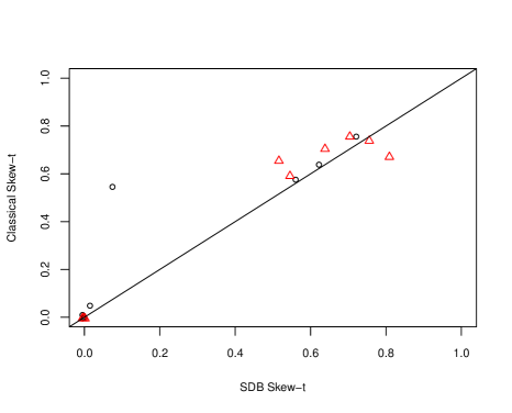
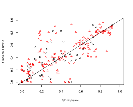
Figure 1: ARI values from model-based clustering analyses of the crabs (left) and AIS (right) data using the EMMIXskew and EMMIXuskew packages, where pairs are represented by circles and triplets by triangles.

In addition to the results in Figure 1, which correspond to SEED=5, the Supplementary Material can be used to easily produce results from other starting values by modifying SEED. As the reader can verify, running the code for SEED=1,...,10 leads to the same message, i.e., neither formulation is superior, but now based on 4,800 cluster analyses. It is noteworthy that the only scenario where the SDB formulation produced better clustering results was constructed by starting the numerical optimization using the true classification labels as the initial values in the numerical search. Of course, assessing a clustering method based on how it does when started at the true classifications is fundamentally flawed because the true classifications are not available in real cluster analyses, assuming that a true classification even exists. Furthermore, such an assessment will lead to an excellent assessment for any method that just does not move from the starts — even a method that simply returns the starting classifications.

A final matter for consideration is the relative computation time for the two formulations. With few exceptions, examples within the literature where the SDB formulation is used for meaningful analysis only consider data with $d\leq 4$; see e. g. Lee and McLachlan (2014, Section 6). It is instructive to consider the ratio of time taken by the SDB formulation to the time taken by the classical formulation for the pairs and triples of the AIS and crabs data. The results of this comparison (Table 1) confirm that the SDB formulation is very much slower than the classical formulation, e.g., taking an average of 7,315 times longer to converge for the three-dimensional crabs data. The R code used to produce the results in Table 1 is available in Supplementary Material.

Table 1: Means and standard deviations for the ratios of user times, from the system.time() function in R, for the SDB formulation to the classical formulation when applied to two- and three-dimensional subsets of the AIS and crabs data.

	Dimension	Mean	Std. Deviation
AIS	2	125.4	160.4
	3	2216.0	2131.9
Crabs	2	307.5	93.5
	3	7315.1	3619.2

5 Conclusion

We have discussed the relative merits of two closely related formulations, each leading to a skewed extension of the multivariate normal and $t$ distribution. For one, we have clarified why the SDB (or “unrestricted”) formulation is not a “simple extension” of the classical (or “restricted”) formulation. We also provide extensive evidence as to why neither formulation is, in general, preferable to the other. Extensive numerical work (4,800 cases in all) was carried out to underline this point in specific reference to clustering applications. We trust it is now clear that the nomenclature “restricted” and “unrestricted” should be avoided in reference to these formulations.

Appendix

Cumulants and Mardia’s coefficients for SDB skew-normal. For the SDB skew-normal, differentiation of $K_{s}(t)=\log M_{s}(t)$ produces

$$\nabla K_{s}(t) = \xi+(\Delta+\Lambda^{2})t+\left[\zeta_{1}(\lambda_{j}t_{j})\lambda_{j}\right]_{j=1}^{d}$$

$$\nabla\nabla^{\top}K_{s}(t) = (\Delta+\Lambda^{2})+\mathrm{diag}(\zeta_{2}(\lambda_{1}t_{1})\lambda_{1}^{2},\dots,\zeta_{2}(\lambda_{d}t_{d})\lambda_{d}^{2}),$$

where $\zeta_{r}(x)$ is the $r$th derivatives of $\zeta_{0}(x)=\log\{2\,\Phi(x)\}$. Evaluation at $t=0$ gives

$$E(Y_{s})=\xi+\sqrt{2/\pi}\>\lambda,\ \ \mathrm{var}(Y_{s})=\Delta+(1-2/\pi)\Lambda^{2}.$$ (6)

Further differentiation and evaluation at $0$ gives the 3rd order cumulant

$$\kappa_{rst}=\left\{\begin{array}[]{ll}\zeta_{3}(0)\,\lambda_{r}^{3}&\mbox{if }r=s=t,\\ 0&\mbox{otherwise},\end{array}\right.$$ (7)

where $\zeta_{3}(0)=b\,(4/\pi-1)=(2/\pi)^{3/2}\>(4-\pi)/2$.

We can now compute the Mardia’s coefficient $\gamma_{1,d}$ of multivariate skewness, recalling that the 3rd order cumulant coincides with the 3rd order central moment. Denote by $\Sigma=(\sigma_{rs})$ the variance matrix in (6) and let $\Sigma^{-1}=(\sigma^{rs})$, $\mu_{j}=b\lambda_{j}$.

From (2.19) of Mardia (1970), write

$$\gamma_{1,d} = \sum_{rst}\sum_{r^{\prime}s^{\prime}t^{\prime}}\kappa_{rst}\kappa_{r^{\prime}s^{\prime}t^{\prime}}\sigma^{rr^{\prime}}\sigma^{ss^{\prime}}\sigma^{tt^{\prime}}=\zeta_{3}(0)^{2}\sum_{u,v}\lambda_{u}^{3}\,\lambda_{v}^{3}\,(\sigma^{uv})^{3}$$ (8)

$$= \left(\frac{4-\pi}{2}\right)^{2}\sum_{u,v}\mu_{u}^{3}\,\mu_{v}^{3}\,(\sigma^{uv})^{3}=\left(\frac{4-\pi}{2}\right)^{2}(\mu^{(3)})^{\top}\Sigma^{(-3)}\mu^{(3)},$$

where $\mu^{(3)}$ is the vector with elements $\mu_{j}^{3}$ and $\Sigma^{(-3)}=\left((\sigma^{uv})^{3}\right)$.

For (8) we do not have an expression of the maximal value. Numerical exploration indicates that the maximal value is $1.98113$, that is, the double value of the classical SN up to the quoted number of digits. This maximal value of $\gamma_{1,d}$ is obtained, irrespectively of $\Delta$, in these four cases:

$$\lambda=h(\pm 1\,\,\pm 1)^{\top},\quad\hbox{when~{}}h\to\infty\,.$$ (9)

Derivation of the 4th order cumulants is similar to (7), leading to

$$\kappa_{rstu}=\left\{\begin{array}[]{ll}\zeta_{4}(0)\,\lambda_{r}^{4}&\mbox{if }r=s=t=u,\\ 0&\mbox{otherwise},\end{array}\right.$$ (10)

where $\zeta_{4}(0)=2\>(\pi-3)\>(2/\pi)^{2}\approx 0.114771$.

From here the Mardia’s coefficient of (excess) kurtosis is

$$\gamma_{2,d} = \sum_{rstu}\kappa_{rstu}\sigma^{rs}\sigma^{tu}$$ (11)

$$= \zeta_{4}(0)\sum_{u}\lambda_{u}^{4}\,(\sigma^{uu})^{2}$$

$$= 2\,(\pi-3)\sum_{u}\mu_{u}^{4}\,\,(\sigma^{uu})^{2}$$

$$= 2\,(\pi-3)(\mu^{(2)})^{\top}(I_{d}\odot\Sigma^{-1})^{2}\mu^{(2)},$$

where $\mu^{(2)}=(\mu_{1}^{2},\dots,\mu_{d}^{2})^{\top}$ and $\odot$ is the Hadamard or component-wise product. A numerical search indicates that the maximal value of $\gamma_{2,d}$ is again achieved, irrespectively of $\Delta$, with $\lambda$ as in (9). The maximal observed value of the coefficient is $1.7383546$, again twice the corresponding value in the classical skew-normal case.

References

- Azzalini and Capitanio (1999) Azzalini, A. and A. Capitanio (1999). Statistical applications of the multivariate skew normal distribution. J. Roy. Stat. Soc., series B 61(3), 579–602.
- Azzalini and Capitanio (2003) Azzalini, A. and A. Capitanio (2003). Distributions generated by perturbation of symmetry with emphasis on a multivariate skew distribution. J. Roy. Stat. Soc., series B 65(2), 367–389.
- Azzalini and Capitanio (2014) Azzalini, A. with the collaboration of A. Capitanio (2014). The Skew-Normal and Related Families. IMS monographs. Cambridge University Press.
- Azzalini and Dalla Valle (1996) Azzalini, A. and A. Dalla Valle (1996). The multivariate skew-normal distribution. Biometrika 83, 715–726.
- Branco and Dey (2001) Branco, M. D. and D. K. Dey (2001). A general class of multivariate skew-elliptical distributions. J. Multivariate Analysis 79, 99–113.
- Campbell and Mahon (1974) Campbell, N. A. and R. J. Mahon (1974). A multivariate study of variation in two species of rock crab of genus leptograpsus. Australian Journal of Zoology 22, 417–425.
- Hubert and Arabie (1985) Hubert, L. and P. Arabie (1985). Comparing partitions. Journal of Classification 2, 193–218.
- Lee and McLachlan (2014) Lee, S. and G. J. McLachlan (2014). Finite mixtures of multivariate skew -distributions: some recent and new results. Statistics and Computing 24, 181–202. Published online 20 October 2012.
- Lee and McLachlan (2013a) Lee, S. X. and G. J. McLachlan (2013a). On mixtures of skew normal and skew -distributions. Advances in Data Analysis and Classification 7, 241–266.
- Lee and McLachlan (2013b) Lee, S. X. and G. J. McLachlan (2013b). EMMIXuskew: An R package for fitting mixtures of multivariate skew distributions via the EM algorithm. Journal of Statistical Software 55(12), 1–22.
- Mardia (1970) Mardia, K. (1970). Measures of multivariate skewness and kurtosis with applications. Biometrika 57, 519–530.
- Peel and McLachlan (2000) Peel, D. and G. J. McLachlan (2000). Robust mixture modelling using the distribution. Statistics and Computing 10, 339–348.
- R Core Team (2014) R Core Team (2014). R: A Language and Environment for Statistical Computing, R Foundation for Statistical Computing,Vienna, Austria.
- Sahu et al. (2003) Sahu, K., D. K. Dey, and M. D. Branco (2003). A new class of multivariate skew distributions with applications to Bayesian regression models. Canad. J. Statist. 31(2), 129–150. Corrigendum: vol. 37 (2009), 301–302.
- Venables & Ripley, (2002) Venables, W. N. & Ripley, B. D. (2002). Modern Applied Statistics with S. New York: Springer, fourth edition.
- Wang et al. (2013) Wang, K., A. Ng, and G. McLachlan. (2013). EMMIXskew: The EM Algorithm and Skew Mixture Distribution. R package version 1.0.1.