Numerical integration for ab initio many-electron self energy calculations within the GW approximation

Abstract

We present a numerical integration scheme for evaluating the convolution of a Green’s function with a screened Coulomb potential on the real axis in the GW approximation of the self energy. Our scheme takes the zero broadening limit in Green’s function first, replaces the numerator of the integrand with a piecewise polynomial approximation, and performs principal value integration on subintervals analytically. We give the error bound of our numerical integration scheme and show by numerical examples that it is more reliable and accurate than the standard quadrature rules such as the composite trapezoidal rule. We also discuss the benefit of using different self energy expressions to perform the numerical convolution at different frequencies.

Key words.

GW, self energy, convolution, numerical integration, trapezoidal rule, principal value integration, COHSEX, XCOR, Dyson’s equation

I Introduction

The computational modeling and simulation of single-electron excitations of molecules and solids including many-electron effects is important for interpreting spectroscopy experiments and predicting excited-state properties of materials. One way to calculate single-particle excitation energies or quasiparticle energies is through Green’s function theory Hedin65 ; Hybertsen86 ; Aryasetiawan98 ; Aulbur00 ; Onida02 . In such a theory, the quasiparticle energies $\varepsilon_{j}$’s and wavefunctions $\phi_{j}(r)$’s are obtained by solving Dyson’s equation Hybertsen86 ; Hedin70 (in atomic units $\hbar=1$, $e=1$, and electron mass $m_{e}=1$)

$$\left[-\frac{1}{2}\nabla^{2}(r)+v_{H}(r)\right]\phi_{j}(r)+\int dr^{\prime}\Sigma(r,r^{\prime};\varepsilon_{j})\phi_{j}(r^{\prime})=\varepsilon_{j}\phi_{j}(r),$$ (1)

where $v_{H}(r)$ is the Hartree potential and $\Sigma(r,r^{\prime};\varepsilon_{j})$ is the energy (or frequency) dependent self energy operator.

The main challenge in solving (1) is the approximation and evaluation of $\Sigma$. One widely used approximation is the $GW$ approximation in which $\Sigma$ is set to the product of a single-particle Green’s function $G$ and a screened Coulomb potential $W$. In the frequency domain, the product is evaluated as a convolution of the time-ordered Fourier transforms of these two functions. Due to the presence of singularities in both functions, the numerical convolution must be carried out with care. This is particularly important for molecules because the poles of $W$ for such systems have more discrete features than those in solids. These poles must be treated properly in the self energy calculation.

There are a number of ways to perform the energy dependent (or full frequency) self energy calculation numerically. One way is use analytic continuation method proposed in Daling91 ; Jin99 ; Rojas95 , another is to perform a contour deformation Kotani02 ; Lebegue03 . A more direct approach is to perform the numerical integration on the real axis, which is the approach we take in this paper. All of these approaches have positive and negative aspects and each approach represents a different way to overcome potential numerical difficulties introduced by the singularity of the integrand.

We will show in this paper that it is important to use a numerical integration scheme that approximates the principal value integral of a singular integrand when the self energy convolution is performed directly on the real axis. We show that failure to do so may lead to significant error in integration over some frequency regions. In this study, we address the singularities in the integration that arise from taking the zero broadening limit in Green’s function only. The approximation to the principal value is obtained by replacing the numerator of the integrand with a piecewise polynomial approximation and performing a principal value integration analytically on the approximate integrand. We show that taking the zero broadening limit improves the accuracy of the numerical integration.

When the spectral representations of $G$ and $W$ are used to derive an expression for $\Sigma$, there are a number of ways to group different terms. These different groupings lead to different expressions. We show that applying the numerical integration scheme proposed in this paper to different expressions may lead to different numerical accuracy. For particular frequency ranges, one expression may be preferred over the other.

II Self energy integration

In the GW approximation, the electron self energy is expressed as $i$ times the product of the time-ordered one-particle Green’s function, denoted by $G(r,r^{\prime};t)$, and a screened Coulomb term, denoted by $W(r,r^{\prime};t)$, in the time domain. Taking a Fourier transform with respect to $t$ yields the frequency representation of the self energy,

$$\Sigma(r,r^{\prime};\omega)=\frac{i}{2\pi}\int_{-\infty}^{\infty}d\omega^{\prime}G(r,r^{\prime};\omega-\omega^{\prime})W(r,r^{\prime},\omega^{\prime})e^{-i\omega^{\prime}\eta},$$ (2)

where $G(r,r^{\prime};\omega)$ and $W(r,r^{\prime};\omega)$ are obtained from Fourier transforms of $G(r,r^{\prime};t)$ and $W(r,r^{\prime};t)$, respectively. Note that the $e^{-i\omega^{\prime}\eta}$ term with a positive infinitesimally small $\eta$ factor is introduced to ensure the proper convergence of the Fourier transform. Such a factor should also appear in the Fourier transforms for $G(r,r^{\prime};\omega)$ and $W(r,r^{\prime};\omega)$ themselves.

In practice, this convolution (2) must be evaluated numerically. The accuracy of the numerical integration can have a significant effect on the quantitative and qualitative behaviors of the approximate solution to Dyson’s equation.

In the frequency domain, Green’s function has the spectral representation

$$G(r,r^{\prime};\omega)=\sum_{j}\frac{\phi_{j}(r)\phi^{*}_{j}(r^{\prime})}{\omega-\varepsilon_{j}+i\eta\text{sgn}(\varepsilon_{j}-\mu)}$$ (3)

where $(\varepsilon_{j},\phi_{j})$, $j=1,2,...$ are quasi-particle eigenvalues (energies) and orbitals enumerated in an increasing energy order. In a computational procedure, they are chosen to be approximate solutions to Dyson’s equation with $\phi_{j}$ evaluated at $\omega=\varepsilon_{j}$ for the self energy $\Sigma$. The first $n_{v}$ eigenpairs are called the valence (or occupied) states, and the remaining ones are referred to as the conduction (or empty) states. The parameter $\mu$ is the chemical potential that satisfies the condition $\varepsilon_{n_{v}}\leq\mu\leq\varepsilon_{n_{v}+1}$.

The screened Coulomb interaction $W$ can be expressed as

$$W(r,r^{\prime};\omega)\equiv\int\epsilon^{-1}(r,r^{\prime\prime};\omega)v(r^{\prime\prime},r^{\prime})dr^{\prime\prime},$$ (4)

where the dielectric function $\epsilon$, defined within the random phase approximation Bohm53 ; GellMann57 , has the form

$$\epsilon(r,r^{\prime};\omega)=\delta(r,r^{\prime})-\int v(r,r^{\prime\prime})\chi_{0}(r^{\prime\prime},r^{\prime};\omega)dr^{\prime\prime},$$

with $v(r,r^{\prime})=1/|r-r^{\prime}|$ being the bare Coulomb potential, and $\chi_{0}(r,r^{\prime};\omega)$ being the time-ordered Fourier transform of the independent particle polarizability function (operator) that describes the linear density response to external potential perturbations. The analytical expression for the non-interacting $\chi_{0}(r,r^{\prime};\omega)$ from a mean-field solution of the system is

$$\begin{split}\chi_{0}(r,r^{\prime};\omega)=&\frac{1}{2}\sum_{i=1}^{n_{v}}\sum_{j>n_{v}}\phi_{i}(r)\phi_{j}^{\ast}(r)\phi^{\ast}_{i}(r^{\prime})\phi_{j}(r^{\prime})\\ &\times\left(\frac{1}{\omega-\Delta\varepsilon_{i,j}+i\eta}-\frac{1}{\omega+\Delta\varepsilon_{i,j}-i\eta}\right),\end{split}$$ (5)

where $\Delta\varepsilon_{i,j}=\varepsilon_{j}-\varepsilon_{i}\geq 0$.

II.1 The analytic structure of the integrand

Because the time-ordered screened Coulomb operator $W$ involves the inverse of the dielectric operator, the analytic structure of the integrand in (2) is not immediately clear. In the following, we examine the finite dimensional approximation of the integrand in (2) in detail, and discuss how the integral (2) can be evaluated numerically.

Let us assume that a proper spatial discretization (e.g., plane-wave expansion) has been used to represent $G$, $W$ and $\Sigma(\omega)$ as $n\times n$ matrices. Using the spectral representation of $G$ and $W$, we can express the integral (2) Hedin65 ; Hybertsen86 ; Hedin70 as

$$\begin{split}\Sigma(\omega)=&-\sum_{j=1}^{n_{v}}\left(\phi_{j}\phi_{j}^{*}\right)\odot W(\omega-\varepsilon_{j})\\ &-\frac{1}{\pi}\sum_{j=1}^{n}(\phi_{j}\phi_{j}^{*})\odot\int^{\infty}_{0}d\omega^{\prime}\frac{(W^{r}(\omega^{\prime})-W^{a}(\omega^{\prime}))/(2i)}{\omega-\varepsilon_{j}-\omega^{\prime}+i\eta},\\ \end{split}$$ (6)

where $W^{r/a}=\left[\epsilon^{r/a}\right]^{-1}V$ are the retarded and advanced screened Coulomb matrix defined in terms of the retarded and advanced dielectric matrices $\epsilon^{r/a}$, which are in turn defined in terms of the retarded and advanced polarizability matrices

$$\begin{split}\chi_{0}^{r/a}(\omega)=&\frac{1}{2}\sum_{i=1}^{n_{v}}\sum_{j=n_{v}+1}^{n}\left(\phi_{i}\odot\overline{\phi_{j}}\right)\left(\phi_{i}\odot\overline{\phi_{j}}\right)^{\ast}\\ &\times\left(\frac{1}{\omega-\Delta\varepsilon_{i,j}\pm i\eta}-\frac{1}{\omega+\Delta\varepsilon_{i,j}\pm i\eta}\right),\end{split}$$ (7)

and the discretized bare Coulomb matrix $V$. We use $\odot$ to denote element-wise multiplication, $\phi_{j}^{\ast}$ to denote the conjugate transpose of a column vector $\phi_{j}$, and $\overline{\phi_{j}}$ to denote the conjugate of $\phi_{j}$. The integral in (6) is performed element-wise. We should also mention that in a practical calculation, the summation over $j$ may be truncated so that the total number of unoccupied states, which we will denote by $n_{c}$, can be less than $n-n_{v}$.

The expression given in (6) is a specific formulation of the self energy. The first term in (6) is the so-called screened exchange (SEX) term and the second term is the Coulomb hole (COH) term. The integrand in the second term of (6) is well behaved in the sense that the integral does not diverge. Such an expression is also physically appealing, especially in the static case ($\omega=0$) Hedin65 .

Without loss of generality, we can write the matrix $\chi_{0}^{r}(\omega)$ as

$$\chi_{0}^{r}(\omega)=M[\Omega(\omega)]^{-1}M^{\ast},$$

where $M$ is an $n\times n_{v}n_{c}$ matrix. Each column of $M$ represents the element-wise product of a discretized $\phi_{i}$ and $\overline{\phi_{j}}$ pair, for $i=1,2,...,n_{v}$, $j=n_{v}+1,n_{v}+2,...,n_{v}+n_{c}$. The $n_{v}n_{c}\times n_{v}n_{c}$ diagonal matrix $[\Omega(\omega)]^{-1}$ has elements

$$\frac{1}{2}\left(\frac{1}{\omega-\Delta\varepsilon_{i,j}+i\eta}-\frac{1}{\omega+\Delta\varepsilon_{i,j}+i\eta}\right)=\frac{\Delta\varepsilon_{i,j}}{(\omega+i\eta)^{2}-\Delta\varepsilon_{i,j}^{2}}.$$ (8)

If we let $V$ be the matrix representation of a discretized unscreened Coulomb operator, we can write $\epsilon^{r}(\omega)$ as

$$\epsilon^{r}(\omega)=I-VM[\Omega(\omega)]^{-1}M^{\ast}.$$ (9)

It follows from the Sherman-Morrison-Woodbury formula Woodbury50 ; Hager89 and some additional algebraic manipulations Liu13 that

$$[\epsilon^{r}(\omega)]^{-1}=I+\sum_{\ell=1}^{n_{v}n_{c}}\frac{1}{2\tau_{\ell}}VMs_{\ell}\left(\frac{1}{\omega-\tau_{\ell}+i\eta}-\frac{1}{\omega+\tau_{\ell}+i\eta}\right)(Ms_{\ell})^{\ast},$$ (10)

where $\tau_{\ell}=\sqrt{\lambda_{\ell}}$ with $\lambda_{\ell}$ being an eigenvalue of the matrix $D^{2}+DM^{\ast}VM$, $D$ is a diagonal matrix with $\Delta\varepsilon_{i,j}$, $i=1,2,...,n_{v}$, $j=n_{v}+1,...,n_{v}+n_{c}$ on its diagonal, and $s_{\ell}$ is the $\ell$th column of $D^{1/2}U$ with $U$ being the matrix that contains all eigenvectors of $D^{2}+D^{1/2}M^{\ast}VMD^{1/2}$. A similar expression can be obtained for $[\epsilon^{a}(\omega)]^{-1}$. Consequently,

$$\begin{split}&(W^{r}(\omega)-W^{a}(\omega))/(2i)\\ =&\sum_{\ell=1}^{n_{v}n_{c}}\frac{1}{2\tau_{\ell}}VMs_{\ell}\left[\frac{\eta}{(\omega+\tau_{\ell})^{2}+\eta^{2}}-\frac{\eta}{(\omega-\tau_{\ell})^{2}+\eta^{2}}\right](VMs_{\ell})^{\ast}.\end{split}$$ (11)

The expression given by (11) indicates that all matrix elements of the integrand of the integration in (6) (in any basis) have the same analytic structure.

In principle, if $\tau_{\ell}$’s are known, the integration in (6) can be evaluated analytically for all $\omega$. In the limit of $\eta\rightarrow 0$, $\eta/[(\omega^{\prime}\pm\tau_{\ell})^{2}+\eta^{2}]$ becomes a $\delta$-function centered at $\omega^{\prime}=\mp\tau_{\ell}$. Because $\tau_{\ell}=\sqrt{\lambda_{\ell}}$ is nonnegative, the COH term in (6) simplifies to

$$I_{\text{COH}}=\frac{1}{\pi}\sum_{j=1}^{n}\left(\phi_{j}\phi_{j}^{\ast}\right)\odot\left[\sum_{\ell=1}^{n_{v}n_{c}}\frac{1}{2\tau_{\ell}}\frac{VMs_{\ell}(VMs_{\ell})^{\ast}}{\omega-\varepsilon_{j}-\tau_{\ell}}\right].$$ (12)

However, obtaining $\tau_{\ell}$ requires computing all eigenvalues of an $n_{v}n_{c}\times n_{v}n_{c}$ matrix, a task that requires $\mathcal{O}(n^{6})$ operations even though $\Sigma$ and $\epsilon^{r/a}$ are $n\times n$ matrices Casida95 ; Tiago06 ; Lischner12 . This can be costly for large systems that contain many atoms. An alternative way to evaluate the integral in (6) numerically is to evaluate the integrand at multiple values of $\omega^{\prime}$ and use an appropriate quadrature rule to sum up these function evaluations. In this approach, the $\epsilon^{r/a}(\omega^{\prime})$ matrices must be evaluated at a number of frequencies. Each evaluation is expensive, because it requires computing $\chi_{0}^{r/a}(\omega^{\prime})$ for each $\omega^{\prime}$, multiplying $\chi_{0}^{r/a}(\omega^{\prime})$ with $V$ and inverting the product. The complexity of the evaluation is $\mathcal{O}(n^{4})$ for each $\omega^{\prime}$, where $n$ scales linearly with the number of atoms in the system. Therefore, we would like to minimize the number of such evaluations as much as possible without sacrificing the accuracy of the integration.

II.2 Separating the low and high frequency regions

Let $S_{\eta}(\omega^{\prime})=(W^{r}(\omega^{\prime})-W^{a}(\omega^{\prime}))/(2i)$. In frequency regions where the poles of $S_{\eta}(\omega^{\prime})$ are near $\omega-\varepsilon_{j}$, the direct numerical integration of (6) may be difficult due to the presence of singularities in the integrand. As a result, more quadrature points need to be placed near the poles of $S_{\eta}(\omega^{\prime})$. However, in the tail regions of $1/(\omega-\varepsilon_{j}-\omega^{\prime}+i\eta)$, that are far away from these poles, the Lorentzians in $S_{\eta}(\omega^{\prime})$ should decay to zero rapidly. Fewer quadrature points are thus needed to approximate the COH term in that region by a weighted sum. In particular, we can use a Gauss quadrature rule, i.e.

$$\int_{a}^{b}d\omega^{\prime}\frac{S_{\eta}(\omega^{\prime})}{\omega-\varepsilon_{j}-\omega^{\prime}+i\eta}\approx\sum_{i=1}^{P}\frac{S_{\eta}(\omega^{\prime}_{i})}{\omega-\varepsilon_{j}-\omega^{\prime}_{i}+i\eta}\nu_{i},$$ (13)

where $\omega^{\prime}_{i}$ are quadrature points at which the integrand is evaluated and $\nu_{i}$ are the properly chosen weights. Typically, ten or twenty quadrature points are sufficient to produce a highly accurate integral.

For a given $\omega$, we can apply (13) to the high frequency interval $[\xi,\infty)$ where $\xi=\max(\omega-\varepsilon_{1},\max_{\ell}\tau_{\ell})+\zeta$, for some modest constant $\zeta\geq 0$. Here $\tau_{\ell},~{}\ell=1,2,\cdots,n_{v}n_{c}$ are the position of poles of $S_{\eta}(\omega^{\prime})$ for $\omega^{\prime}\geq 0$ as shown in (11). If we view the matrix $DM^{\ast}VM$ as a small perturbation to the diagonal matrix $D^{2}$ whose diagonal elements are $(\Delta\varepsilon_{i,j})^{2}$, the poles of $S_{\eta}(\omega^{\prime})$ should not be too far away from $\pm\Delta\varepsilon_{i,j}$. Hence we can simply estimate $\max_{\ell}\tau_{\ell}$ by $\varepsilon_{\max}-\varepsilon_{1}$, where $\max=n_{v}+n_{c}$. Because the $\omega$’s of interest are often within $[\varepsilon_{1},\varepsilon_{\max}]$, choosing $\xi=\varepsilon_{\max}-\varepsilon_{1}+\zeta$ as the starting point of the high frequency region is not unreasonable. Below this region, i.e., within the interval $(0,\varepsilon_{\max}-\varepsilon_{1})$, a different numerical integration strategy that accounts for the singular nature of the integrand must be used. We will describe that strategy in the next section.

To confirm the above observation, we plot both the poles of a typical matrix element of the $\epsilon^{r}(\omega)$ and $S_{\eta}(\omega)$ associated with a SiH4 molecule in Figure 1. Our calculation is performed using KSSOLV Yang09 , which is a MATLAB toolbox for solving the Kohn-Sham problem. The plane-wave expansion is used for discretizing $\epsilon^{r}(\omega)$ and $S_{\eta}(\omega)$. $(\varepsilon_{j},\phi_{j})$’s are taken to be the Kohn-Sham DFT eigenpairs. We will use $\varepsilon_{LUMO}$ and $\varepsilon_{HOMO}$ to denote the lowest unoccupied (empty) and the highest occupied Kohn-Sham single-particle eigenvalues below, i.e. $\varepsilon_{LUMO}=\varepsilon_{n_{v}+1}$ and $\varepsilon_{HOMO}=\varepsilon_{n_{v}}$.

Figure 1 shows that poles of $\epsilon^{r}(\omega)$, which are at $\Delta\varepsilon_{i,j}$, and those of $S_{\eta}(\omega)$, which are at $\tau_{\ell}$, match up pretty well. In particular, they are both in the domain $[\min\Delta\varepsilon_{i,j},\max\Delta\varepsilon_{i,j}]=[\varepsilon_{LUMO}-\varepsilon_{HOMO},\varepsilon_{\max}-\varepsilon_{1}]=[3.2,20.9]$ eV. Outside of this region, the magnitude of $S_{\eta}(\omega)$ decreases rapidly to zero.

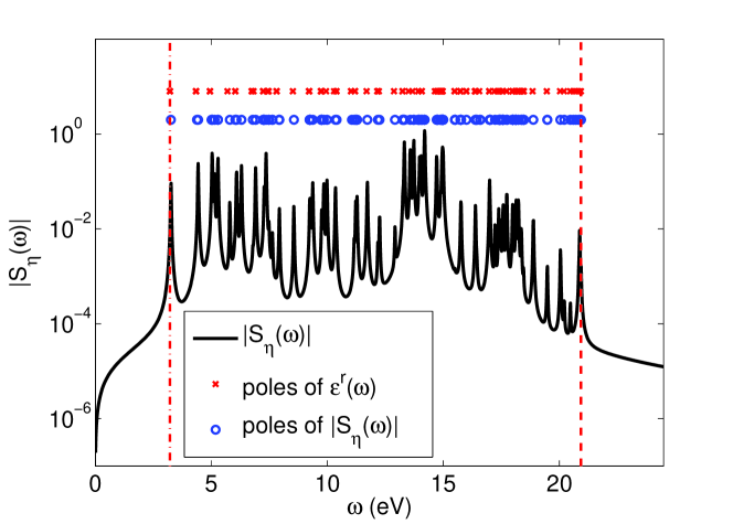
Figure 1: The diagonal element of $|S_{\eta}(\omega)|$ of SiH4, associated with $G=G^{\prime}=[2~{}0~{}0]$, is shown as the black curve. $G$, $G^{\prime}$ are in units of the reciprocal basis $2\pi/a_{0}$ of the supercell containing the molecule with $a_{0}=10$ Bohr. The top of the figure shows the positions of the poles associated with the corresponding entry in the $\epsilon^{r}(\omega)$ matrix (the red crosses), as well as the positions of poles of $|S_{\eta}(\omega)|$ (the blue circles).

II.3 Quadrature for the low frequency region

The fundamental problem we need to solve in order to evaluate (6) efficiently and accurately is to properly evaluate an integral of the form

$$I_{\eta}(\gamma)=\int_{0}^{\infty}\frac{f(\omega^{\prime})}{\omega^{\prime}-\gamma+i\eta}d\omega^{\prime}$$ (14)

for $\gamma>0$, where $f(\omega^{\prime})$ contains a linear combination of a number of Lorentzians centered at $\tau_{\ell}$’s, which we do not know in advance.

Taking the $\eta\rightarrow 0$ limit in the denominator of the integrand reduces the integral to

$$I_{\eta}(\gamma)=-i\pi f(\gamma)+\mbox{PV}\int_{0}^{\infty}\frac{f(\omega^{\prime})}{\omega^{\prime}-\gamma}d\omega^{\prime},$$ (15)

where PV denotes the principal value.

Hence, we shall now focus on the numerical evaluation of the principal value integral in (15).

A simple quadrature rule for integrating $f(\omega^{\prime})/(\omega^{\prime}-\gamma)$ numerically on the interval $[a,b]$ is the composite trapezoidal rule. If we let

$$\omega^{\prime}_{i}=a+(i-1)h,\quad i=1,\ldots,N,$$

where $h=(b-a)/(N-1)$, the trapezoidal rule gives the following approximation:

$$\int^{b}_{a}\frac{f(\omega^{\prime})}{\omega^{\prime}-\gamma}d\omega^{\prime}=\sum_{i=1}^{N-1}\frac{1}{2}\left(\frac{1}{\omega^{\prime}_{i}-\gamma}f(\omega^{\prime}_{i})+\frac{1}{\omega^{\prime}_{i+1}-\gamma}f(\omega^{\prime}_{i+1})\right)h.$$ (16)

However, the trapezoidal rule generally does not converge to the principal value of integral in (15), even if $h$ is chosen to be very small. To see this, let us assume that that $\gamma\in(\omega^{\prime}_{I},\omega^{\prime}_{I+1})$, for some $1\leq I\leq N-1$. (If $\gamma=\omega_{i}^{\prime}$ for some $i$, we move $\omega_{i}^{\prime}$ slightly away from $\gamma$ to avoid floating point overflow.) That is, we assume that $\gamma$ can be close to an integration point $\omega^{\prime}_{I}$, but never be exactly equal to $\omega^{\prime}_{I}$.

If $\gamma-\omega^{\prime}_{I}=\alpha h$ for some $0<\alpha\ll 1$, it follows that the term

$$\left\lvert\frac{f(\omega^{\prime}_{I})h}{\omega^{\prime}_{I}-\gamma}\right\rvert=\left\lvert\frac{f(\omega^{\prime}_{I})}{\alpha}\right\rvert$$ (17)

in the summation will dominate over other terms in Eq. (16) if $\alpha\ll\left\lvert f(\omega^{\prime}_{I})\right\rvert$. As $\alpha\to 0$, the right hand side of (16) behaves like $1/\alpha$, and it rapidly approaches $\infty$ independent of $h$. No other term with an opposite sign can offset this large spike. This undesirable behavior can lead to sharp artificial peaks in the self energy at some $\omega$ values, as we will show in the next section. This issue cannot be addressed by simply using a higher order numerical integration scheme (such as Simpson’s rule) that does not preserve the principal value of the integral.

One way to mitigate the singularity issue is to resort to an alternative numerical integration scheme that replaces $f(\omega^{\prime})$, instead of the entire integrand, with an approximation, and perform a principal value integration of the approximated integrand analytically on each interval $[\omega^{\prime}_{i},\omega^{\prime}_{i+1}]$. The simplest approximation of $f(\omega^{\prime})$ is the piecewise constant approximation $f(\omega^{\prime})\approx[f(\omega^{\prime}_{i})+f(\omega^{\prime}_{i+1})]/2$ for $\omega^{\prime}\in[\omega^{\prime}_{i},\omega^{\prime}_{i+1}]$. Such an approximation leads to the following quadrature rule:

$$\text{PV}\int^{b}_{a}\frac{f(\omega^{\prime})}{\omega^{\prime}-\gamma}d\omega^{\prime}\approx\sum_{i}\frac{1}{2}\left[f(\omega^{\prime}_{i})+f(\omega^{\prime}_{i+1})\right]\text{log}\left|\frac{\omega^{\prime}_{i+1}-\gamma}{\omega^{\prime}_{i}-\gamma}\right|.$$ (18)

A more accurate approximation is a piecewise linear approximation of $f(\omega^{\prime})$, which leads to the following quadrature rule:

$$\begin{split}\text{PV}\int^{b}_{a}\frac{f(\omega^{\prime})}{\omega^{\prime}-\gamma}d\omega^{\prime}\approx&\sum_{i}\left[f(\omega^{\prime}_{i+1})-f(\omega^{\prime}_{i})\right.\\ &\left.+\left(f(\omega^{\prime}_{i})+\frac{f(\omega^{\prime}_{i+1})-f(\omega^{\prime}_{i})}{\omega^{\prime}_{i+1}-\omega^{\prime}_{i}}(\gamma-\omega^{\prime}_{i})\right)\text{log}\left|\frac{\omega^{\prime}_{i+1}-\gamma}{\omega^{\prime}_{i}-\gamma}\right|\right].\end{split}$$ (19)

If we denote the absolute error made in (18) and (19) by $E_{c}$ and $E_{l}$ respectively, it is not difficult to show Liu13 that

$$E_{c} \leq C_{c}h||f^{\prime}||_{\infty}\left(1+\left\lvert\log h\right\rvert+\left\lvert\log\alpha\right\rvert+\left\lvert\log(1-\alpha)\right\rvert\right),$$ (20)

$$E_{l} \leq C_{l}h^{2}||f^{\prime\prime}||_{\infty}(1+\left\lvert\log h\right\rvert),$$ (21)

for some constants $C_{c}$ and $C_{l}$ that are independent of $h$. These error bounds indicate that the accuracy of the quadrature should improve as we decrease $h$.

In (18) consider $\gamma-\omega^{\prime}_{I}=\alpha h$ with $0<\alpha\ll 1$ and the term

$$\begin{split}&\frac{1}{2}\left(f(\omega^{\prime}_{I-1})+f(\omega^{\prime}_{I})\right)\log\left\lvert\omega^{\prime}_{I}-\gamma\right\rvert-\frac{1}{2}\left(f(\omega^{\prime}_{I})+f(\omega^{\prime}_{I+1})\right)\log\left\lvert\omega^{\prime}_{I}-\gamma\right\rvert\\ &=\frac{1}{2}\left(f(\omega^{\prime}_{I-1})-f(\omega^{\prime}_{I+1})\right)\log(\alpha h).\end{split}$$ (22)

This term becomes the dominating term if $\alpha\ll\exp\{-\frac{1}{\left\lvert f(\omega^{\prime}_{I-1})-f(\omega^{\prime}_{I+1})\right\rvert}\}/h$.

Note that $\left\lvert f(\omega^{\prime}_{I-1})-f(\omega^{\prime}_{I+1})\right\rvert\sim O(h)$, and that $\lim_{h\to 0}e^{-C/h}/h=0$. Thus, for a given $\alpha$, we can always find an $h$ small enough such that (22) does not become the dominating term. As a result, even if we replace $f(\omega^{\prime})$ by a piecewise constant, the corresponding quadrature is more stable than the standard trapezoid rule. Using the piecewise linear approximation further improves the accuracy of the numerical integration without incurring additional function evaluation cost.

An alternative way to overcome the difficulty with the singularity is to keep the parameter $\eta$ finite in the denominator of the integrand in (14). In this case, we can also replace $f(\omega^{\prime})$ with a piecewise polynomial (or spline) approximation and integrate the approximate integrand analytically on each interval. For example, if we approximate $f(\omega^{\prime})$ by a piecewise linear function, the quadrature rule, which is used in Shishkin06 , becomes

$$\begin{split}&\int^{b}_{a}\frac{f(\omega^{\prime})}{\omega^{\prime}-\gamma+i\eta}d\omega^{\prime}\\ =&\sum_{i}\left[\frac{f(\omega^{\prime}_{i})}{\omega^{\prime}_{i}-\omega^{\prime}_{i-1}}\int^{\omega^{\prime}_{i}}_{\omega^{\prime}_{i-1}}\frac{\omega^{\prime}-\omega^{\prime}_{i-1}}{\omega^{\prime}-\gamma+i\eta}d\omega^{\prime}+\frac{f(\omega^{\prime}_{i+1})}{\omega^{\prime}_{i}-\omega^{\prime}_{i+1}}\int^{\omega^{\prime}_{i+1}}_{\omega^{\prime}_{i}}\frac{\omega^{\prime}-\omega^{\prime}_{i+1}}{\omega^{\prime}-\gamma+i\eta}d\omega^{\prime}\right].\end{split}$$ (23)

The integrals within the square brackets above can be evaluated analytically. To simplify our discussion, we do not give the analytical expression here, which is slightly more complicated than the $\log$ function that appears in (19).

Our numerical examples in the next section show that the quadrature rule based on (23) is not as accurate as the one based on (15) and (19). The effect of the broadening parameter is visible near at least some frequencies.

II.4 Different explicit forms: full-frequency COHSEX vs. XCOR

We should mention that applying the numerical integration scheme to the full-frequency COH term in (6) and evaluating the SEX term directly by computing $W(\omega-\varepsilon_{j})$ according to (4) can create a potential numerical issue. To see this, we express $W(\omega-\varepsilon_{j})$ in terms of its spectral representation

$$W(\omega-\varepsilon_{j})=V-\frac{1}{\pi}\int_{0}^{\infty}d\omega^{\prime}S_{\eta}(\omega^{\prime})\left[\frac{1}{\omega-\varepsilon_{j}-\omega^{\prime}+i\eta}-\frac{1}{\omega-\varepsilon_{j}+\omega^{\prime}-i\eta}\right].$$ (24)

Under this representation, the SEX term can be seen to contain the component

$$\frac{1}{\pi}\sum_{j=1}^{n_{v}}(\phi_{j}\phi_{j}^{\ast})\odot\int_{0}^{\infty}d\omega^{\prime}\frac{S_{\eta}(\omega^{\prime})}{\omega-\varepsilon_{j}-\omega^{\prime}+i\eta},$$ (25)

which cancels with the summation over the occupied states in the COH term. After the cancellation, what is left can be written as

$$\begin{split}\Sigma(\omega)=&-\sum_{j=1}^{n_{v}}(\phi_{j}\phi_{j}^{\ast})\odot V-\frac{1}{\pi}\sum_{j=1}^{n_{v}}(\phi_{j}\phi_{j}^{\ast})\odot\int_{0}^{\infty}d\omega^{\prime}\frac{S_{\eta}(\omega^{\prime})}{\omega-\varepsilon_{j}+\omega^{\prime}-i\eta}\\ &-\frac{1}{\pi}\sum_{j=n_{v}+1}^{n}(\phi_{j}\phi_{j}^{\ast})\odot\int_{0}^{\infty}d\omega^{\prime}\frac{S_{\eta}(\omega^{\prime})}{\omega-\varepsilon_{j}-\omega^{\prime}+i\eta}.\end{split}$$ (26)

We call this expression for the self energy the XCOR expression because the first term of the expression is exactly the exchange (X) term, and what is left over can be viewed as the correlation (COR) term.

The XCOR and COHSEX expressions are mathematically equivalent. They correspond to different ways of grouping different terms when spectral representations of $G$ and $W$ are substituted into (2). However, because the denominator of the first integrand in (26) is slightly different from that in (6), and the single-particle states over which the summations are performed are also different in these expressions, numerical integration can give different results. Depending on the $\omega$ value of interest, it may be more advantageous to numerically integrate one expression than the other.

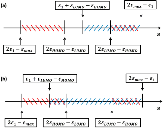
Figure 2: The regions of $\omega$ in which the SFC is violated for the full-frequency COHSEX (blue slashes) and XCOR (red backslashes) expressions. In (a), we assume $2\varepsilon_{HOMO}-\varepsilon_{LUMO}<\varepsilon_{1}+\varepsilon_{LUMO}-\varepsilon_{HOMO}$. In (b), we assume $2\varepsilon_{HOMO}-\varepsilon_{LUMO}>\varepsilon_{1}+\varepsilon_{LUMO}-\varepsilon_{HOMO}$.

More precisely, we should choose an expression in which the centers of the Lorentzians in the numerator ($S_{\eta}(\omega^{\prime})$) of the integrand do not lie in a region that contains $\omega^{\prime}$ values that make the denominator nearly zero. We will refer to this criterion as the singularity-free criterion (SFC).

For simplicity, from now on, we use the following notations for different groups of indexes. Let $I_{occ}=\{1,2,\cdots,n_{v}\}$, $I_{emp}=\{n_{v}+1,n_{v}+2,\cdots,\max\}$, $I_{all}=\{1,2,\cdots,\max\}$, and $I_{\ell}=\{1,2,\cdots,n_{v}n_{c}\}$. Because the centers of the Lorentzians in the numerators, denoted by $\tau_{\ell}$’s ($\ell\in I_{\ell}$), are the positions of the poles of $\left[\epsilon^{r/a}\right]^{-1}$, which roughly lie in the region $[\varepsilon_{LUMO}-\varepsilon_{HOMO},\varepsilon_{\max}-\varepsilon_{1}]$ as we explained in Section II.2, we can estimate regions of $\omega$ in which the SFC is violated for both the COHSEX and the XCOR expressions. The integrand in the COHSEX expression (6) has poles near $\omega-\varepsilon_{j}(j\in I_{all})$. Thus, the SFC is violated when $\omega\approx\varepsilon_{j}+\tau_{\ell}$. Hence, the region in which SFC is violated can be estimated by

$$\left[\min_{j\in I_{all}\atop\ell\in I_{\ell}}\{\varepsilon_{j}+\tau_{\ell}\},\max_{j\in I_{all}\atop\ell\in I_{\ell}}\{\varepsilon_{j}+\tau_{\ell}\}\right]\approx\left[\varepsilon_{1}+\varepsilon_{LUMO}-\varepsilon_{HOMO},2\varepsilon_{\max}-\varepsilon_{1}\right].$$ (27)

This region is marked by blue slashes in Figure 2. A similar analysis shows that the integrand in (26) has singularities near $\omega\approx\varepsilon_{j}-\tau_{\ell}(j\in I_{occ})$ due to the second term in (26) and near $\omega\approx\varepsilon_{j}+\tau_{\ell}(j\in I_{emp})$ due to the third term. Hence, the regions in which the SFC is violated for the XCOR expression can be estimated by

$$\begin{split}&\left[\min_{j\in I_{occ}\atop\ell\in I_{\ell}}\{\varepsilon_{j}-\tau_{\ell}\},\max_{j\in I_{occ}\atop\ell\in I_{\ell}}\{\varepsilon_{j}-\tau_{\ell}\}\right]\bigcup\left[\min_{j\in I_{emp}\atop\ell\in I_{\ell}}\{\varepsilon_{j}+\tau_{\ell}\},\max_{j\in I_{emp}\atop\ell\in I_{\ell}}\{\varepsilon_{j}+\tau_{\ell}\}\right]\\ =&\left[\varepsilon_{1}-\max\tau_{\ell},\varepsilon_{HOMO}-\min\tau_{\ell}\right]\bigcup\left[\varepsilon_{LUMO}+\min\tau_{\ell},\varepsilon_{\max}+\max\tau_{\ell}\right]\\ \approx&\left[2\varepsilon_{1}-\varepsilon_{\max},2\varepsilon_{HOMO}-\varepsilon_{LUMO}\right]\bigcup\left[2\varepsilon_{LUMO}-\varepsilon_{HOMO},2\varepsilon_{\max}-\varepsilon_{1}\right].\end{split}$$ (28)

These regions are marked by the red backslash symbols in Figure 2.

Since $\varepsilon_{1}+\varepsilon_{LUMO}-\varepsilon_{HOMO}$ is not always greater (or less) than $2\varepsilon_{HOMO}-\varepsilon_{LUMO}$, two scenarios must be considered. They are shown in Figure 2 (a) and (b) seperately. Clearly, Figure 2 shows that the XCOR expression is always better than the COHSEX expression in the frequency region $[2\varepsilon_{HOMO}-\varepsilon_{LUMO}$, $2\varepsilon_{LUMO}-\varepsilon_{HOMO}]$, because in this region the SFC always holds for the XCOR expression but not necessarily for COHSEX. Thus, even the trapezoidal rule may work reasonably well for the XCOR expression. The COHSEX expression is always preferred in $\left[2\varepsilon_{1}-\varepsilon_{\max},\varepsilon_{1}+\varepsilon_{LUMO}-\varepsilon_{HOMO}\right]$. We can also see that in $\left[2\varepsilon_{LUMO}-\varepsilon_{HOMO},2\varepsilon_{\max}-\varepsilon_{1}\right],$ the SFC is violated for both the COHSEX and XCOR expressions. Therefore, in this region (where the blue slashes intersect with the red blackslashes in Figure 2), the use of the trapezoidal rule is likely to result in large errors regardless whether the COHSEX or XCOR expression is used.

III Numerical example

In this section, we demonstrate the advantage of using the principal value integration based on quadrature rule such as (19) to perform the self energy integration. We will first illustrate this point by using a simple model test problem in section III.1 of which we know the exact solution. We then show the effects of using different numerical integration schemes on the full-frequency COHSEX and XCOR expressions of the self energy for a small molecule. These tests are performed by modifying and running the BerkeleyGW software package Deslippe12 .

III.1 Model test problem

In the simple model test problem, we choose $f(\omega^{\prime})$ in (14) to be a single Lorentzian centered at 0, i.e., we let

$$f(\omega^{\prime})=\frac{\eta}{\omega^{\prime 2}+\eta^{2}},$$

with $\eta$ set to 0.1, and evaluate

$$I(\gamma)=\int^{10}_{-10}\frac{f(\omega^{\prime})}{\omega^{\prime}-\gamma}d\omega^{\prime},$$ (29)

for a set of $\gamma$ values within $[-1,1]$. The analytical solution to this integration problem is

$$\begin{split}I(\gamma)=&-\frac{1}{2(\gamma^{2}+\eta^{2})}\left[\eta\log\left|\frac{(10+\gamma)^{2}+\eta^{2}}{(-10+\gamma)^{2}+\eta^{2}}\right|\right.\\ &\left.+2\gamma\left(\arctan\left(\frac{10+\gamma}{\eta}\right)-\arctan\left(\frac{-10+\gamma}{\eta}\right)\right)\right].\end{split}$$

Hence, we can compute the errors associated with different numerical integration schemes.

In all our numerical integration schemes, we choose the integration step size to be $h=\eta=0.1$.

In Figure 3, the exact $I(\gamma)$, the approximation obtained from different numerical integration schemes ((16), (18) and (19)) and their corresponding relative errors are shown. We can clearly see that the relative errors associated with the trapezoidal rule can be two orders of magnitude larger than those associated with the alternative quadrature rules (18) and (19).

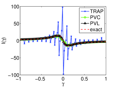
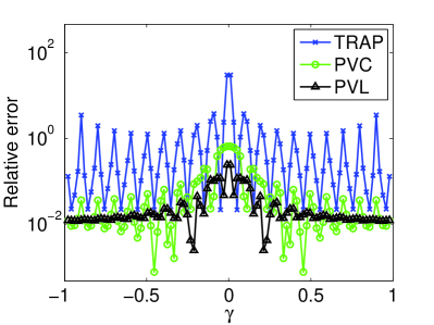
Figure 3: The results produced by the trapezoidal rule (TRAP) applied directly to (29) and alternative quadrature rules that perform a principal value integration analytically after $f(\omega^{\prime})$ is approximated by a piecewise constant function (PVC) and a piecewise linear function (PVL). Left: the analytic (“exact”) integral $I(\gamma)$ and the numerical approximations of $I(\gamma)$. Right: the relative errors.

We observe that the largest error occurs near (but not at) $\gamma=0$ where the Lorentzian has a relatively large value, and the nearest two integration points are not symmetric with respect to $\gamma$. This observation is consistent with the analysis in section II.3.

III.2 The self energy of methane

We now show how different integration schemes perform for the self energy calculation of a methane molecule. We implemented (16), (18), (19), and (23) in the BerkeleyGW software Deslippe12 . We applied these integration schemes to both the full-frequency COHSEX and XCOR self energy expressions. The abbreviations for these schemes and the corresponding legends we use for plotting are listed in Table 1.

Label	Integration scheme	Legend for plotting
COHSEX-TRAP	Trapezoidal rule applied to the full-frequency COHSEX expression	cyan line (square)
COHSEX-PVC	Replace the numerator of the COH term by a piecewise constant approximation and perform principal value integration analytically (18)	black dash line (cross)
COHSEX-PVL	Replace the numerator of the COH term by a piecewise linear approximation and perform principal value integration analytically (19)	blue line (circle)
XCOR-TRAP	Trapezoidal rule applied to the XCOR expression	green line (diamond)
XCOR-PVC	Replace the numerator of the COR term by a piecewise constant approximation and perform principal value integration analytically (18)	blue dash line (circle)
XCOR-PVL	Replace the numerator of the COR term by a piecewise linear approximation and perform principal value integration analytically (19)	black line (cross)

Table 1: Labels for different numerical integration schemes tested.

We compare our results with an analytical integration scheme based on (12) Casida95 ; Tiago06 ; Lischner12 . Because the analytical integration scheme takes the $\eta\rightarrow 0$ limit in both the numerator and denominator of the integrand, and introduces broadening later on for plotting, our numerical integration results will never be exactly the same as analytical results. However, a numerically accurate integration scheme should be close to the analytical result, and should not exhibit unexpected features (e.g., peaks) not present in the analytical results.

We use the plane-wave density-functional theory (DFT) program Quantum Espresso Giannozzi09 to compute the ground-state Kohn-Sham eigenvalues $\varepsilon_{j}$ and wavefunctions $\phi_{j}$ of a methane molecule placed in a supercell of size $16\times 16\times 16~{}\text{Bohr}^{3}$. The Perdew-Burke-Ernzherhof (PBE) approximation Perdew96 to the exchange-correlation functional, and Troullier-Martins norm-conserving pseudopotentials TroullierM91 are used in the DFT calculation. The plane-wave kinetic energy cutoff used in the calculation is 90 Ry. The self energy is approximated by the so-called $G_{0}W_{0}$ scheme in which both Green’s function (3) and the screened Coulomb term (4) are constructed from the ground-state Kohn-Sham eigenpairs. The polarizability, dielectric function and self energy are all calculated using the BerkeleyGW software package Deslippe12 . In the polarizability calculation, we truncate the empty states summation and use only $n_{c}=52$ conduction (empty) states. The number of valence (occupied) states is $n_{v}=4$. We employ a 5.0 Ry dielectric matrix truncation cutoff and truncate the bare Coulomb in the real space beyond the 10 Bohr radius. It should be pointed out that this is not a converged calculation considering the small number of empty states and $(G,G^{\prime})$ pairs determined by the dielectric matrix truncation. The purpose of this calculation is merely to analyze and compare different numerical integration schemes.

The broadening parameter $\eta$ is set to 0.1 eV. As we explained in the previous section, the numerical integration of (2) is performed separately on two regions. In the low frequency region $[0.0,30.0]$ eV, the integration is performed by using a uniform grid with 0.1 eV spacing between the grid points. This is the region where all of the poles of the $S_{\eta}(\omega^{\prime})$ lie. A coarser grid is chosen for the integration performed on $[30.0,120.0]$ eV because the integrand varies slowly with respect to $\omega^{\prime}$ in this region and its magnitude is relatively small. Beyond $120.0$ eV, the integrand is negligibly small so that the integral of the tail can be ignored.

In Figure 4, we plot the real part of the HOMO component of $\Sigma(\omega):\langle\phi_{4}|\Sigma(\omega)|\phi_{4}\rangle$ where the vacuum correction $-0.254$ eV is included, for a number of $\omega$ values between $-30$ eV and $10$ eV. Four different integration schemes are used to generate the plot. As a reference, we also show the self energy values computed from the analytic expression (12), which we consider to be “exact”. This figure shows that the use of principal value integration is the key to maintaining the accuracy of the numerical integration scheme regardless whether the COHSEX or XCOR expression of the self energy is used. If we simply apply the trapezoidal rule to integrate the COHSEX expression, large errors are observed in the frequency region $[$-8, 10$]$ eV. Similarly, large error is observed in the $[$-30, -20$]$ eV region when the trapezoidal rule is applied to the XCOR expression. This observation is consistent with the analysis given in section II.4. Using the parameters given in Table 2, we can estimate the region of $\omega$ in which the SFC is violated for the COHSEX expression to be $\left[\varepsilon_{1}+\varepsilon_{LUMO}-\varepsilon_{HOMO},2\varepsilon_{\max}-\varepsilon_{1}\right]=[$-8.1, 37.0$]$ eV. This interval contains the interval $[$-8, 10$]$ eV in which large errors are observed for integrating the COHSEX expression with the trapezoidal rule. Similarly, the estimated region in which the SFC is violated for the XCOR expression is $[-43.7,-17.9]\cup[8.2,37.0]$ eV. This is also consistent with our observation.

$\varepsilon_{1}$	$\varepsilon_{HOMO}$	$\varepsilon_{LUMO}$	$\varepsilon_{\max}$	$\varepsilon_{LUMO}-\varepsilon_{HOMO}$	$\varepsilon_{\max}-\varepsilon_{1}$
-16.8	-9.2	-0.5	10.1	$8.7$	$26.9$

Table 2: The ground-state Kohn-Sham eigenvalues $\varepsilon_{j}$ (in unit eV) for methane obtained from Quantum Espresso Giannozzi09 .

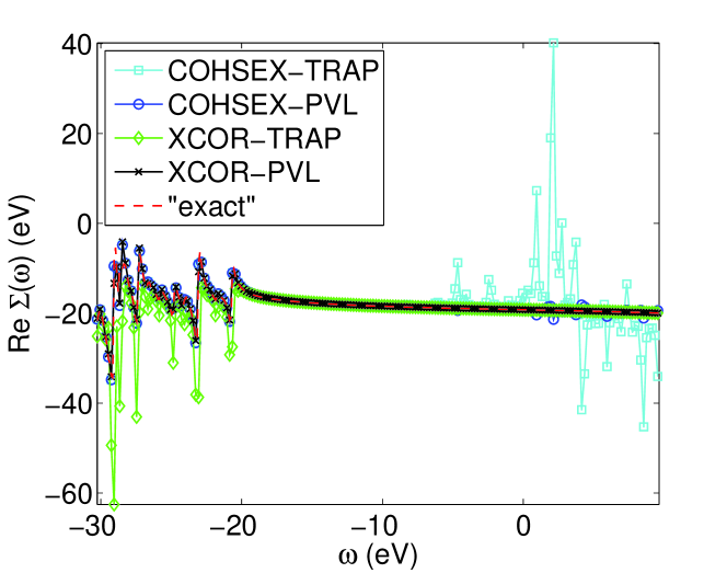
Figure 4: The real part of $\langle\phi_{4}|\Sigma(\omega)|\phi_{4}\rangle$ for a methane molecule computed by four different numerical integration schemes.

In Figure 5, we zoom in Figure 4 and observe that the use of principal value integration indeed dramatically reduces the amount of numerical integration error for both the COHSEX and XCOR expression. For example, for $\omega\in[-25,-23.5]$ eV, COHSEX is the preferred expression to integrate because the COH terms does not have any pole in the region of integration. For $\omega\in[-6,4]$ eV, XCOR is clearly the preferred expression to integrate. However, even if the preferred expression is not used for the integration, the accuracy of the principal value integration improves when a better approximation of the numerator (e.g., piecewise linear) is used. The use of higher order approximation of the numerator also allows us to use a larger $h$ and fewer function evaluations.

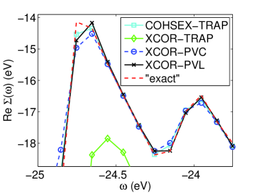
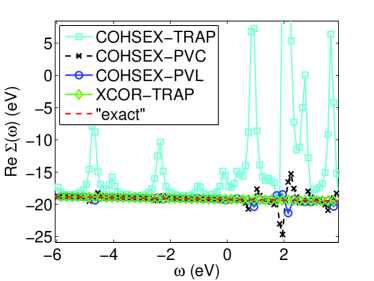
Figure 5: The computed real part of $\langle\phi_{4}|\Sigma(\omega)|\phi_{4}\rangle$ for a methane molecule where $\omega\in[-25,-23.5]\cup[-6,4]$ eV.

In Figure 6, we demonstrate the benefit of taking the $\eta\rightarrow 0$ limit in the denominator of (14) first before performing the principal value integration. Without taking this limit first, the principal value integration based on  (23) produces much larger error for both the COHSEX and XCOR expressions in different frequency regions.

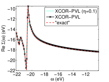
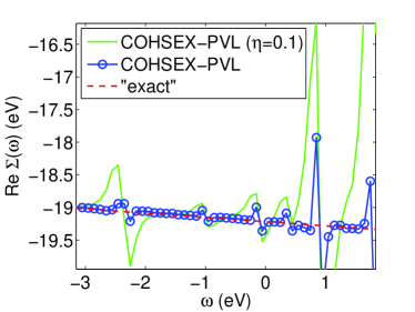
Figure 6: The real part of $\langle\phi_{4}|\Sigma(\omega)|\phi_{4}\rangle$ for a methane molecule computed by using (19) and (23) to the XCOR (left) and the COHSEX (right) expressions.

IV Conclusion

We presented a technique for performing numerical convolution of a Green’s function with a screened Coulomb potential for the GW approximation of the self energy term in a Dyson’s equation. Our numerical integration is performed directly on the real frequency axis. To overcome the difficulty associated with the singularities of the integrand, we take the zero broadening limit in Green’s function first and replace the numerator of the integrand with piecewise polynomial approximations so that the principal value integral of the approximate integrand can be obtained analytically. We presented the error bound associated with this integration scheme and showed by numerical examples that this technique produced more accurate results than standard numerical quadrature rules such as the trapezoidal rule. Consequently, to achieve the same level accuracy, fewer quadrature points are needed. This leads to a reduction in computational cost. We also showed that applying the same numerical integration to different expressions of the GW self energy approximation (e.g. the full-frequency COHSEX and XCOR) may lead to different levels of numerical accuracy. For a given frequency, one expression may be preferred over the other. Our technique has been implemented in the BerkeleyGW software package Deslippe12 , and it gives a significant improvement over the previous integration scheme. We should mention that there are other techniques for treating singularities of the integrand in the GW convolution Daling91 ; Jin99 ; Rojas95 ; Kotani02 ; Lebegue03 . We will compare the efficiency and accuracy of the technique presented in this paper with other techniques in our future work. Moreover, in this work both theoretical analysis and numerical results are for molecules. We will generalize and apply our technique to the GW approximation for solids in the future.

References

- [1] L. Hedin. New method for calculating the one-particle Green’s function with application to the electron-gas problem. Phys. Rev., 139(3A):A796, 1965.
- [2] M . S. Hybertsen and S. G. Louie. Electron correlation in semiconductors and insulators: Band gaps and quasiparticle energies. Phys. Rev. B, 34:5390, 1986.
- [3] F. Aryasetiawan and O. Gunnarsson. The GW method. Rep. Prog. Phys., 61:237, 1998.
- [4] W. G. Aulbur, L. Jönsson, and J. W. Wilkins. Quasiparticle calculations in solids. In F. Seitz, D. Turnbull, and H. Ehrenreich, editors, Solid State Physics, volume 54, page 1. Academic, New York, 2000.
- [5] G. Onida, L. Reining, and A. Rubio. Electronic excitations: density-functional versus many-body Green’s function approaches. Rev. Mod. Phys., 74:601, 2002.
- [6] L. Hedin and S. Lundqvist. Effects of electron-electron and electron-phonon interactions on the one-electron states of solids. In F. Seitz, D. Turnbull, and H. Ehrenreich, editors, Solid State Physics, volume 23, page 1. Academic Press, 1970.
- [7] R. Daling, W. van Haeringen, and B. Farid. Plasmon dispersion in silicon obtained by analytic continuation of the random-phase-approximation dielectric matrix. Phys. Rev. B, 44:2952, 1991.
- [8] Y.-G. Jin and K. J. Chang. Dynamic response function and energy-loss spectrum for Li using an N-point Padé approximant. Phys. Rev. B, 59:14841, 1999.
- [9] H. N. Rojas, R. W. Godby, and R. J. Needs. Space-time method for ab initio calculations of self-energies and dielectric response functions of solids. Phys. Rev. Lett., 74:1827, 1995.
- [10] T. Kotani and M. van Schilfgaarde. All-electron GW approximation with the mixed basis expansion based on the full-potential LMTO method. Solid State Commun., 121:461, 2002.
- [11] S. Lebégue, B. Arnaud, M. Alouani, and P. E. Bloechl. Implementation of an all-electron GW approximation based on the projector augmented wave method without plasmon pole approximation: Application to Si, SiC, AlAs, InAs, NaH, and KH. Phys. Rev. B, 67:155208, 2003.
- [12] D. Bohm and D. Pines. A collective description of electron interactions: III. Coulomb interactions in a degenerate electron gas. Phys. Rev., 92:609, 1953.
- [13] M. Gell-Mann and K.A. Brueckner. Correlation energy of an electron gas at high density. Phys. Rev., 106:364, 1957.
- [14] M. A. Woodbury. Inverting modified matrices. In Memorandum Rept., 42, page 4. Statistical Research Group, Princeton Univ., Princeton, NJ, 1950.
- [15] W. W. Hager. Updating the inverse of a matrix. SIAM Rev., 31(2):221–239, 1989.
- [16] F. Liu, L. Lin, D. Vigil-Fowler, J. Lischner, A. F. Kemper, S. Sharifzadeh, F. H. Jornada, J. Deslippe, C. Yang, J. B. Neaton, and S. G. Louie. Numerical integration for ab initio many-electron self energy calculations within the GW approximation. LBNL Report, 2014.
- [17] M. E. Casida. Time-dependent density-functional response theory for molecules. In Recent Advances in Density Functional Methods, Part I (edited by D.P. Chong), 42, page 155. World Scientific, Singapore, 1995.
- [18] M. L. Tiago and J. R. Chelikowsky. Optical excitations in organic molecules, clusters, and defects studied by first-principles Green’s function methods. Phys. Rev. B, 73:205334, 2006.
- [19] J. Lischner, J. Deslippe, M. Jain, and S. G. Louie. First-principles calculations of quasiparticle excitations of open-shell condensed matter systems. Phys. Rev. Lett., 109:036406, 2012.
- [20] C. Yang, J. C. Meza, B. Lee, and L. W. Wang. KSSOLV–a MATLAB toolbox for solving the Kohn–Sham equations. ACM Trans. Math. Software, 36:10, 2009.
- [21] M. Shishkin and G. Kresse. Implementation and performance of the frequency-dependent GW method within the PAW framework. Phys. Rev. B, 74:035101, 2006.
- [22] J. Deslippe, G. Samsonidze, D. A. Strubbe, M. Jain, M. L. Cohen, and S. G. Louie. BerkeleyGW: A massively parallel computer package for the calculation of the quasiparticle and optical properties of materials and nanostructures. Comput. Phys. Commun., 183:1269, 2012.
- [23] P. Giannozzi, S. Baroni, N. Bonini, M. Calandra, R. Car, C. Cavazzoni, D. Ceresoli, G. L. Chiarotti, M. Cococcioni, I. Dabo, A. D. Corso, S. de Gironcoli, S. Fabris, G. Fratesi, R. Gebauer, U. Gerstmann, C. Gougoussis, A. Kokalj, M. Lazzeri, L. Martin-Samos, N. Marzari, F. Mauri, R. Mazzarello, S. Paolini, A. Pasquarello, L. Paulatto, C. Sbraccia, S. Scandolo, G. Sclauzero, A. P. Seitsonen, A. Smogunov, P. Umari, and R. M. Wentzcovitch. QUANTUM ESPRESSO: a modular and open-source software project for quantum simulations of materials. J. Phys.: Condens. Matt., 39:395502, 2009.
- [24] J. P. Perdew, K. Burke, and M. Ernzerhof. Generalized gradient approximation made simple. Phys. Rev. Lett., 77:3865, 1996.
- [25] N. Troullier and J. L. Martins. Efficient pseudopotentials for plane-wave calculations. Phys. Rev. B, 43:1993, 1991.