Excitations and benchmark ensemble density functional theory for two electrons

Abstract

A new method for extracting ensemble Kohn-Sham potentials from accurate excited state densities is applied to a variety of two electron systems, exploring the behavior of exact ensemble density functional theory. The issue of separating the Hartree energy and the choice of degenerate eigenstates is explored. A new approximation, spin eigenstate Hartree-exchange (SEHX), is derived. Exact conditions that are proven include the signs of the correlation energy components, the virial theorem for both exchange and correlation, and the asymptotic behavior of the potential for small weights of the excited states. Many energy components are given as a function of the weights for two electrons in a one-dimensional flat box, in a box with a large barrier to create charge transfer excitations, in a three-dimensional harmonic well (Hooke’s atom), and for the He atom singlet-triplet ensemble, singlet-triplet-singlet ensemble, and triplet bi-ensemble.

I Introduction and illustration

Ground-state density functional theoryHK64 ; KS65 (DFT) is a popular choice for finding the ground-state energy of electronic systems,B12 and excitations can now easily be extracted using time-dependent DFTRG84 ; C96 ; MMNG12 ; U12 (TDDFT). Despite its popularity, TDDFT calculations have many well-known failings,ORR02 ; MZCB04 ; HIRC11 ; UY13 such as double excitationsEGCM11 and charge-transfer excitations.DWH03 ; T03 Alternative DFT treatments of excitationsG96 ; FHMP98 ; LN99 are always of interest.

Ensemble DFT (EDFT)T79 ; GOKb88 ; GOK88 ; OGKb88 is one such alternative approach. Unlike TDDFT, it is based on an energy variational principle. An ensemble of monotonically decreasing weights is constructed from the $M+1$ lowest levels of the system, and the expectation value of the Hamiltonian over orthogonal trial wavefunctions is minimized by the $M+1$ exact lowest eigenfunctions.GOKb88 A one-to-one correspondence can be established between ensemble densities and potentials for a given set of weights, providing a Hohenberg-Kohn theorem, and application to non-interacting electrons of the same ensemble density yields a Kohn-Sham scheme with corresponding equations.GOK88 In principle, this yields the exact ensemble energy, from which individual excitations may be extracted.

But to make a practical scheme, approximations must be used.N95 ; N98 ; SD99 ; N01 ; FF13 These have been less successful for EDFT than those of ground-stateB88 ; LYP88 ; B93 ; PBE96 ; PBE98 and TDDFT,JWPA09 ; MMNG12 and their accuracy is not yet competitive with TDDFT transition frequencies from standard approximations. Some progress has been made in identifying some major sources of error.GPG02 ; TN03 ; TNb03

To help speed up that progress, we have developed a numerical algorithm to calculate ensemble Kohn-Sham (KS) quantities (orbital energies, energy components, potentials, etc.) essentially exactly,YTPB14 from highly accurate excited-state densities. In the present paper, we provide reference KS calculations and results for two-electron systems under a variety of conditions. The potentials we find differ in significant ways from the approximations suggested so far, hopefully leading to new and better approximations.

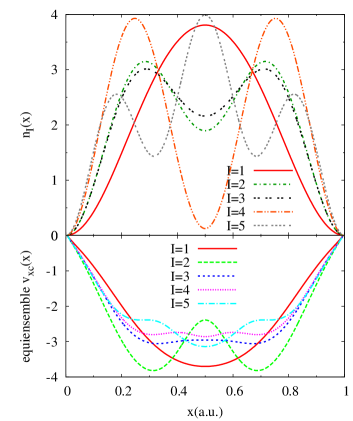
Figure 1: Exact densities and equiensemble exchange-correlation potentials of the 1D box with two electrons. The third excited state ($I=4$) is a double excitation. See Sec. VI.1.

To illustrate the essential idea, we perform calculations on simple model systems. For example, Sec. VI.1 presents two ‘electrons’ in a one-dimensional box, repelling one another via a (slightly softened) Coulomb repulsion. In Fig. 1, we show their ground- and excited-state densities, with $I$ indicating the specific ground or excited state. We also plot the ensemble exchange-correlation potentials for equally weighted mixtures of the ground and excited states, which result from our inversion scheme. In this lower plot, $I=1$ denotes the ground-state exchange-correlation potential, and $I>1$ indicates the potential corresponding to an equal mixture of the ground state and all multiplets up to and including the $I$-th state. Excitation energies for all these states are extracted using the EDFT methods described below.

The paper is laid out as follows. In the next section, we briefly review the state-of-the-art for EDFT, introducing our notation. Then we give some formal considerations about how to define the Hartree energy. The naive definition, taken directly from ground-state DFT, introduces spurious unphysical contributions (which then must be corrected-for) called ‘ghost’ corrections.GPG02 We also consider how to make choices among KS eigenstates when they are degenerate, and show that such choices matter to the accuracy of the approximations. We close that section by showing how to construct symmetry-projected ensembles.

In the following section, we prove a variety of exact conditions within EDFT. Such conditions have been vital in constructing useful approximations in ground-state DFT.LP85 ; PBE96 Following that, we describe our numerical methods in some detail.

The results section consists of calculations for quite distinct systems, but all with just two electrons. The one-dimensional flat box was used for the illustration here, which also gives rise to double excitations. A box with a high, asymmetric barrier produces charge-transfer excitations. Hooke’s atom is a three-dimensional system, containing two Coulomb-repelling electrons in a harmonic oscillator external potential.FUT94 It has proven useful in the past to test ideas and approximations in both ground-state and TDDFT calculations.HMB02 We close the section reporting several new results for the He atom, using ensembles that include low-lying triplet states. Atomic units [$e=\hbar=m_{e}=1/(4\pi\epsilon_{0})=1$] are used throughout unless otherwise specified.

II Background

II.1 Basic theory

The ensemble variational principleGOKb88 states that, for an ensemble of the lowest $M+1$ eigenstates $\Psi_{0},\ldots,\Psi_{M}$ of the Hamiltonian $\hat{H}$ and a set of orthonormal trial functions $\tilde{\Psi}_{0},\ldots,\tilde{\Psi}_{M}$,

$$\sum_{m=0}^{M}\texttt{w}_{m}\left\langle\tilde{\Psi}_{m}\left|\hat{H}\right|\tilde{\Psi}_{m}\right\rangle\geq\sum_{m=0}^{M}\texttt{w}_{m}E_{m},$$ (1)

when the set of weights $\texttt{w}_{m}$ satisfies

$$\texttt{w}_{0}\geq\texttt{w}_{1}\geq\ldots\geq\texttt{w}_{m}\geq\ldots\geq 0,$$ (2)

and $E_{m}$ is the eigenvalue of the $m$th eigenstate of $\hat{H}$. Equality holds only for $\tilde{\Psi}_{m}=\Psi_{m}$. The density matrix of such an ensemble is defined by

$$\hat{D}_{{\scriptscriptstyle\rm\mathcal{W}}}=\sum_{m=0}^{M}\texttt{w}_{m}\left|\Psi_{m}\right>\left<\Psi_{m}\right|,$$ (3)

where ${\scriptscriptstyle\rm\mathcal{W}}$ denotes the entire set of weight parameters. Properties of the ensemble are then defined as traces of the corresponding operators with the density matrix. The ensemble density $n_{\scriptscriptstyle\rm\mathcal{W}}({\bf r})$ is

$$n_{{\scriptscriptstyle\rm\mathcal{W}}}({\bf r})=\operatorname{tr}\{\hat{D}_{{\scriptscriptstyle\rm\mathcal{W}}}\hat{n}({\bf r})\}=\sum_{m=0}^{M}\texttt{w}_{m}n_{m}({\bf r}),$$ (4)

and the ensemble energy $E_{\scriptscriptstyle\rm\mathcal{W}}$ is

$$E_{{\scriptscriptstyle\rm\mathcal{W}}}=\operatorname{tr}\{\hat{D}_{{\scriptscriptstyle\rm\mathcal{W}}}\hat{H}\}=\sum_{m=0}^{M}\texttt{w}_{m}E_{m}.$$ (5)

$n_{\scriptscriptstyle\rm\mathcal{W}}({\bf r})$ is normalized to the number of electrons, implying $\sum_{m=0}^{M}\texttt{w}_{m}=1$.

A Hohenberg-Kohn (HK)HK64 type theorem for the one-to-one correspondence between $n_{\scriptscriptstyle\rm\mathcal{W}}({\bf r})$ and the potential in $\hat{H}$ has been proven,T79 ; GOK88 so all ensemble properties are functionals of $n_{\scriptscriptstyle\rm\mathcal{W}}({\bf r})$, including $\hat{D}_{{\scriptscriptstyle\rm\mathcal{W}}}$. The ensemble HK theorem allows the definition of a non-interacting KS system, which reproduces the exact $n_{\scriptscriptstyle\rm\mathcal{W}}({\bf r})$. The existence of an ensemble KS system assumes ensemble $v$-representability. EDFT itself, however, only requires ensemble non-interacting $N$-representability, since a constrained-search formalism is available.GOK88 Ensemble $N$- and $v$-representability are not yet proven, only assumed.

As in the ground-state case, only the ensemble energy functional is formally known, which is

$$E_{{\scriptscriptstyle\rm\mathcal{W}}}[n]=F_{{\scriptscriptstyle\rm\mathcal{W}}}[n]+\int\mathrm{d}^{3}r\;n({\bf r})v({\bf r}),$$ (6)

where $v({\bf r})$ is the external potential. The ensemble universal functional $F_{\scriptscriptstyle\rm\mathcal{W}}$ is defined as

$$F_{{\scriptscriptstyle\rm\mathcal{W}}}[n]=\operatorname{tr}\{\hat{D}_{{\scriptscriptstyle\rm\mathcal{W}}}[n](\hat{T}+\hat{V}_{\rm ee})\},$$ (7)

where $\hat{T}$ and $\hat{V}_{\rm ee}$ are the kinetic and electron-electron interaction potential operators, respectively. The ensemble variational principle ensures that the ensemble energy functional evaluated at the exact ensemble density associated with $v({\bf r})$ is the minimum of this functional, Eq. (5).

The ensemble KS system is defined as the non-interacting system that reproduces $n_{\scriptscriptstyle\rm\mathcal{W}}({\bf r})$ and satisfies the following non-interacting Schrödinger equation:

$$\left\{-\frac{1}{2}\nabla^{2}+v_{\text{s},{\scriptscriptstyle\rm\mathcal{W}}}[n_{{\scriptscriptstyle\rm\mathcal{W}}}]({\bf r})\right\}\phi_{j,{\scriptscriptstyle\rm\mathcal{W}}}({\bf r})=\epsilon_{j,{\scriptscriptstyle\rm\mathcal{W}}}\phi_{j,{\scriptscriptstyle\rm\mathcal{W}}}({\bf r}).$$ (8)

The ensemble KS system has the same set of $\texttt{w}_{m}$ as the interacting system. There is no formal proof for this consistency, and it has non-trivial implications even for simple systems. This will be explored more in Sec. II.2.

The KS density matrix $\hat{D}_{\text{s},{\scriptscriptstyle\rm\mathcal{W}}}$ is

$$\hat{D}_{\text{s},{\scriptscriptstyle\rm\mathcal{W}}}=\sum_{m=0}^{M}\texttt{w}_{m}\left|\Phi_{m}\right>\left<\Phi_{m}\right|,$$ (9)

where $\Phi_{m}$ are non-interacting $N$-particle wavefunctions, usually assumed to be single Slater determinants formed by KS orbitals $\phi_{j,{\scriptscriptstyle\rm\mathcal{W}}}$. We find that this choice can be problematic, and it will be discussed in Sec. III.1. The ensemble density $n_{\texttt{w}}({\bf r})$ is reproduced by the KS system, meaning

$$n_{{\scriptscriptstyle\rm\mathcal{W}}}({\bf r})=\sum_{m=0}^{M}\texttt{w}_{m}n_{m}({\bf r})=\sum_{m=0}^{M}\texttt{w}_{m}n_{\text{s},m}({\bf r}),$$ (10)

where $n_{m}({\bf r})=\left\langle\Psi_{m}\left|\hat{n}({\bf r})\right|\Psi_{m}\right\rangle$, and $n_{\text{s},m}({\bf r})=\left\langle\Phi_{m}\left|\hat{n}({\bf r})\right|\Phi_{m}\right\rangle$. The KS densities of the individual states are generally not related to those of the interacting system; only their weighted sums are equal, as in Eq. (10).

$E_{{\scriptscriptstyle\rm\mathcal{W}}}[n]$ is decomposed as in ground-state DFT,

$$\begin{split}E_{{\scriptscriptstyle\rm\mathcal{W}}}[n]&=T_{{\scriptscriptstyle\rm S},{\scriptscriptstyle\rm\mathcal{W}}}[n]+V[n]+E_{\scriptscriptstyle\rm H}[n]+E_{{\scriptscriptstyle\rm XC},{\scriptscriptstyle\rm\mathcal{W}}}[n]\\ &=\operatorname{tr}\{\hat{D}_{{\scriptscriptstyle\rm S},{\scriptscriptstyle\rm\mathcal{W}}}\hat{T}\}+\int\mathrm{d}^{3}r\;n({\bf r})v({\bf r})\\ &\quad+E_{\scriptscriptstyle\rm H}[n]+E_{{\scriptscriptstyle\rm XC},{\scriptscriptstyle\rm\mathcal{W}}}[n],\end{split}$$ (11)

where only the ensemble exchange-correlation (XC) energy $E_{{\scriptscriptstyle\rm XC},{\scriptscriptstyle\rm\mathcal{W}}}$ is unknown. The form of $v_{{\scriptscriptstyle\rm S},{\scriptscriptstyle\rm\mathcal{W}}}({\bf r})$ is then determined according to the variational principle by requiring $\delta E_{{\scriptscriptstyle\rm\mathcal{W}}}[n_{{\scriptscriptstyle\rm\mathcal{W}}}]/\delta n_{{\scriptscriptstyle\rm\mathcal{W}}}({\bf r})=0$, resulting in

$$v_{{\scriptscriptstyle\rm S},{\scriptscriptstyle\rm\mathcal{W}}}[n_{{\scriptscriptstyle\rm\mathcal{W}}}]({\bf r})=v({\bf r})+v_{\scriptscriptstyle\rm H}[n_{{\scriptscriptstyle\rm\mathcal{W}}}]({\bf r})+v_{{\scriptscriptstyle\rm XC},{\scriptscriptstyle\rm\mathcal{W}}}[n_{{\scriptscriptstyle\rm\mathcal{W}}}]({\bf r}),$$ (12)

where $v_{\scriptscriptstyle\rm H}[n]({\bf r})=\delta E_{\scriptscriptstyle\rm H}[n]/\delta n({\bf r})$, and $v_{{\scriptscriptstyle\rm XC},{\scriptscriptstyle\rm\mathcal{W}}}[n]({\bf r})=\delta E_{{\scriptscriptstyle\rm XC},{\scriptscriptstyle\rm\mathcal{W}}}[n]/\delta n({\bf r})$. $E_{\scriptscriptstyle\rm H}$ is generally defined to have the same form as the ground-state Hartree energy functional. Although this choice is reasonable, we find that it is more consistent to consider $E_{\scriptscriptstyle\rm HX}$, the combined Hartree and exchange energy. This point will be discussed in Sec. III.1.

The ensemble universal functional $F_{{\scriptscriptstyle\rm\mathcal{W}}}[n]$ depends on the set of weights $\texttt{w}_{m}$. Ref. GOK88, introduced the following set of weights, so that only one parameter w is needed:

$$\texttt{w}_{m}=\left\{\begin{array}[]{ll}\frac{1-\texttt{w}g_{I}}{M_{I}-g_{I}}&m\leq M_{I}-g_{I},\\ \texttt{w}&m>M_{I}-g_{I},\end{array}\right.$$ (13)

where $\texttt{w}\in[0,1/M_{I}]$. In this ensemble, here called GOK, $I$ denotes the set of degenerate states (or ‘multiplet’) with the highest energy in the ensemble, $g_{I}$ is the multiplicity of the $I$-th multiplet, and $M_{I}$ is the total number of states up to the $I$-th multiplet. GOK ensembles must contain full sets of degenerate states to be well-defined. The weight parameter w interpolates between two ensembles: the equiensemble up to the $I$-th multiplet ($\texttt{w}=1/M_{I}$) and the equiensemble up to the $(I-1)$-th multiplet ($\texttt{w}=0$). All previous studies of EDFT have been based on this type of ensemble.

The purpose of EDFT is to calculate excited-state properties, not ensemble properties. With the GOK ensemble, the excitation energy of multiplet $I$ from the ground state, $\omega_{I}$, is obtained using ensembles up to the $I$-th multiplet as

$$\omega_{I}=\frac{1}{g_{I}}\left.\frac{\partial E_{I,\texttt{w}}}{\partial\texttt{w}}\right|_{\texttt{w}=\texttt{w}_{I}}+\sum_{i=0}^{I-1}\frac{1}{M_{i}}\left.\frac{\partial E_{i,\texttt{w}}}{\partial\texttt{w}}\right|_{\texttt{w}=\texttt{w}_{i}},$$ (14)

which simplifies to

$$\omega_{1}=\omega_{\text{s},1,\texttt{w}}+\left.\frac{\partial E_{{\scriptscriptstyle\rm XC},\texttt{w}}[n]}{\partial\texttt{w}}\right|_{n=n_{\texttt{w}}}$$ (15)

for the first excitation energy. Eq. (14) holds for any valid ${\texttt{w}_{i}}$’s if the ensemble KS systems are exact, despite every term in Eq. (14) being w-dependent. No existing $E_{{\scriptscriptstyle\rm XC},\texttt{w}}$ approximations satisfy this condition.OGKb88 ; N98

LevyL95 pointed out that there is a special case for $\texttt{w}\to 0$ of bi-ensembles ($I=2$, with all degenerate states within a multiplet having the same density),

$$\begin{split}\Delta v_{\scriptscriptstyle\rm XC}&=\lim_{\texttt{w}\to 0}\left.\frac{\partial E_{{\scriptscriptstyle\rm XC},\texttt{w}}[n]}{\partial\texttt{w}}\right|_{n=n_{\texttt{w}}}\\ &=\left[\lim_{\texttt{w}\to 0}v_{{\scriptscriptstyle\rm XC},\texttt{w}}[n_{\texttt{w}}]({\bf r})\right]-v_{\scriptscriptstyle\rm{xc},\texttt{w}=0}[n_{\texttt{w}=0}]({\bf r})\end{split}$$ (16)

for finite $r$, where $\Delta v_{\scriptscriptstyle\rm XC}$ is the change in the KS highest-occupied-molecular-orbital (HOMO) energy between $\texttt{w}=0$ (ground state) and $\texttt{w}\to 0_{+}$.note1 $\Delta v_{\scriptscriptstyle\rm XC}$ is a property of electron-number-neutral excitations, and should not be confused with the ground-state derivative discontinuity $\Delta_{\scriptscriptstyle\rm XC}$, which is related to ionization energies and electron affinities.DG90

II.2 Degeneracies in the Kohn-Sham system

Taking the He atom as our example, the interacting system has a non-degenerate ground state, triply degenerate first excited state, and a non-degenerate second excited state. However, the KS system has a four-fold degenerate first excited state (corresponding to four Slater determinants), due to the KS singlet and triplet being degenerate (Fig. 2). Consider an ensemble of these states with arbitrary weights. Represent the ensemble energy functional Eq. (5) as the KS ensemble energy, $E_{{\scriptscriptstyle\rm S},{\scriptscriptstyle\rm\mathcal{W}}}$, plus a correction, $G_{\scriptscriptstyle\rm\mathcal{W}}$. The correction then must encode the switch from depending only on the sum of the weights of the excited states as a whole in the KS case to depending on the sum of triplet weights and the singlet weight separately.

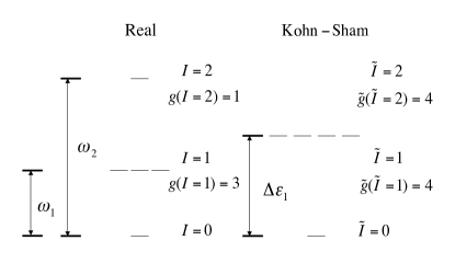
Figure 2: Diagram of the interacting and KS multiplicity structure for He. Degeneracy of the $I$-th multiplet is $g(I)$; tildes denote KS values. For instance, $\tilde{I}=2$ refers to the KS multiplet used to construct the second (singlet) multiplet of the real system ($I=2$), as is described in Sec. III.2.

For the interacting system, the ensemble energy and density take the forms

$$\begin{split}E_{\scriptscriptstyle\rm\mathcal{W}}&=\left(1-\texttt{w}_{\scriptscriptstyle\rm T}-\texttt{w}_{\scriptscriptstyle\rm S}\right)E_{0}+\texttt{w}_{\scriptscriptstyle\rm T}\omega_{1}+\texttt{w}_{\scriptscriptstyle\rm S}\omega_{2},\\ n_{\scriptscriptstyle\rm\mathcal{W}}({\bf r})&=\left(1-\texttt{w}_{\scriptscriptstyle\rm T}-\texttt{w}_{\scriptscriptstyle\rm S}\right)n_{0}({\bf r})+\texttt{w}_{\scriptscriptstyle\rm T}\Delta n_{1}({\bf r})+\texttt{w}_{\scriptscriptstyle\rm S}\Delta n_{2}({\bf r}),\end{split}$$ (17)

where $\omega_{i}=E_{i}-E_{0}$, and so on, $\texttt{w}_{\scriptscriptstyle\rm T}$ is the sum of the triplet weights, and $\texttt{w}_{\scriptscriptstyle\rm S}$ is the singlet weight. On the other hand, for the KS system we have

$$\begin{split}E_{{\scriptscriptstyle\rm S},{\scriptscriptstyle\rm\mathcal{W}}}&=\left(1-\texttt{w}_{\scriptscriptstyle\rm T}-\texttt{w}_{\scriptscriptstyle\rm S}\right)E_{\scriptscriptstyle\rm{S},0}+\left(\texttt{w}_{\scriptscriptstyle\rm T}+\texttt{w}_{\scriptscriptstyle\rm S}\right)\Delta\epsilon_{1,\texttt{w}},\\ n_{\scriptscriptstyle\rm\mathcal{W}}({\bf r})&=2\left(1-\texttt{w}_{\scriptscriptstyle\rm T}-\texttt{w}_{\scriptscriptstyle\rm S}\right)\left|\phi_{1s}\right|^{2}+\left(\texttt{w}_{\scriptscriptstyle\rm T}+\texttt{w}_{\scriptscriptstyle\rm S}\right)\left(\left|\phi_{2s}\right|^{2}-\left|\phi_{1s}\right|^{2}\right).\end{split}$$ (18)

The functional $G_{\scriptscriptstyle\rm\mathcal{W}}=E_{\scriptscriptstyle\rm\mathcal{W}}-E_{{\scriptscriptstyle\rm S},{\scriptscriptstyle\rm\mathcal{W}}}$ in this case is

$$G_{\scriptscriptstyle\rm\mathcal{W}}[n_{{\scriptscriptstyle\rm\mathcal{W}}}]=\left(1-\texttt{w}_{\scriptscriptstyle\rm T}-\texttt{w}_{\scriptscriptstyle\rm S}\right)\left(E_{0}-E_{s,0}\right)\\ +\texttt{w}_{\scriptscriptstyle\rm T}\left(\omega_{1}-\Delta\epsilon_{1}\right)+\texttt{w}_{\scriptscriptstyle\rm S}\left(\omega_{2}-\Delta\epsilon_{1}\right),$$ (19)

showing that the exact ensemble energy functional (which can also be decomposed as in Eq. (11)) has to encode the change in the multiplet structure between non-interacting and interacting systems, even for a simple system like the He atom. Such information is unknown a priori for general systems, and can be very difficult to incorporate into approximations. This problem can be alleviated if the degeneracies are the result of symmetry. This will be discussed in Sec. III.3.

II.3 Approximations

Available approximations to the ensemble $E_{\scriptscriptstyle\rm XC}$ include the quasi-local-density approximation (qLDA) functionalK86 ; OGKb88 and the ‘ghost’-corrected exact exchange (EXX) functional.N98 ; GPG02 The qLDA functional is based on the equiensemble qLDA,K86 and it interpolates between two consecutive equiensembles:OGKb88

$$E_{\scriptscriptstyle\rm{XC},I,\texttt{w}}^{\text{qLDA}}[n]({\bf r})=(1-M_{I}\texttt{w})E_{\scriptscriptstyle\rm{XC},I-1}^{\text{eqLDA}}[n]({\bf r})\\ +M_{I}\texttt{w}E_{\scriptscriptstyle\rm{XC},I}^{\text{eqLDA}}[n],$$ (20)

where $v_{\scriptscriptstyle\rm XC}^{\text{eqLDA}}({\bf r})$ is the equiensemble qLDA functional defined in terms of finite-temperature LDA in Ref. K86, .

The ensemble Hartree energy is defined analogously to the ground-state Hartree energy as shown in Eq. (11). Similarly, Nagy provides a definition of the exchange energy for bi-ensembles:N98

$$E_{{\scriptscriptstyle\rm X},\texttt{w}}^{\text{Nagy}}[n_{\uparrow},n_{\downarrow}]=-\frac{1}{2}\sum_{\sigma}\int\mathrm{d}^{3}r\mathrm{d}^{3}r^{\prime}\;\frac{\left|n_{\sigma}({\bf r},{\bf r}^{\prime})\right|^{2}}{\left|{\bf r}-{\bf r}^{\prime}\right|},$$ (21)

where $n_{\sigma}({\bf r},{\bf r}^{\prime})$ is the reduced density matrix defined analogously to its ground-state counterpart, assuming a spin-up electron is excited in the first excited state:

$$n_{\sigma,\texttt{w}}({\bf r},{\bf r}^{\prime})=\sum_{j=1}^{N_{\sigma}}n_{j,\sigma}({\bf r},{\bf r}^{\prime})+\delta_{\sigma,\uparrow}\texttt{w}\left(n_{\text{L}\uparrow}({\bf r},{\bf r}^{\prime})-n_{\text{H}\uparrow}({\bf r},{\bf r}^{\prime})\right),$$ (22)

with $n_{j,\sigma}({\bf r},{\bf r}^{\prime})=\phi_{j,\sigma}({\bf r})\phi^{*}_{j,\sigma}({\bf r}^{\prime})$, $L$$\uparrow$$=N_{\uparrow}+1$ and $H$$\uparrow$$=N_{\uparrow}$, the spin-up lowest-unoccupied-molecular-orbital (LUMO) and HOMO, respectively. Both $E_{\scriptscriptstyle\rm H}$ in Eq. (11) and (21) contain ‘ghost’ terms,GPG02 which are cross-terms between different states in the ensemble due to the summation form of $n_{\texttt{w}}({\bf r})$ in Eq. (4) and $n_{\texttt{w}}({\bf r},{\bf r}^{\prime})$ in Eq. (22). An EXX functional is obtained after such spurious terms are corrected. For two-state ensembles, the GPG XC energy functional is then

$$E_{{\scriptscriptstyle\rm X},\texttt{w}}^{\text{GPG}} [n_{\uparrow},n_{\downarrow}]=\int\frac{\mathrm{d}^{3}r\mathrm{d}^{3}r^{\prime}}{\left|{\bf r}-{\bf r}^{\prime}\right|}\left\{-\frac{1}{2}\left(n_{\sigma}({\bf r},{\bf r}^{\prime})\right)^{2}\right.$$

$$\left.+\texttt{w}\overline{\texttt{w}}\left[n_{\text{H}\uparrow}({\bf r},{\bf r}^{\prime})n_{\text{L}\uparrow}({\bf r},{\bf r}^{\prime})-n_{\text{H}\uparrow}({\bf r}^{\prime})n_{\text{H}\uparrow}({\bf r}^{\prime})\right]\right\},$$ (23)

where $\overline{\texttt{w}}=1-\texttt{w}$. These ‘ghost’ corrections are small compared to the Hartree and exchange energies. However, they are large corrections to the excitation energies, as Eq. (14) contains energy derivatives instead of energies. Table 1 shows a few examples.

With the help of the exact ensemble KS systems to be presented in this paper, we notice inconsistencies with the GPG functional. These problems and our proposed solutions will be explained in Secs. III.1 and III.2.

III Theoretical considerations

In this section, we extend EDFT to improve the consistency and generality of the theory.

III.1 Choice of Hartree energy

The energy decomposition in Eq. (11) is analogous to its ground-state counterpart. However, unlike $T_{\scriptscriptstyle\rm S}$ and $V$, the choices for $E_{\scriptscriptstyle\rm H}$ and $E_{\scriptscriptstyle\rm X}$ and $E_{\scriptscriptstyle\rm C}$ are ambiguous; only their sum is uniquely determined. As shown in Eq. (11) and (21), definitions for $E_{\scriptscriptstyle\rm H}$ and $E_{\scriptscriptstyle\rm X}$ can introduce ‘ghost’ terms. Corrections can be considered either a part of $E_{\scriptscriptstyle\rm H}$ and $E_{\scriptscriptstyle\rm X}$ or a part of $E_{\scriptscriptstyle\rm C}$. Such correction terms also take a complicated form when generalized to multi-state ensembles.

A more natural way of defining $E_{\scriptscriptstyle\rm H}$ and $E_{\scriptscriptstyle\rm XC}$ for ensembles can be achieved by considering the purpose of this otherwise arbitrary energy decomposition. In the ground-state case, the electron-electron repulsion reducesLS73 to the Hartree energy for large $Z$, which is a simple functional of the density. The remaining unknown, $E_{\scriptscriptstyle\rm XC}$ (and its components $E_{\scriptscriptstyle\rm X}$ and $E_{\scriptscriptstyle\rm C}$), is a small portion of the total energy, so errors introduced by approximations to it are small.

For ensembles, we propose a slightly different energy decomposition. Instead of defining $E_{\scriptscriptstyle\rm H}$ and $E_{\scriptscriptstyle\rm X}$ in analogy to their ground-state counterparts, we first define the combined Hartree-exchange energy $E_{\scriptscriptstyle\rm HX}$, which is the more fundamental object in EDFT. $E_{\scriptscriptstyle\rm HX}$ can be explicitly represented as the trace of the KS density matrix:

$$E_{{\scriptscriptstyle\rm HX},{\scriptscriptstyle\rm\mathcal{W}}}=\operatorname{tr}\{\hat{D}_{{\scriptscriptstyle\rm S},{\scriptscriptstyle\rm\mathcal{W}}}\hat{V}_{\rm ee}\}=\sum_{m=0}^{M}\texttt{w}_{m}\left\langle\Phi_{m}\left|\hat{V}_{\rm ee}\right|\Phi_{m}\right\rangle.$$ (24)

For the ground state, both Hartree and exchange contributions are first-order in the adiabatic coupling constant, while correlation consists of all higher-order terms. According to the definition above, we retain this property in the ensemble. Eq. (24) contains no ‘ghost’ terms by definition, eliminating the need to correct them. As a consequence, the correlation energy, $E_{\scriptscriptstyle\rm C}$, is defined and decomposed as

$$E_{{\scriptscriptstyle\rm C},{\scriptscriptstyle\rm\mathcal{W}}}=E_{{\scriptscriptstyle\rm HXC},{\scriptscriptstyle\rm\mathcal{W}}}-E_{{\scriptscriptstyle\rm HX},{\scriptscriptstyle\rm\mathcal{W}}}=T_{{\scriptscriptstyle\rm C},{\scriptscriptstyle\rm\mathcal{W}}}+U_{{\scriptscriptstyle\rm C},{\scriptscriptstyle\rm\mathcal{W}}},$$ (25)

where $E_{{\scriptscriptstyle\rm HXC},{\scriptscriptstyle\rm\mathcal{W}}}=E_{{\scriptscriptstyle\rm\mathcal{W}}}-T_{{\scriptscriptstyle\rm S},{\scriptscriptstyle\rm\mathcal{W}}}-V$, $T_{{\scriptscriptstyle\rm C},{\scriptscriptstyle\rm\mathcal{W}}}=T_{{\scriptscriptstyle\rm\mathcal{W}}}-T_{{\scriptscriptstyle\rm S},{\scriptscriptstyle\rm\mathcal{W}}}$ and $U_{{\scriptscriptstyle\rm C},{\scriptscriptstyle\rm\mathcal{W}}}=E_{{\scriptscriptstyle\rm C},{\scriptscriptstyle\rm\mathcal{W}}}-T_{{\scriptscriptstyle\rm C},{\scriptscriptstyle\rm\mathcal{W}}}$.

This form of $E_{\scriptscriptstyle\rm HX}$ reveals a deeper problem in EDFT. As demonstrated in Sec. II.2, the multiplet structure of real and KS He atoms is different. Real He has a triplet state and a singlet state as the first and second excited states, but KS He has four degenerate single Slater determinants as the first excited states. Worse, the KS single Slater determinants are not eigenstates of the total spin operator $\hat{S}^{2}$, so their ordering is completely arbitrary. The KS system is constructed to yield only the real spin densities, not other quantities. KS wavefunctions that are not eigenstates of $\hat{S}^{2}$ do not generally affect commonly calculated ground-state DFT properties,PRCS09 but things are clearly different in EDFT. Consider the bi-ensemble of the ground state and the triplet excited state of He. Then $E_{{\scriptscriptstyle\rm HX},\texttt{w}}[n_{\texttt{w}}]$ depends on which three of the four KS excited-state Slater determinants are chosen, though it must be uniquely defined. Therefore, we choose the KS wavefunctions in EDFT to be linear combinations of the degenerate KS Slater determinants, preserving spatial and spin symmetries and eliminating ambiguity in $E_{\scriptscriptstyle\rm HX}$. Such multi-determinant, spin eigenstates are also required for construction of symmetry-projected ensembles, as described in Sec. III.3.

The multi-determinant KS eigenstates and ensemble $E_{\scriptscriptstyle\rm HX}$ proposed here avoid the errors in ‘ghost’-corrected EXX,GPG02 which introduces spurious spin-polarization in closed-shell systems and inherent ambiguity in the treatment of triplet states. We observe considerable improvement in the first excitation energies of some atoms, as reported in the fourth line of Table 1.

With $E_{\scriptscriptstyle\rm HX}$ fixed, the definitions of $E_{\scriptscriptstyle\rm H}$ and $E_{\scriptscriptstyle\rm X}$ depend on one another, but $E_{\scriptscriptstyle\rm C}$ does not. Defining a Hartree functional in the same form as the ground-state

$$U[n]=\frac{1}{2}\int\mathrm{d}^{3}r\;\int\mathrm{d}^{3}r^{\prime}\;\frac{n({\bf r})n({\bf r})}{\left|{\bf r}-{\bf r}^{\prime}\right|},$$ (26)

we can examine different definitions for the GOK ensemble. We can define a ‘ghost’-free ensemble Hartree, $E_{\scriptscriptstyle\rm H}^{\text{ens}}$, as

$$E_{{\scriptscriptstyle\rm H},\texttt{w}}^{\text{ens}}=\sum_{m=0}^{M}\texttt{w}_{m}U[n_{m}],$$ (27)

i.e., the ensemble sum of the Hartree energies of the interacting densities, or the slightly different

$$E_{{\scriptscriptstyle\rm H},\texttt{w}}^{\text{KS ens}}=\sum_{m=0}^{M}\texttt{w}_{m}U[n_{\text{s},m}],$$ (28)

i.e., the ensemble sum of the Hartree energies of the KS densities. The traditional Hartree definition,

$$E^{\rm trad}_{{\scriptscriptstyle\rm H},\texttt{w}}=U[n_{\texttt{w}}],$$ (29)

introduces ‘ghost’ terms through the fictitious interaction of ground- and excited-state densities. Traditional and ensemble definitions differ in their production of ‘ghosts,’ as well as in their w-dependence. The ‘ghost’-corrected $E_{\scriptscriptstyle\rm H}$ in Ref. GPG02,

$$E_{{\scriptscriptstyle\rm H},\texttt{w}}^{\text{GPG}}=\sum_{m=0}^{M}\texttt{w}_{m}^{2}U[n_{\text{s},m}]$$ (30)

has a different form from Eq. (28), which is also ‘ghost’-free. Each of these definitions of $E_{\scriptscriptstyle\rm H}$ reduces to the ground-state $E_{\scriptscriptstyle\rm H}$ when $\texttt{w}_{0}=1$ and satisfies simple inequalities such as $E_{\scriptscriptstyle\rm H}>0$ and $E_{\scriptscriptstyle\rm X}<0$. However, this ambiguity in the definition of $E_{\scriptscriptstyle\rm H}$ requires that an approximated ensemble $E_{\scriptscriptstyle\rm XC}$ be explicit about its compatible $E_{\scriptscriptstyle\rm H}$ definition.

The different flavors of $E_{{\scriptscriptstyle\rm H},\texttt{w}}$ are compared for the He singlet ensembleYTPB14 in Fig. 3. Even though $E_{{\scriptscriptstyle\rm H},\texttt{w}}^{\text{ens}}$ and $E_{{\scriptscriptstyle\rm H},\texttt{w}}^{\text{KS ens}}$ do not contain ‘ghost’ terms by definition, their magnitude is slightly bigger than that of $E_{\text{H}}^{\text{trad}}$, which is not ‘ghost’-free. This apparent contradiction stems from $E_{{\scriptscriptstyle\rm H},\texttt{w}}^{\text{ens}}$ and $E_{{\scriptscriptstyle\rm H},\texttt{w}}^{\text{KS ens}}$ depending linearly on w, while $E_{{\scriptscriptstyle\rm H},\texttt{w}}^{\text{trad}}$ depends on w quadratically. The quadratic dependence on w is made explicit with the ‘ghost’-corrected $E_{{\scriptscriptstyle\rm H},\texttt{w}}^{\text{GPG}}$ of Ref. GPG02, . Comparing with the ‘ghost’-free $E_{{\scriptscriptstyle\rm H},\texttt{w}}^{\text{ens}}$ and $E_{{\scriptscriptstyle\rm H},\texttt{w}}^{\text{KS ens}}$, it is clear that $E_{\scriptscriptstyle\rm H}^{\text{GPG}}$ overcorrects in a sense, and is compensated by an over-correction of the opposite direction in $E_{\scriptscriptstyle\rm X}^{\text{GPG}}$ (see Supplemental Material).

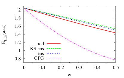
Figure 3: Behaviors of the different ensemble Hartree energy definitions for the singlet ensemble of He.

The traditional definition of Eq. (29) has the advantage that $v_{\scriptscriptstyle\rm H}({\bf r})$ is a simple functional derivative with respect to the ensemble density. Any other definition requires solving an optimized effective potential (OEP)SH53 ; TS76 -type equation to obtain $v_{\scriptscriptstyle\rm H}$. On the other hand, an approximated $E_{\scriptscriptstyle\rm XC}$ compatible with $E_{\scriptscriptstyle\rm H}^{\text{trad}}$ requires users to approximate the corresponding ‘ghost’ correction as part of $E_{\scriptscriptstyle\rm XC}$. Since the ghost correction is usually non-negligible, this is a major source of error for the qLDA functional.

III.2 Symmetry-eigenstate Hartree-exchange (SEHX)

As mentioned previously, the ‘ghost’-corrected EXX of Ref. GPG02, introduces spurious spin-polarization even for closed-shell systems. The root of this problem is the use of single-Slater-determinant wavefunctions, which are not symmetry eigenstates. We have now identified $E_{\scriptscriptstyle\rm HX}$ as being more consistent with the EDFT formalism than $E_{\scriptscriptstyle\rm H}$ and $E_{\scriptscriptstyle\rm X}$. Having also justified multi-determinant ensemble KS wavefunctions, we now derive a spin-consistent EXX potential, the symmetry-eigenstate Hartree-exchange (SEHX). Define the two-electron repulsion integral

$$\left(\mu\nu\mid\kappa\lambda\right)=\int\frac{\mathrm{d}^{3}r\mathrm{d}^{3}r^{\prime}}{\left|{\bf r}-{\bf r}^{\prime}\right|}\phi^{*}_{\mu}({\bf r})\phi^{*}_{\nu}({\bf r}^{\prime})\phi_{\kappa}({\bf r})\phi_{\lambda}({\bf r}^{\prime})$$ (31)

and

$$L_{\mu\nu\kappa\lambda}=\left(\mu\nu\mid\kappa\lambda\right)\delta_{\sigma_{\mu},\sigma_{\kappa}}\delta_{\sigma_{\nu},\sigma_{\lambda}}.$$ (32)

$\phi_{\mu}({\bf r})$ denotes the $\mu$-th KS orbital and $\sigma_{\mu}$ its spin state. If the occupation of the $p$-th Slater determinant of the $\mu$-th KS orbital of the $\tilde{i}$-th multiplet of the exact system is $f_{p\mu}^{(\tilde{i})}$, define

$$\alpha_{\mu,\nu}^{(i,k)}=\sum_{p=1}^{\tilde{g}(\tilde{i})}C_{p}^{(i,k)}f_{p,\mu}^{(\tilde{i})}f_{p,\nu}^{(\tilde{i})},$$ (33)

where $\tilde{g}(\tilde{i})$ is the KS multiplicity of the $i$-th multiplet, and $C$’s are the coefficients of the multi-determinant wavefunctions defined by

$$\Psi_{\text{s}}^{(i,k)}({\bf r}_{1},\ldots,{\bf r}_{N})=\sum_{p=1}^{\tilde{g}(\tilde{i})}C^{(i,k)}_{p}\tilde{\Psi}_{\text{s},p}^{\tilde{i}}({\bf r}_{1},\ldots,{\bf r}_{N}).$$ (34)

$\tilde{\Psi}_{\text{s}}$ is a KS single Slater determinant. Note the numbering of the KS multiplets, $\tilde{i}$, depends on $i$, the numbering of the exact multiplet structure. The $C$ coefficients are chosen according to the spatial and spin symmetries of the exact state. Now, with $p$ and $q$ KS single Slater determinants of the KS multiplet, define

$$h^{(i,k)}_{\mu\nu\kappa\lambda} =\left(\alpha^{(i,k)}_{\mu,\nu}\alpha^{(i,k)}_{\kappa,\lambda}-\sum_{q=1}^{\tilde{g}(\tilde{i})}\left(C_{q}^{(i,k)}\right)^{2}f_{q,\mu}^{(\tilde{i})}f_{q,\nu}^{(\tilde{i})}f_{q,\kappa}^{(\tilde{i})}f_{q,\lambda}^{(\tilde{i})}\right)$$

$$\times\prod_{\eta\neq\mu,\nu,\kappa,\lambda}^{\tilde{g}(\tilde{i})}\delta_{f_{p,\eta}^{\tilde{i}},f_{q,\eta}^{\tilde{i}}},$$ (35)

in order to write

$$H^{(i,k)}=\sum_{\begin{subarray}{c}\mu,\nu>\mu\\ \kappa,\lambda>\kappa\end{subarray}}\left(L_{\mu\nu\kappa\lambda}-L_{\mu\nu\lambda\kappa}\right)h^{(i,k)}_{\mu\nu\kappa\lambda}.$$ (36)

Then, if

$$G^{(i,k)}=\sum_{\mu,\nu>\mu}\left(L_{\mu\mu\nu\nu}-\Re{L_{\mu\nu\mu\nu}}\right)\sum_{p=1}^{\tilde{g}(\tilde{i})}\left|C_{p}^{(i,k)}\right|^{2}f^{\tilde{i}}_{p,\mu}f^{\tilde{i}}_{p,\nu},$$ (37)

the Hartree-exchange energy for up to the $I$-th multiplet is

$$E_{{\scriptscriptstyle\rm HX},{\scriptscriptstyle\rm\mathcal{W}}}^{\text{SEHX}}=\sum_{i=1}^{I}\sum_{k=1}^{g(i)}\texttt{w}^{(i,k)}\left\{G^{(i,k)}+H^{(i,k)}\right\},$$ (38)

where $g(i)$ is the exact multiplicity of the $i$-th multiplet. The $v_{{\scriptscriptstyle\rm HX},{\scriptscriptstyle\rm\mathcal{W}}}$ potential is then

$$\begin{split}v_{\scriptscriptstyle\rm{HX},{\scriptscriptstyle\rm\mathcal{W}},\sigma}^{\text{SEHX}}({\bf r})&=\frac{\delta E_{{\scriptscriptstyle\rm HX},{\scriptscriptstyle\rm\mathcal{W}}}}{\delta n_{{\scriptscriptstyle\rm\mathcal{W}},\sigma}({\bf r})}\\ &=\int\mathrm{d}^{3}r^{\prime}\;\sum_{j}\frac{\delta E_{{\scriptscriptstyle\rm HX},{\scriptscriptstyle\rm\mathcal{W}}}}{\delta\phi_{j,\sigma}({\bf r}^{\prime})}\frac{\delta\phi_{j,\sigma}({\bf r}^{\prime})}{\delta n_{{\scriptscriptstyle\rm\mathcal{W}},\sigma}({\bf r})}+\text{c.c.},\end{split}$$ (39)

which yields an OEP-type equation for $v_{{\scriptscriptstyle\rm HX},{\scriptscriptstyle\rm\mathcal{W}}}({\bf r})$.

The $v_{{\scriptscriptstyle\rm HX},{\scriptscriptstyle\rm\mathcal{W}}}({\bf r})$ of Eq. (39) produces neither ‘ghost’ terms nor spurious spin-polarizations. For closed-shell systems, Eq. (39) yields $v_{\scriptscriptstyle\rm{HX},{\scriptscriptstyle\rm\mathcal{W}},\uparrow}({\bf r})=v_{\scriptscriptstyle\rm{HX},{\scriptscriptstyle\rm\mathcal{W}},\downarrow}({\bf r})$, unlike Ref. GPG02, . An explicit $v_{{\scriptscriptstyle\rm HX},{\scriptscriptstyle\rm\mathcal{W}}}({\bf r})$ can be obtained by applying the usual Krieger-Li-Iafrate(KLI)KLI90 approximation. Here we provide the example of the singlet bi-ensemble studied in our previous paper.YTPB14 $E_{\scriptscriptstyle\rm HX}$ for a closed-shell, singlet ensemble is

$$E_{{\scriptscriptstyle\rm HX},\texttt{w}}^{\text{SEHX}}=\int\frac{\mathrm{d}^{3}r\mathrm{d}^{3}r^{\prime}}{\left|{\bf r}-{\bf r}^{\prime}\right|}\left\{n^{\text{orb}}_{1}({\bf r})n^{\text{orb}}_{1}({\bf r}^{\prime})\right.\\ +\texttt{w}\left[n^{\text{orb}}_{1}({\bf r})\left(n^{\text{orb}}_{2}({\bf r}^{\prime})-n^{\text{orb}}_{1}({\bf r}^{\prime})\right)\right.\\ \left.\left.+\phi_{1}^{*}({\bf r})\phi_{2}^{*}({\bf r}^{\prime})\phi_{1}({\bf r}^{\prime})\phi_{2}({\bf r})\right]\right\},$$ (40)

where $n^{\text{orb}}_{j}({\bf r})=\left|\phi_{j}({\bf r})\right|^{2}$ is the KS orbital density. Spin is not explicitly written out because the system is closed-shell. After applying the KLI approximation, we obtain

$$v_{{\scriptscriptstyle\rm HX},\texttt{w}}({\bf r})=\frac{1}{2n_{\texttt{w}}({\bf r})}\left\{(2-\texttt{w})n^{\text{orb}}_{1}({\bf r})\left[v_{1}({\bf r})+\bar{v}_{\scriptscriptstyle\rm{HX}1}-\bar{v}_{1}\right]\right.\\ \left.+\texttt{w}~{}n^{\text{orb}}_{2}({\bf r})\left[v_{2}({\bf r})+\bar{v}_{\scriptscriptstyle\rm{HX}2}-\bar{v}_{2}\right]\right\},$$ (41)

with

$$v_{1}({\bf r})=\frac{1}{(2-\texttt{w})}\int\frac{\mathrm{d}^{3}r^{\prime}}{\left|{\bf r}-{\bf r}^{\prime}\right|}\left[2(1-\texttt{w})n^{\text{orb}}_{1}({\bf r}^{\prime})\right.\\ \left.+\texttt{w}\left(n^{\text{orb}}_{2}({\bf r}^{\prime})+\phi_{1}^{*}({\bf r}^{\prime})\phi_{2}^{*}({\bf r})\phi_{2}({\bf r}^{\prime})/\phi_{1}^{*}({\bf r})\right)\right],$$ (42)

$$v_{2}({\bf r})=\int\frac{\mathrm{d}^{3}r^{\prime}}{\left|{\bf r}-{\bf r}^{\prime}\right|}\left[n^{\text{orb}}_{1}({\bf r}^{\prime})+\frac{\phi_{1}^{*}({\bf r})\phi_{2}^{*}({\bf r}^{\prime})\phi_{1}({\bf r}^{\prime})}{\phi_{2}^{*}({\bf r})}\right],$$ (43)

and

$$\bar{v}_{j}=\int\mathrm{d}^{3}r\;v_{j}({\bf r})n^{\text{orb}}_{j}({\bf r}).$$ (44)

Eq. (41) is an integral equation for $v_{\scriptscriptstyle\rm HX}({\bf r})$ that can be easily solved.

To fully understand the performance of $v_{\scriptscriptstyle\rm HX}({\bf r})$, self-consistent EDFT calculations would be needed at different values of w, which is beyond the scope of this paper. We demonstrate the performance at $\texttt{w}=0$ later in Sec. IV.4.

III.3 Symmetry-projected Hamiltonian

The ensemble variational principle holds for any Hamiltonian. If the Hamiltonian $\hat{H}$ commutes with another operator $\hat{O}$, one can apply to $\hat{H}$ a projection operator formed by the eigenvectors of $\hat{O}$. One obtains a new Hamiltonian, and the ensemble variational principle holds for this subspace of $\hat{H}$, allowing an EDFT to be formulated.

An example would be the total spin operator $\hat{S}^{2}$, where

$$S^{2}=\sum_{S=0}^{\infty}(2S+1)\left|S\right>\left<S\right|$$ (45)

and $\left|S\right>$ are its eigenvectors. Define a new Hamiltonian $\hat{H}_{1}$ as

$$\hat{H}_{1}=\left|S\right>\left<S\right|\hat{H}.$$ (46)

$\hat{H}_{1}$ has the same set of eigenvectors as $\hat{H}$, but the eigenvalues are 0 for the eigenvectors not having spin $S$. Since one can change the additive constant in $\hat{H}$ arbitrarily, it is always possible to make the eigenvalues of any set of spin-$S$ eigenvectors negative and thus ensure that they are the lowest energy states of $\hat{H}_{1}$. The ensemble variational principle holds for ensembles of spin-$S$ states. We have employed this symmetry argument in our previous paperYTPB14 for a purely singlet two-state ensemble of the He atom.

A similar statement is available in ground-state DFT, allowing direct calculation of the lowest state of a certain symmetry.Gunnarsson1976 ; Goerling1993 The differences between the subspace and full treatments are encoded in the differences in their corresponding $E_{\scriptscriptstyle\rm XC}$. Thus the lowest two states within each spatial and spin symmetry category can be treated in EDFT in a two-state-ensemble fashion, which is vastly simpler than the multi-state formalism.

Since the multiplet structures of the interacting system and the KS system must be compatible, a symmetry-projected ensemble also requires a symmetry-projected KS system, which is impossible if KS wavefunctions are single Slater determinants, as discussed in Sec. III.1.

IV Exact conditions

Here we prove some basic relations for the signs of various components of the KS scheme and a virial for the potentials. We describe a feature of the ensemble derivative discontinuity and extraction of excited properties from the ground state.

IV.1 Inequalities

Simple exact inequalities of the energy components (such as $E_{\scriptscriptstyle\rm C}<0$) have been proven in ground-state DFT.DG90 If these are true in EDFT, experiences designing approximated $E_{\scriptscriptstyle\rm XC}$ in ground-state DFT may be transferrable to EDFT. Here we show that inequalities related to the correlation energy are still valid in EDFT.

Due to the variational principle,GOKb88 the wavefunctions that minimize the ensemble energy Eq. (5) are the interacting wavefunctions $\Psi_{m}$. Thus

$$E_{{\scriptscriptstyle\rm C},{\scriptscriptstyle\rm\mathcal{W}}}=\operatorname{tr}\{\hat{D}_{{\scriptscriptstyle\rm\mathcal{W}}}\hat{H}\}-\operatorname{tr}\{\hat{D}_{{\scriptscriptstyle\rm S},{\scriptscriptstyle\rm\mathcal{W}}}\hat{H}\}\leq 0.$$ (47)

The existence of a non-interacting KS systemGOK88 means $T_{{\scriptscriptstyle\rm S},{\scriptscriptstyle\rm\mathcal{W}}}$ is the smallest possible kinetic energy for a given density $n_{\scriptscriptstyle\rm\mathcal{W}}({\bf r})$, resulting in

$$T_{{\scriptscriptstyle\rm C},{\scriptscriptstyle\rm\mathcal{W}}}=T_{{\scriptscriptstyle\rm\mathcal{W}}}-T_{{\scriptscriptstyle\rm S},{\scriptscriptstyle\rm\mathcal{W}}}\geq 0.$$ (48)

From Eq. (47) and (48) we immediately obtain

$$U_{{\scriptscriptstyle\rm C},{\scriptscriptstyle\rm\mathcal{W}}}=E_{{\scriptscriptstyle\rm C},{\scriptscriptstyle\rm\mathcal{W}}}-T_{{\scriptscriptstyle\rm C},{\scriptscriptstyle\rm\mathcal{W}}}\leq 0,$$ (49)

and

$$\left|U_{{\scriptscriptstyle\rm C},{\scriptscriptstyle\rm\mathcal{W}}}\right|\geq\left|T_{{\scriptscriptstyle\rm C},{\scriptscriptstyle\rm\mathcal{W}}}\right|.$$ (50)

These inequalities are later verified with exact ensemble KS calculations.

IV.2 Virial Theorem

Since EDFT is a variational method, one expects that the virial theorem holds. A brief argument was given in Ref. YTPB14, , but we provide a straightforward proof here. We apply the usual coordinate scaling on the wavefunctions:PY89

$$\Psi_{m,\gamma}({\bf r}_{1},\ldots,{\bf r}_{N})=\gamma^{3N/2}\Psi_{m}(\gamma{\bf r}_{1},\ldots,\gamma{\bf r}_{N}).$$ (51)

According to the variational principle, the exact interacting wavefunctions $\Psi_{m}$ minimize the ensemble energy $E_{{\scriptscriptstyle\rm\mathcal{W}}}$ for a given set ${\scriptscriptstyle\rm\mathcal{W}}$. First-order variations of the ensemble energy therefore vanish. Thus

$$\left.\frac{d}{d\gamma}\operatorname{tr}\{\hat{D}_{{\scriptscriptstyle\rm\mathcal{W}},\gamma}\hat{H}\}\right|_{\gamma=1}=0,$$ (52)

where $\hat{D}_{{\scriptscriptstyle\rm\mathcal{W}},\gamma}=\sum_{m=0}^{M}\texttt{w}_{m}\left|\Psi_{m,\gamma}\right>\left<\Psi_{m,\gamma}\right|$. Since $\hat{H}=\hat{T}+\hat{V}_{\scriptscriptstyle\rm tot}=\hat{T}+\hat{V}+\hat{V}_{\rm ee}$, we have

$$\left.\frac{d}{d\gamma}\operatorname{tr}\{\hat{D}_{{\scriptscriptstyle\rm\mathcal{W}}}\}(\gamma^{2}\hat{T}+\gamma\hat{V}_{\scriptscriptstyle\rm tot})\}\right|_{\gamma=1}=0,$$ (53)

yielding

$$2T_{{\scriptscriptstyle\rm\mathcal{W}}}[n_{{\scriptscriptstyle\rm\mathcal{W}}}]+V_{\text{ee},{\scriptscriptstyle\rm\mathcal{W}}}[n_{{\scriptscriptstyle\rm\mathcal{W}}}]=\int\mathrm{d}^{3}r\;n_{{\scriptscriptstyle\rm\mathcal{W}}}({\bf r}){\bf r}\cdot\nabla v({\bf r}).$$ (54)

We can write the energy of an ensemble for a given set of weights ${\scriptscriptstyle\rm\mathcal{W}}$ and a given coupling constant $\lambda$ as

$$E_{{\scriptscriptstyle\rm\mathcal{W}}}^{\lambda}[n]=F_{{\scriptscriptstyle\rm\mathcal{W}}}^{\lambda}[n]+\int\mathrm{d}^{3}r\;n({\bf r})v_{{\scriptscriptstyle\rm\mathcal{W}}}^{\lambda}({\bf r}),$$ (55)

where $v_{{\scriptscriptstyle\rm\mathcal{W}}}^{\lambda}({\bf r})$ is the ${\scriptscriptstyle\rm\mathcal{W}}$-dependent, one-body potential maintaining a constant density for all degrees of interaction.LP85 $v_{{\scriptscriptstyle\rm\mathcal{W}}}^{\lambda=0}({\bf r})=v_{{\scriptscriptstyle\rm S},{\scriptscriptstyle\rm\mathcal{W}}}({\bf r})$, and $v_{{\scriptscriptstyle\rm\mathcal{W}}}^{\lambda=1}({\bf r})=v({\bf r})$. The functional derivative of Eq. (55) with respect to $n({\bf r})$ is

$$\frac{\delta E_{{\scriptscriptstyle\rm\mathcal{W}}}^{\lambda}}{\delta n({\bf r})}=\frac{\delta F_{{\scriptscriptstyle\rm\mathcal{W}}}^{\lambda}}{\delta n({\bf r})}+v_{{\scriptscriptstyle\rm\mathcal{W}}}^{\lambda}({\bf r}).$$ (56)

Thus

$$-\int\mathrm{d}^{3}r\;n({\bf r}){\bf r}\cdot\nabla\left[\frac{\delta F_{{\scriptscriptstyle\rm\mathcal{W}}}^{\lambda}}{\delta n({\bf r})}\right]=\int\mathrm{d}^{3}r\;n({\bf r}){\bf r}\cdot\nabla v_{{\scriptscriptstyle\rm\mathcal{W}}}^{\lambda}({\bf r}).$$ (57)

Applying the ensemble virial theorem of Eq. (54) to Eq. (57) yields

$$-\int\mathrm{d}^{3}r\;n({\bf r}){\bf r}\cdot\nabla\left[\frac{\delta F_{\scriptscriptstyle\rm\mathcal{W}}^{\lambda}}{\delta n({\bf r})}\right]=F_{\scriptscriptstyle\rm\mathcal{W}}^{\lambda}[n]+T_{\scriptscriptstyle\rm\mathcal{W}}^{\lambda}[n].$$ (58)

Considering the KS quantities, we can insert the energy in terms of Hartree-exchange-correlation and the $\lambda$-dependent one-body potential into the general virial:

$$2T_{{\scriptscriptstyle\rm\mathcal{W}}}^{\lambda}[n]=-\lambda E_{{\scriptscriptstyle\rm HXC},{\scriptscriptstyle\rm\mathcal{W}}}^{\lambda}[n]+\lambda T_{{\scriptscriptstyle\rm C},{\scriptscriptstyle\rm\mathcal{W}}}^{\lambda}[n]+\int d^{3}r\;n({\bf r}){\bf r}\cdot\nabla v_{{\scriptscriptstyle\rm\mathcal{W}}}^{\lambda}({\bf r}).$$ (59)

After this, set $\lambda=1$ for the physical system,

$$2T_{{\scriptscriptstyle\rm\mathcal{W}}}[n]=-E_{{\scriptscriptstyle\rm HXC},{\scriptscriptstyle\rm\mathcal{W}}}[n]+T_{{\scriptscriptstyle\rm C},{\scriptscriptstyle\rm\mathcal{W}}}[n]+\int d^{3}r\;n({\bf r}){\bf r}\cdot\nabla v_{{\scriptscriptstyle\rm\mathcal{W}}}({\bf r}),$$ (60)

and $\lambda=0$ for KS,

$$2T_{{\scriptscriptstyle\rm S},{\scriptscriptstyle\rm\mathcal{W}}}[n]=\int d^{3}r\;n({\bf r}){\bf r}\cdot\nabla v_{{\scriptscriptstyle\rm S},{\scriptscriptstyle\rm\mathcal{W}}}({\bf r}),$$ (61)

and subtract. This yields

$$T_{{\scriptscriptstyle\rm C},{\scriptscriptstyle\rm\mathcal{W}}}[n]=-E_{{\scriptscriptstyle\rm HXC},{\scriptscriptstyle\rm\mathcal{W}}}[n]-\int d^{3}r\;n({\bf r}){\bf r}\cdot\nabla v_{{\scriptscriptstyle\rm HXC},{\scriptscriptstyle\rm\mathcal{W}}}({\bf r})$$ (62)

and

$$E_{{\scriptscriptstyle\rm HX},{\scriptscriptstyle\rm\mathcal{W}}}[n]=-\int d^{3}r\;n({\bf r}){\bf r}\cdot\nabla v_{{\scriptscriptstyle\rm HX},{\scriptscriptstyle\rm\mathcal{W}}}({\bf r}).$$ (63)

Finally, the virial theorem for the correlation energy takes a similar form as in ground-state DFT:

$$T_{{\scriptscriptstyle\rm C},{\scriptscriptstyle\rm\mathcal{W}}}[n]=-E_{{\scriptscriptstyle\rm C},{\scriptscriptstyle\rm\mathcal{W}}}[n]-\int d^{3}r\;n({\bf r}){\bf r}\cdot\nabla v_{{\scriptscriptstyle\rm C},{\scriptscriptstyle\rm\mathcal{W}}}({\bf r}).$$ (64)

Energy densities have been important interpretation tools in ground-state DFT, and here we provide similar tools for EDFT. The integrand of Eq. (62) can be interpreted as an energy density, since integrating over all space gives

$$\begin{split}E_{{\scriptscriptstyle\rm HXC},{\scriptscriptstyle\rm\mathcal{W}}}+T_{{\scriptscriptstyle\rm C},{\scriptscriptstyle\rm\mathcal{W}}}&=\int d^{3}r\left(e_{{\scriptscriptstyle\rm HXC},{\scriptscriptstyle\rm\mathcal{W}}}+t_{{\scriptscriptstyle\rm C},{\scriptscriptstyle\rm\mathcal{W}}}\right)\\ &=-\int d^{3}r~{}n({\bf r}){\bf r}\cdot\nabla v_{{\scriptscriptstyle\rm HXC},{\scriptscriptstyle\rm\mathcal{W}}}({\bf r}),\end{split}$$ (65)

which can easily be converted to an “unambiguous” energy density.BCL98

IV.3 Asymptotic behavior

Ref. L95, derived the ensemble derivative discontinuity of Eq. (16) for bi-ensembles, in the limit of $\texttt{w}\to 0$. For finite w of an atomic system, as shown in our previous paper,YTPB14 $\Delta v_{\scriptscriptstyle\rm XC}$ is close to a finite constant for small $r$, and jumps to 0 at some position denoted by $r_{\scriptscriptstyle\rm C}$. We provide the derivation of the location of $r_{\scriptscriptstyle\rm C}$ as a function of w here.

For atoms, the HOMO wavefunction and LUMO wavefunctions have the following behavior:

$$\begin{split}\phi_{\text{HOMO}}({\bf r})&\sim Ar^{\beta}e^{-\alpha r}\\ \phi_{\text{LUMO}}({\bf r})&\sim A^{\prime}r^{\beta^{\prime}}e^{-\alpha^{\prime}r},\end{split}$$ (66)

with $\alpha\geq\alpha^{\prime}$. For the bi-ensemble of the ground state and the first excited state, the ensemble density is

$$n_{\texttt{w}}({\bf r})\sim 2\sum_{n=1}^{\text{HOMO}}\left|\phi_{n}({\bf r})\right|^{2}\\ +\texttt{w}\left(A^{\prime 2}r^{2\beta^{\prime}}e^{-2\alpha^{\prime}r}-A^{2}r^{2\beta}e^{-2\alpha r}\right),\quad r\rightarrow\infty,$$ (67)

assuming that the HOMO is doubly-occupied. The behavior of the density at large $r$ is dominated by the density of the doubly-occupied HOMO and the second term. In order to see where the density decay switches from that of the HOMO to the LUMO, we find the $r$-value at which the two differently decaying contributions are equal:

$$\left(2-\texttt{w}\right)A^{2}r^{2\beta}e^{-2\alpha r}=\texttt{w}A^{\prime 2}r^{2\beta^{\prime}}e^{-2\alpha r}.$$ (68)

As $\texttt{w}\to 0$, $r_{\scriptscriptstyle\rm C}$ is then

$$r_{\scriptscriptstyle\rm C}\to-\frac{\ln{\texttt{w}}}{2\Delta\alpha},$$ (69)

with $\Delta\alpha=\alpha-\alpha^{\prime}$.

The ionization energies are available for the He ground state and singlet excited state. Since

$$n({\bf r})\sim e^{-2\alpha r}\approx e^{-2\sqrt{2I}r},$$ (70)

we obtain

$$r_{\scriptscriptstyle\rm C}\to-0.621\ln\texttt{w},\quad\texttt{w}\to 0.$$ (71)

for the He singlet bi-ensemble with w close to 0.

IV.4 Connection to ground-state DFT

With weights as in Eq. (13), calculation of the excitation energies is done recursively: for the $M$th excited state, one needs to perform an EDFT calculation with the $M$th state highest in the ensemble, and another EDFT calculation with the $(M-1)$th as the highest state, and so on. Thus for the $M$th state, one needs to perform $M$ separate EDFT calculations for its excitation energy.

For bi-ensembles, however, the calculation of the excitation energy can be greatly simplified. Eq. (14) holds for $\texttt{w}=0$, so one can work with ground-state data only and obtain the first-excited state energy, without the need for an explicit EDFT calculation of the two-state ensemble.

We calculate the first excitation energies of various atoms and ions with Eq. (14) at $\texttt{w}=0$ with both qLDAOGKb88 ; K86 (based on LDA ground states), EXX,N98 GPG,GPG02 and SEHX, with the last three based on OEP-EXX (KLI) ground states.KLI90 In order to ensure the correct symmetry in the end result, SEHX must be performed on spin-restricted ground states. However, for closed-shell systems, these results coincide with those of spin-unrestricted calculations. We use these readily available results when possible in this paper. The w-derivatives of the $E_{\scriptscriptstyle\rm XC}$’s for qLDA and EXX required in Eq. (14) are (considering Eq. (76))

$$\lim_{\texttt{w}\to 0}\left.\frac{\partial E_{{\scriptscriptstyle\rm XC},\texttt{w}}^{\text{qLDA}}[n]}{\partial\texttt{w}}\right|_{n=n_{\texttt{w}}}=M_{I}\left(E_{\scriptscriptstyle\rm XC}^{\text{eqLDA}}[I=2,n]-E_{\scriptscriptstyle\rm XC}^{\text{LDA}}[n]\right),$$ (72)

where $E_{\scriptscriptstyle\rm XC}^{\text{LDA}}$ is the ground-state LDA functional, and

$$\lim_{\texttt{w}\to 0}\left.\frac{\partial E_{{\scriptscriptstyle\rm X},\texttt{w}}^{\text{GPG}}[n]}{\partial\texttt{w}}\right|_{n=n_{\texttt{w}}}=\int\!\!\int\frac{\mathrm{d}^{3}r\mathrm{d}^{3}r^{\prime}}{\left|{\bf r}-{\bf r}^{\prime}\right|}$$ (73)

$$\times\Bigg{\{}\left[\sum_{j=1}^{N^{\uparrow}}n_{j}({\bf r},{\bf r}^{\prime})\right]\left[n_{\text{H}}({\bf r},{\bf r}^{\prime})-n_{\text{L}}({\bf r},{\bf r}^{\prime})\right]$$

$$-n_{\text{H}}({\bf r})n_{\text{L}}({\bf r}^{\prime})+n_{\text{H}}({\bf r},{\bf r}^{\prime})n_{\text{L}}({\bf r},{\bf r}^{\prime})\Bigg{\}}$$

$$+\int\mathrm{d}^{3}r\;v_{\scriptscriptstyle\rm XC}({\bf r})[n_{\text{H}}({\bf r})-n_{\text{L}}({\bf r})],$$

where $j$ sums over the spin-up densities. Only ground state properties are needed to evaluate Eq. (73). The results are listed in Table 1. SEHX improves calculated excitation energies for systems where GPG has large errors, such as Be and Mg atoms.

	He	Li	Li+	Be	Be+	Mg	Ca	Ne	Ar
Exp.	20.62	1.85	60.76	5.28	3.96	4.34	2.94	16.7	11.6
qLDA	-	1.93	53.85	3.71	4.30	3.58	1.79	14.2	10.7
EXX	27.30	6.34	72.26	10.22	12.38	8.25	9.89	26.0	18.2
GPG	20.67	1.84	60.40	3.53	4.00	3.25	3.25	18.2	12.1
SEHX	20.67	2.08∗	60.40	5.25	4.06∗	4.39	3.55	18.4	12.2

Table 1: First non-triplet excitation energies (in eV) of various atoms and ions calculated with qLDA, EXX, GPG, and SEHX functionals. qLDA calculations were performed upon LDA (PW92)PW92 ground states; EXXN98 ground states were used for the rest. Asterisks indicate use of spin-restricted ground states. qLDA relies on ground-state LDA orbital energy differences; it cannot be used with the single bound orbital of LDA He.

V Numerical procedure

We invert the ensemble KS equation with exact densities to obtain the exact KS potential. We describe the numerical inversion procedure in Ref. YTPB14, . For ease in obtaining the Hartree potential, $E_{\scriptscriptstyle\rm H}$ is always chosen to be $E_{\scriptscriptstyle\rm H}^{\text{trad}}$. The resulting KS potential, being exact, does not depend on the choice of $E_{\scriptscriptstyle\rm H}$, but $E_{\scriptscriptstyle\rm XC}$ and $v_{\scriptscriptstyle\rm XC}({\bf r})$ reported in later sections are those compatible with $E_{\scriptscriptstyle\rm H}^{\text{trad}}$ and $v_{\scriptscriptstyle\rm H}^{\text{trad}}({\bf r})$, respectively. For simplicity, only GOK-type ensembles [Eq. (13)] are considered, though there is no difficulty adapting the method to other types of ensembles. With this numerical procedure, $v_{{\scriptscriptstyle\rm XC},\texttt{w}}({\bf r})$ is determined up to an additive constant.

We implemented the numerical procedure on a real-space grid. The ensemble KS equation (8) is solved by direct diagonalization of the discrete Hamiltonian. The grid is in general nonuniform, which complicates the discretization of the KS kinetic energy operator. We tested two discretization schemes, details of which are available in the Supplemental Material. Based on these tests, all results presented in this paper have been obtained using the finite-difference representation

$$-\frac{1}{2}\frac{d^{2}\phi(x)}{dx^{2}}\approx\frac{\phi(x_{i})}{(x_{i}-x_{i-1})(x_{i+1}-x_{i})}\\ -\frac{\phi(x_{i-1})}{(x_{i}-x_{i-1})(x_{i+1}-x_{i-1})}-\frac{\phi(x_{i+1})}{(x_{i+1}-x_{i})(x_{i+1}-x_{i-1})}.$$ (74)

V.1 Derivative Corrections

Exactness of the inversion process can be verified by calculating the excitation energies with Eq. (14) at different w values. Eq. (14) requires calculating $E_{{\scriptscriptstyle\rm XC},\texttt{w}}$ of the exact ensemble KS system,

$$E_{{\scriptscriptstyle\rm XC},\texttt{w}}[n_{\texttt{w}}]=E_{\texttt{w}}-E_{\scriptscriptstyle\rm{s},\texttt{w}}\\ +\int\mathrm{d}^{3}r\;n_{\texttt{w}}({\bf r})\left[\frac{v_{\scriptscriptstyle\rm H}[n_{\texttt{w}}]({\bf r})}{2}+v_{{\scriptscriptstyle\rm XC},\texttt{w}}[n_{\texttt{w}}]({\bf r})\right].$$ (75)

Since we do not have a closed-form expression for the exact $E_{\scriptscriptstyle\rm XC}$, its derivative can only be calculated numerically. However, the numerical derivative of $E_{\scriptscriptstyle\rm XC}$, $\partial E_{{\scriptscriptstyle\rm XC},\texttt{w}}[n_{\texttt{w}}]/\partial\texttt{w}$, is not the quantity required in Eq. (14). It is related to the true derivative through

$$\left.\frac{\partial E_{{\scriptscriptstyle\rm XC},\texttt{w}}[n]}{\partial\texttt{w}}\right|_{n=n_{\texttt{w}}}=\frac{\partial E_{{\scriptscriptstyle\rm XC},\texttt{w}}[n_{\texttt{w}}]}{\partial\texttt{w}}\\ -\int\mathrm{d}^{3}r\;v_{{\scriptscriptstyle\rm XC},\texttt{w}}[n_{\texttt{w}}]({\bf r})\frac{\partial n_{\texttt{w}}({\bf r})}{\partial\texttt{w}}.$$ (76)

The correction to the numerical derivative of $E_{{\scriptscriptstyle\rm XC},\texttt{w}}$ adjusts for the w-dependence of the ensemble density, which is not inherent to $E_{{\scriptscriptstyle\rm XC},\texttt{w}}$. All our calculations show that the two terms on the right hand side of Eq. (76) are of the same order of magnitude. This shows that the exact $E_{{\scriptscriptstyle\rm XC},\texttt{w}}[n]$ changes more slowly than $n_{\texttt{w}}({\bf r})$ as w changes. Though the calculations of $E_{{\scriptscriptstyle\rm XC},\texttt{w}}$ and $\partial E_{{\scriptscriptstyle\rm XC},\texttt{w}}[n]/\partial\texttt{w}|_{n=n_{\texttt{w}}}$ both involve integrations containing $v_{{\scriptscriptstyle\rm XC},\texttt{w}}({\bf r})$, they are independent of the additive constant.

VI Results

We apply the numerical procedure described in Sect. V to both 1D and 3D model systems in order to further demonstrate our method for inverting ensemble densities.

VI.1 1D flat box

The external potential of the 1D flat box is

$$v(x)=\left\{\begin{array}[]{cl}0,&0<x<L,\\ \infty,&x\leq 0\text{ or }x\geq L.\end{array}\right.$$ (77)

The exact wavefunctions can be solved numerically for two electrons with the following soft-Coulomb interaction:

$$v_{\scriptscriptstyle\rm{SC}}(x,x^{\prime})=\frac{1}{\sqrt{(x-x^{\prime})^{2}+a^{2}}},$$ (78)

where we choose $a=0.1$.

$I$	$E$	$T$
$0$ (singlet)	15.1226	10.0274
$1$ (triplet)	27.5626	24.7045
$2$ (singlet)	30.7427	24.7696
$3$ (singlet)	43.9787	39.6153
$4$ (triplet)	52.8253	49.3746

Table 2: Total and kinetic energies in a.u. for a unit-width box, including a doubly-excited state ($I=3$).

Table 2 shows the total and kinetic energies of the exact ground state and first four excited states for $L=1$ a.u., calculated on a 2D uniform grid with 1000 points for each position variable. The third excited state is a doubly-excited state corresponding to both electrons occupying the second orbital of the box. Fig. 1 shows the exact densities of the ground state and first four excited states, together with the XC potential of equiensembles containing 1 to 5 multiplets. Table 3 lists calculated excitation energies, showing that the excitation energy is independent of w, no matter how many states are included in the ensemble. This is a non-trivial exact condition for the ensemble $E_{\scriptscriptstyle\rm XC}$.

Double excitations are generally difficult to calculate. It has been shown that adiabatic TDDFT cannot treat double or multiple excitations.EGCM11 Table 3 shows that there is no fundamental difficulty in treating double excitations with EDFT. Fig. 1 shows that $v_{{\scriptscriptstyle\rm XC},\texttt{w}}({\bf r})$ for the 4-multiplet equiensemble resembles the potentials of other ensembles. The exact two-multiplet ensemble XC potentials at different w are plotted in Fig. 4. The bump up near the center of the box in these potentials ensures that the ensemble KS density matches that of the real ensemble density. Increasing the proportion of the excited state density (see Fig. 1) included in the ensemble density requires a corresponding increase in the height of this bump (see Supplemental Material). With no asymptotic region, there is no derivative discontinuity for the box, and $v_{{\scriptscriptstyle\rm XC},\texttt{w}\to 0}({\bf r})$ is equal to the ground-state $v_{\scriptscriptstyle\rm XC}({\bf r})$. Energy components for the bi-ensemble of the 1D box satisfy the inequalities shown in Sec. IV.1 and are reported in the Supplemental Material.

2-multiplet: $\omega_{1}=12.4399$ hartree
$\texttt{w}_{2}$	0.25	0.125	0.03125
$E_{1,\texttt{w}_{2}}^{\text{KS}}-E_{0,\texttt{w}_{2}}^{\text{KS}}$	13.9402	13.9201	13.8932
$\partial E{\scriptscriptstyle\rm{xc},\texttt{w}_{2}}[I=2,n]/\partial\texttt{w}_{2}|_{n=n_{\texttt{w}_{2}}}$	-4.5010	-4.4407	-4.3598
$(E_{1}-E_{0})_{\texttt{w}_{2}}$	12.4399	12.4399	12.4399
3-multiplet: $\omega_{2}=15.6202$ hartree
$\texttt{w}_{3}$	0.2	0.1	0.025
$E_{2,\texttt{w}_{3}}^{\text{KS}}-E_{0,\texttt{w}_{3}}^{\text{KS}}$	14.2179	14.0757	13.9735
$\partial E{\scriptscriptstyle\rm{xc},\texttt{w}_{3}}[I=3,n]/\partial\texttt{w}_{3}|_{n=n_{\texttt{w}_{3}}}$	2.7358	2.7713	2.7969
$(E_{2}-E_{0})_{\texttt{w}_{2},\texttt{w}_{3}}$	15.6202	15.6201	15.6202
4-multiplet: $\omega_{3}=28.8561$ hartree (double)
$\texttt{w}_{4}$	0.166666	0.083333	0.020833
$E_{3,\texttt{w}_{4}}^{\text{KS}}-E_{0,\texttt{w}_{4}}^{\text{KS}}$	28.7534	28.5826	28.4706
$\partial E{\scriptscriptstyle\rm{xc},\texttt{w}_{4}}[I=4,n]/\partial\texttt{w}_{4}|_{n=n_{\texttt{w}_{4}}}$	1.1061	1.1186	1.1858
$(E_{3}-E_{0})_{\texttt{w}_{2},\texttt{w}_{3},\texttt{w}_{4}}$	28.8561	28.8561	28.8561
5-multiplet: $\omega_{4}=37.7028$ hartree
$\texttt{w}_{5}$	0.111111	0.055555	0.013888
$E_{4,\texttt{w}_{5}}^{\text{KS}}-E_{0,\texttt{w}_{5}}^{\text{KS}}$	38.8375	38.8602	38.8746
$\partial E{\scriptscriptstyle\rm{xc},\texttt{w}_{5}}[I=5,n]/\partial\texttt{w}_{5}|_{n=n_{\texttt{w}_{5}}}$	-1.1279	-1.2205	-1.2787
$(E_{4}-E_{0})_{\texttt{w}_{2},\texttt{w}_{3},\texttt{w}_{4},\texttt{w}_{5}}$	37.7028	37.7027	37.7028

Table 3: Excitation energies of the 1D box calculated at different w values using the exact ensemble KS systems and Eq. (14). The double excitation (4-multiplet) shows accuracy comparable to that of the single excitation (2-multiplet). All energies are in Hartree. See Supplemental Material for the full table.

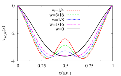
Figure 4: Exact ensemble XC potentials of the 1D box with two electrons. The ensemble contains the ground state and the first (triplet) excited state.

VI.2 Charge-transfer excitation with 1D box

Charge-transfer (CT) excitations are difficult to treat with approximate TDDFT, due to the lack of overlap between orbitals.FRM11 With common approximations, the excitation energy calculated by TDDFT is much smaller than experimental values.U12 Here we provide a 1D example of an excited state with CT character, showing that there is no fundamental difficulty in treating CT excitations with EDFT. Since EDFT calculations do not involve transition densities, they do not suffer from the lack-of-orbital-overlap problem in TDDFT.

The external potential for the CT box is

$$v(x)=\left\{\begin{array}[]{ll}0&x\in[0,1]\cup[2,4]\\ 20&x\in(1,2)\\ \infty&x<0\text{ or }x>4,\end{array}\right.$$ (79)

with the barrier dimensions chosen for numerical stability of the inversion process. The lowest two eigenstate densities are given in the top of Fig. 5. The ground-state and first-excited-state total and kinetic energies of the CT system described are

$$\begin{split}E_{0}&=138.254\,\text{eV},\quad T_{0}=63.4617\,\text{eV (singlet)},\\ E_{1}&=140.652\,\text{eV},\quad T_{1}=112.141\,\text{eV (triplet)}.\end{split}$$ (80)

This significant increase in kinetic energy together with a small total energy change designate the CT character of the first excited state. The electrons become distributed between the two wells of the potential, instead of being confined in one well.

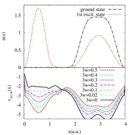
Figure 5: Exact densities and ensemble xc potentials of the 1D charge-transfer box.

The ground- and first-excited-state densities and ensemble XC potentials are plotted in Fig. 5. The potentials show the characteristic step-like structures of charge-transfer excitations, which align the chemical potentials of the two wells.HG12 ; HG13 Table 4 lists the ensemble energies of the CT box. Excitation energies have larger errors than those for the 1D flat box due to greater numerical instability, but they are still accurate to within $0.01$ eV.

$3\texttt{w}$	0.5	0.1	0.02
$E_{1,\texttt{w}}^{\text{KS}}-E_{0,\texttt{w}}^{\text{KS}}$	2.2048	2.4092	2.4317
$\partial E_{{\scriptscriptstyle\rm XC},\texttt{w}}[n]/\partial n|_{n=n_{\texttt{w}}}/3$	0.1993	-0.0108	-0.0334
$\omega_{1,\texttt{w}}$	2.4042	2.3983	2.3983

Table 4: First excitation energy and energy decomposition of the two-multiplet ensemble of the 1D charge-transfer box at different w values, calculated using Eq. (14). All energies are in eV. The exact first excitation energy is $E_{1}-E_{0}=2.3983$ eV. See Supplemental Material for additional data.

VI.3 Hooke’s atom

Hooke’s atom is a popular model systemLaufer1986 ; Filippi1994 with the following external potential:

$$v({\bf r})=\frac{k}{2}\left|{\bf r}\right|^{2}.$$ (81)

For our calculation, $k=1/4$. Though the first excited state has cylindrical symmetry, we use a spherical grid, as it has been shown that the error due to spherical averaging is small.KP87 As a closed-shell system, the spatial parts, and therefore the densities, of the spin-up and spin-down ensemble KS orbitals have to be the same, so we treat this system as a bi-ensemble.

The magnitude of the external potential of the Hooke’s atom is smallest at $r=0$, and becomes larger as $r$ increases. This is completely different from the Coulomb potential of real atoms. Since the electron-electron interaction is still coulombic, $v_{\scriptscriptstyle\rm XC}({\bf r})$ can be expected to have a $-1/r$ behavior as $r\to\infty$, which is negligibly small compared to $v({\bf r})$. Combined with a density that decays faster than real atomic densities, $n({\bf r})\sim\exp(-ar^{2})$ versus $n({\bf r})\sim\exp(-br)$, convergence of the Hooke’s atom $v_{\scriptscriptstyle\rm XC}({\bf r})$ is difficult in the asymptotic region. Additionally, $v_{\scriptscriptstyle\rm XC}({\bf r})\gg v({\bf r})$ for small $r$, so larger discretization errors in this region also contribute to poorer inversion performance. Despite these challenges, we still obtain highly accurate excitation energies.

A logarithmic grid with 550 points ranging from $r=10^{-5}\,\text{a.u.}$ to $10\,\text{a.u.}$ is used for all the Hooke’s atom calculations. On this grid, the exact ground- and first excited-state energies are

$$E_{1}=54.42\,\text{eV},\quad E_{2}=64.19\,\text{eV}.$$ (82)

Calculated $\omega_{2}$ was 9.786 eV for all values of w tested (see Supplemental Material). Unlike the He atom and the 1D flat box, the $n_{\texttt{w}}({\bf r})$ and $v_{{\scriptscriptstyle\rm XC},\texttt{w}}({\bf r})$ show little variation with w (see Supplemental Material). The second KS orbital of the Hooke’s atom is a $p$-type orbital, which has no radial node and a radial shape similar to that of the first KS orbital. Consequently, the changes in the KS and xc potentials are also smaller.

VI.4 He

Using the methods in Ref. YTPB14, , we employ a Hylleraas expansion of the many-body wavefunctiondrake_94 to calculate highly accurate densities of the first few states of the He atom. We report the exact ensemble XC potentials for He singlet ensemble in that paper. Table 5 shows accurate excitation energies calculated from mixed symmetry, three-multiplet, and strictly triplet ensembles, demonstrating the versatility of EDFT.

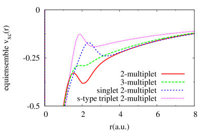
Figure 6: Ensemble XC potentials of the singlet-triplet, singlet-triplet-singlet, strictly singlet, and strictly triplet He equiensembles.

Fig. 6 compares $v_{{\scriptscriptstyle\rm XC},\texttt{w}}({\bf r})$ for four types of He equiensembles, highlighting their different features. The characteristic bump up in these potentials is shifted left in the 2-multiplet case, relative to the others shown. This shift has little impact on the first “shell” of the ensemble density’s shell-like structure, but the second is shifted left and has sharper decay, noticeably different from that of the singlet ensemble.YTPB14

2-multiplet ensemble: $\omega_{1}=19.8231$ eV
$\texttt{w}_{2}$	0.25	0.125	0.03125
$E_{1,\texttt{w}_{2}}^{\text{KS}}-E_{0,\texttt{w}_{2}}^{\text{KS}}$	25.1035	22.4676	21.6502
$\partial E_{\scriptscriptstyle\rm{xc},\texttt{w}_{2}}[n]/\partial\texttt{w}_{2}|_{n=n_{\texttt{w}_{2}}}$	-15.8099	-7.9358	-5.4351
$(E_{1}-E_{0})_{\texttt{w}_{2}}$	19.8336	19.8224	19.8385
3-multiplet ensemble: $\omega_{2}=20.6191$ eV
$\texttt{w}_{3}$	0.2	0.1	0.025
$E_{2,\texttt{w}_{3}}^{\text{KS}}-E_{0,\texttt{w}_{3}}^{\text{KS}}$	26.8457	25.8895	25.2853
$\partial E_{\scriptscriptstyle\rm{xc},\texttt{w}_{3}}[n]/\partial\texttt{w}_{3}|_{n=n_{\texttt{w}_{3}}}$	-0.9596	-0.7207	-0.5696
$(E_{2}-E_{0})_{\texttt{w}_{2},\texttt{w}_{3}}$	20.6270	20.6184	20.6306
triplet ensemble: $\omega_{1}=2.8991$ eV
w	0.16667	0.08333	0.02083
$E_{1}^{\text{KS}}-E_{0}^{\text{KS}}$	2.8928	2.8956	2.8967
$\partial E_{{\scriptscriptstyle\rm XC},\texttt{w}}[n]/\partial\texttt{w}|_{n=n_{\texttt{w}}}$	0.0187	0.0104	0.0074
$(E_{1}-E_{0})_{\texttt{w}}$	2.8990	2.8990	2.8992

Table 5: He atom excitation energies, calculated using Eq. (14) and various ensemble types: singlet-triplet (2-multiplet), singlet-triplet-singlet (3-multiplet), and strictly triplet. All energies are in eV. $\texttt{w}_{2}$ dependency of the 3-multiplet excitation energies is noted explicitly, though $\texttt{w}_{2}=(1-\texttt{w}_{3})/4$ for the GOK ensemble. See Supplemental Material for additional data and figures.

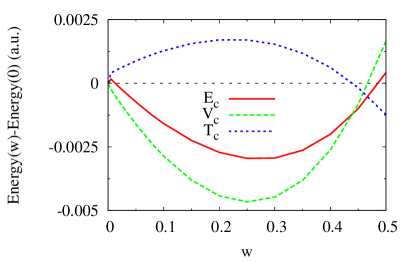
Figure 7: Behaviors of the various energy components for the singlet ensemble of He. The ground state ($\texttt{w}=0$) values are taken from Ref. HU97, . The small kinks near $\texttt{w}=0$ are due to the difference in the numerical approaches of this work and Ref. HU97, .

The inequalities shown in Sec. IV.1 and the virial theorem Eq. (64) are verified by the exact results. Behaviors of the energy components for the singlet ensemble versus w are plotted in Fig. 7. Correlation energies show strong non-linear behavior in w. According to Eq. (14), the excitation energies are related to the derivative of $E_{\scriptscriptstyle\rm XC}$ versus w. Therefore, $E_{\scriptscriptstyle\rm C}$ is crucial for accurate excitation energies, even though its absolute magnitude is small.

VII Conclusion

This paper is an in-depth exploration of ensemble DFT, an alternative to TDDFT for extracting excitations from DFT methodology. Unlike TDDFT, EDFT is based on a variational principle, and so one can expect that the failures and successes of approximate functionals should occur in different systems than those of TDDFT.

Apart from exploring the formalism and showing several new results, the main result of this work is to apply a new algorithm to highly-accurate densities of eigenstates to explore the exact EDFT XC potential. We find intriguing characteristic features of the exact potentials that can be compared against the performance of old and new approximations. We also extract the weight-dependence of the KS eigenvalues, which are needed to extract accurate transition frequencies, and find that a large cancellation of weight-dependence occurs in the exact ensemble. Many details of these calculations are reported in the supplemental information.

From the original works of Gross, Oliviera, and Kohn, ensemble DFT has been slowly developed over three decades by a few brave pioneering groups, most prominently that of Nagy. We hope that the insight these exact results bring will lead to a plethora of new ensemble approximations and calculations and, just possibly, a competitive method to treating excitations within DFT.

References

- [1] P. Hohenberg and W. Kohn. Inhomogeneous electron gas. Phys. Rev., 136:B864, 1964.
- [2] W. Kohn and L. J. Sham. Self-consistent equations including exchange and correlation effects. Phys. Rev., 140:A1133, 1965.
- [3] K. Burke. Perspective on density functional theory. J. Chem. Phys., 136, 2012.
- [4] E. Runge and E. K. U. Gross. Density-functional theory for time-dependent systems. Phys. Rev. Lett., 52:997, 1984.
- [5] M. E. Casida. Time-dependent density functional response theory of molecular systems: theory, computational methods, and functionals. In J. M. Seminario, editor, Recent developments and applications in density functional theory. Elsevier, Amsterdam, 1996.
- [6] M. A. L. Marques, N. T. Maitra, F. M. S. Nogueira, E. K. U. Gross, and A. Rubio, editors. Fundamentals of Time-Dependent Density Functional Theory. Lecture Notes in Physics. Springer, Berlin, 2012.
- [7] C. A. Ullrich. Time-Dependent Density-Functional Theory: Concepts and Applications. Oxford University Press, Oxford, 2012.
- [8] Giovanni Onida, Lucia Reining, and Angel Rubio. Electronic excitations: density-functional versus many-body green’s-function approaches. Rev. Mod. Phys., 74(2):601–659, Jun 2002.
- [9] Neepa T. Maitra, Fan Zhang, Robert J. Cave, and Kieron Burke. Double excitations within time-dependent density functional theory linear response. The Journal of Chemical Physics, 120(13):5932–5937, 2004.
- [10] Miquel Huix-Rotllant, Andrei Ipatov, Angel Rubio, and Mark E. Casida. Assessment of dressed time-dependent density-functional theory for the low-lying valence states of 28 organic chromophores. Chemical Physics, 391(1):120 – 129, 2011.
- [11] C. A. Ullrich and Z.-H. Yang. A brief compendium of time-dependent density-functional theory. Brazilian J. Phys., 44:154, 2014.
- [12] Peter Elliott, Sharma Goldson, Chris Canahui, and Neepa T. Maitra. Perspectives on double-excitations in TDDFT. Chemical Physics, 391(1):110 – 119, 2011.
- [13] J. L. Weisman A. Dreuw and M. Head-Gordon. Long-range charge-transfer excited states in time-dependent density functional theory require non-local exchange. J. Chem. Phys., 119:2943, 2003.
- [14] D.J. Tozer. Relationship between long-range charge-transfer excitation energy error and integer discontinuity in Kohn-Sham theory. J. Chem. Phys., 119:12697, 2003.
- [15] A. Görling. Density-functional theory for excited states. Phys. Rev. A, 54:3912, 1996.
- [16] I. Frank, J. Hutter, D. Marx, and M. Parrinello. Molecular dynamics in low-spin excited states. The Journal of Chemical Physics, 108(10):4060–4069, 1998.
- [17] M. Levy and Á. Nagy. Variational density functional theory for an individual excited state. Phys. Rev. Lett., 83:4361, 1999.
- [18] A.K. Theophilou. The energy density functional formalism for excited states. J. Phys. C, 12:5419, 1979.
- [19] E. K. U. Gross, L. N. Oliveira, and W. Kohn. Rayleigh-Ritz variational principle for ensemble of fractionally occupied states. Phys. Rev. A, 37:2805, 1988.
- [20] E. K. U. Gross, L. N. Oliveira, and W. Kohn. Density-functional theory for ensembles of fractionally occupied states. I. Basic formalism. Phys. Rev. A, 37:2809, 1988.
- [21] L. N. Oliveira, E. K. U. Gross, and W. Kohn. Density-functional theory for ensembles of fractionally occupied states. II. Application to the He atom. Phys. Rev. A, 37:2821, 1988.
- [22] Á. Nagy. Exact ensemble exchange potentials for multiplets. Int. J. Quantum Chem., 56(S29):297–301, 1995.
- [23] Á Nagy. Optimized potential method for ensembles of excited states. Int. J. Quant. Chem., 69:247, 1998.
- [24] R. Singh and B. M. Deb. Developments in excited-state density functional theory. Phys. Rep., 311:47, 1999.
- [25] Á Nagy. An alternative optimized potential method for ensembles of excited states. Journal of Physics B: Atomic, Molecular and Optical Physics, 34(12):2363, 2001.
- [26] O. Franck and E. Fromager. Generalised adiabatic connection in ensemble density-functional theory for excited states: example of the H2 molecule. Molecular Physics, pages 1–18, 2013.
- [27] A. D. Becke. Density-functional exchange-energy approximation with correct asymptotic behavior. Phys. Rev. A, 38(6):3098–3100, Sep 1988.
- [28] C. Lee, W. Yang, and R. G. Parr. Development of the Colle-Salvetti correlation-energy formula into a functional of the electron density. Phys. Rev. B, 37(2):785–789, Jan 1988.
- [29] A. D. Becke. Density-functional thermochemistry. III. The role of exact exchange. The Journal of Chemical Physics, 98(7):5648–5652, 1993.
- [30] J. P. Perdew, K. Burke, and M. Ernzerhof. Generalized gradient approximation made simple. Phys. Rev. Lett., 77(18):3865–3868, Oct 1996. ibid. 78, 1396(E) (1997).
- [31] K. Burke J.P. Perdew and M. Ernzerhof. Perdew, Burke, and Ernzerhof Reply. Phys. Rev. Lett., 80:891, 1998.
- [32] Denis Jacquemin, Valérie Wathelet, Eric A. Perpète, and Carlo Adamo. Extensive TD-DFT benchmark: Singlet-excited states of organic molecules. Journal of Chemical Theory and Computation, 5(9):2420–2435, 2009.
- [33] N. I. Gidopoulos, P. G. Papaconstantinou, and E. K. U. Gross. Spurious interactions, and their correction, in the ensemble-Kohn-Sham scheme for excited states. Phys. Rev. Lett., 88:033003, 2002.
- [34] F Tasnádi and Á Nagy. Ghost- and self-interaction-free ensemble calculations with local exchange-correlation potential for atoms. Journal of Physics B: Atomic, Molecular and Optical Physics, 36(20):4073, 2003.
- [35] F. Tasnádi and Á. Nagy. An approximation to the ensemble Kohn-Sham exchange potential for excited states of atoms. The Journal of Chemical Physics, 119(8):4141–4147, 2003.
- [36] Z.-H. Yang, , J. R. Trail, A. Pribram-Jones, K. Burke, R. J. Needs, and C. Ullrich. Exact ensemble density-functional theory for excited states. arxiv: 1402.3209, submitted to Phys. Rev. Lett., 2014.
- [37] M. Levy and J.P. Perdew. Hellmann-Feynman, virial, and scaling requisites for the exact universal density functionals. shape of the correlation potential and diamagnetic susceptibility for atoms. Phys. Rev. A, 32:2010, 1985.
- [38] C. Filippi, C. J. Umrigar, and M. Taut. Comparison of exact and approximate density functionals for an exactly soluble model. The Journal of Chemical Physics, 100(2):1290–1296, 1994.
- [39] Paul Hessler, Neepa T. Maitra, and Kieron Burke. Correlation in time-dependent density-functional theory. The Journal of Chemical Physics, 117(1):72–81, 2002.
- [40] M Levy. Excitation energies from density-functional orbital energies. Phys. Rev. A, 52:R4313, 1995.
- [41] There appears to be a sign error in Eq. (16) of Ref. 40: the two terms on the right-hand side should be swapped.
- [42] R. M. Dreizler and E. K. U. Gross. Density Functional Theory: An Approach to the Quantum Many-Body Problem. Springer–Verlag, Berlin, 1990.
- [43] W. Kohn. Density-functional theory for excited states in a quasi-local-density approximation. Phys. Rev. A, 34:737, 1986.
- [44] E.H. Lieb and B. Simon. Thomas-Fermi theory revisited. Phys. Rev. Lett., 31:681, 1973.
- [45] John P. Perdew, Adrienn Ruzsinszky, Lucian A. Constantin, Jianwei Sun, and Gabor I. Csonka. Some fundamental issues in ground-state density functional theory: A guide for the perplexed. Journal Of Chemical Theory and Computation, 5(4):902–908, Apr 2009.
- [46] R.T. Sharp and G.K. Horton. A variational approach to the unipotential many-electron problem. Phys. Rev., 90:317, 1953.
- [47] J.D. Talman and W.F. Shadwick. Optimized effective atomic central potential. Phys. Rev. A, 14:36, 1976.
- [48] J.B. Krieger, Y. Li, and G.J. Iafrate. Phys. Lett. A, 146:256, 1990.
- [49] O. Gunnarsson and B. I. Lundqvist. Exchange and correlation in atoms, molecules, and solids by the spin-density-functional formalism. Phys. Rev. B, 13:4274, 1976.
- [50] A. Görling. Symmetry in density-functional theory. Phys. Rev. A, 47:2783, 1993.
- [51] R. G. Parr and W. Yang. Density Functional Theory of Atoms and Molecules. Oxford University Press, 1989.
- [52] K. Burke, F. G. Cruz, and K.-C. Lam. Unambiguous exchange-correlation energy density for hooke’s atom. Int. J. Quant. Chem., 70:583, 1998.
- [53] John P. Perdew and Yue Wang. Accurate and simple analytic representation of the electron-gas correlation energy. Phys. Rev. B, 45(23):13244–13249, Jun 1992.
- [54] Johanna I. Fuks, Angel Rubio, and Neepa T. Maitra. Charge transfer in time-dependent density-functional theory via spin-symmetry breaking. Phys. Rev. A, 83:042501, Apr 2011.
- [55] M. Hellgren and E. K. U. Gross. Discontinuities of the exchange-correlation kernel and charge-transfer excitations in time-dependent density-functional theory. Phys. Rev. A, 85:022514, Feb 2012.
- [56] Maria Hellgren and E. K. U. Gross. Discontinuous functional for linear-response time-dependent density-functional theory: The exact-exchange kernel and approximate forms. Phys. Rev. A, 88:052507, 2013.
- [57] P. M. Laufer and J. B. Krieger. Test of density-functional approximations in an exactly soluble model. Phys. Rev. A, 33:1480, 1986.
- [58] C. Filippi, C. J. Umrigar, and M. Taut. Comparison of exact and approximate density functionals for an exactly soluble model. J. Chem. Phys., 100:1290, 1994.
- [59] F. W. Kutzler and G. S. Painter. Energies of atoms with nonspherical charge densities calculated with nonlocal density-functional theory. Phys. Rev. Lett., 59:1285, 1987.
- [60] G. W. F. Drake and Z.-C. Yan. Variational eigenvalues for the S states of helium. Chem. Phys. Lett., 229:486, 1994.
- [61] C.-J. Huang and C. J. Umrigar. Local correlation energies of two-electron atoms and model systems. Phys. Rev. A, 56:290, 1997.
- [62] See supplemental material at [URL will be inserted by AIP] for discretization details, additional figures, and extended data tables.