A Numerical Assessment of Cosmic-ray Energy Diffusion through Turbulent Media

Abstract

How and where cosmic rays are produced, and how they diffuse through various turbulent media, represent fundamental problems in astrophysics with far reaching implications, both in terms of our theoretical understanding of high-energy processes in the Milky Way and beyond, and the successful interpretation of space-based and ground based GeV and TeV observations. For example, recent and ongoing detections, e.g., by Fermi (in space) and HESS (in Namibia), of $\gamma$-rays produced in regions of dense molecular gas hold important clues for both processes. In this paper, we carry out a comprehensive numerical investigation of relativistic particle acceleration and transport through turbulent magnetized environments in order to derive broadly useful scaling laws for the energy diffusion coefficients.

1 Introduction

Until recently, the widely held paradigm for the origin of cosmic rays, at least below the knee at roughly $1$ PeV, promoted the view that all of the intragalactic injection occurred via first-order Fermi acceleration in supernova shells. But any direct evidence for this view is meager and equivocal. More recently, data from balloon-borne experiments have refuted the expectation from supernova acceleration schemes that the cosmic-ray spectrum ought to be structureless and universal (Wefel 1988). The latest measurements with PAMELA confirm and extend the balloon-based claims (Adriani et al. 2011). These data seem to call for a diverse variety of acceleration sites and mechanisms throughout the Galaxy.

In recent work (Fatuzzo & Melia 2011, 2012a, 2012b), we have begun to assess the feasibility of stochastic acceleration within turbulent magnetized regions using highly detailed simulations of individual particle trajectories. A principal goal of this work is to accurately determine the spatial and energy diffusion coefficients of cosmic-ray protons in a broad range of environments, e.g., inside molecular clouds and the more tenuous intercloud medium. The spatial and energy diffusion coefficients calculated over a broad range of parameter space may be used, e.g., to compare estimates of the time required to energize protons up to TeV energies with the escape and cooling times throughout the interstellar medium. In previous applications, this approach has allowed us to conclude that protons in the intercloud medium at the galacitc center can be energized up to the $1-10$ TeV energies required to account for the observed HESS emission in this region (Aharonian et al. 2006; Liu et al. 2006a; Ballantyne et al. 2007; Wommer et al. 2008; see also Markoff et al. 1997, 1999; Liu & Melia 2001). Stochastic particle acceleration by magnetic turbulence appears to be a viable mechanism for cosmic-ray production at the galactic center (Liu et al. 2006b).

Developing an understanding of how the spatial diffusion coefficients depend on the physical environment and energy of the particles was the subject of our previous work (Fatuzzo et al. 2010, 2011). The focus of the present paper is specifically to determine the diffusion of cosmic rays in energy space, with its attendant dependence on all of the critical physical characteristics of the medium, such as the magnetic intensity, degree of turbulence, and size of the fluctuations. As before, we do this by using a modified numerically based formalism developed for the general study of cosmic-ray diffusion by Giacalone & Jokipii (1994). This approach has already been used successfully in several other contexts (see, e.g., O’Sullivan et al 2009; Fatuzzo & Melia 2012a, 2012b). Here, we will extend this robust numerically-based framework for the general analysis of stochastic acceleration of cosmic-rays by the turbulent electric fields generated along with the time-dependent turbulent magnetic field in a dynamically active medium.

We stress that our adopted model of turbulence as a superposition of Alfvénic like waves with linear dispersion relations is not meant to fully describe MHD turbulence in the interstellar medium (ISM). For example, the model does not account for the fact that magnetic fluctuations decorrelate due to non-linear interactions before they can propagate over distances of multiple wavelengths (Goldreich & Sridhar 1995) – an effect that leads to resonance broadening and as such, influences how thermal particles interact with turbulence (Lynn et al. 2012; 2013). However, our intent is to adopt a formalism that adequately describes turbulence as seen locally by highly relativistic cosmic rays. Since relativistic particles have speeds that are much greater than the Alfvén speeds considered in our analysis (which is then the limit in which our results are expected to be valid), they should not be sensitive to dynamical processes that occur on MHD timescales. In essence, we are relying on basic principles (e.g., the scaling laws between intensity and wavelength) to capture the global features of MHD turbulence that affect the propagation and acceleration of high energy cosmic rays.

The work presented here extends the results of previous works, most notably, that of O’Sullivan et al. (2012), as it significantly broadens the explored parameter space and also considers anisotropically distributed wave vectors (Goldreich & Sridhar 1995; Cho & Vishniac 2000). We focus primarily on strong turbulence ($\delta B\sim B$) for which quasilinear theory is not applicable, although we do present results for isotropic weak turbulence as a consistency check. Our paper is organized as follows. The pertinent properties of the medium through which the particles diffuse are outlined in §2. The scheme for generating the turbulent magnetic and electric fields is presented in §3, along with the equations that govern the motion of cosmic rays. The basic elements of stochastic acceleration are discussed in §4, and the results of our work are presented in §5. The conclusions of our work are summarized in §6.

2 The Physical Medium

The physical parameters found throughout the intergalactic and interstellar media have values that span several orders of magnitude. Of particular interest to our study, the most vacuous regions of the intergalactic medium have particle number densities $n\lower 2.15277pt\hbox{$\;\buildrel<\over{\sim}\;$}10^{-3}$ cm^-3 and magnetic field strengths $B\lower 2.15277pt\hbox{$\;\buildrel<\over{\sim}\;$}0.1\mu$G (see, e.g., Kronberg 1994; Fraschetti & Melia 2008). In contrast, the denser regions near the supermassive black hole at the galactic center have densities $n\gtrsim 10^{12}$ cm^-3 and field strengths $B\gtrsim 1$ G (Ruffert & Melia 1994; Falcke & Melia 1997; Kowalenko & Melia 1999; Melia 2007; see also Misra & Melia 1993 for the case of stellar-mass size black holes).

Exactly how the magnetic field is partitioned within these various media is not yet known, but there is a general relation between density and field strength. In the simplest case where flux freezing applies (say in the ISM), the magnetic field strength $B$ would scale with gas density $n$ according to $B\propto n^{1/2}$. It is noteworthy, then, that an analysis of magnetic field strengths measured in molecular clouds yields a relation between $B$ and $n$ of the form

$$B\sim 10\,\mu\hbox{\rm G}\left({n\over 10^{2}\,\hbox{\rm cm}^{-3}}\right)^{0.47}\;,$$ (1)

though with a significant amount of scatter in the data used to produce this fit (Crutcher 1999; see also Fatuzzo et al. 2006 and references cited therein). This result is consistent with the idea that nonthermal linewidths, measured to be $\sim$$1$ km s^-1 throughout the cloud environment (e.g., Lada et al. 1991), arise from MHD fluctuations.

Of course, even among molecular clouds, the physical environment can be quite different depending on location. Near the galactic center, the molecular clouds are considerably different from their counterparts in the disk. For example, the average molecular hydrogen number density over the Sgr B complex—the largest molecular cloud complex (Lis & Goldsmith 1989; Lis & Goldsmith 1990; Paglione et al. 1998) near the galactic center—has a density $3$–$10\times 10^{3}$ cm^-3. Like its traditional counterparts, Sgr B displays a highly nonlinear structure, containing two bright sub-regions, Sgr B1 and Sgr B2, the latter having an average molecular density of $\sim 10^{6}$ cm^-3, and containing three dense ($n\sim 10^{7.3-8}$ cm^-3), small ($r\sim 0.1$ pc) cores—labeled North, Main and South. These cores also show considerable structure, containing numerous ultra-compact and hyper-compact HII regions. As such, the densities associated with the galactic-center molecular clouds are about two orders of magnitude greater than those in the disk of our galaxy.

The exact nature of magnetic turbulence in these environments is itself not well constrained, though magnetic fluctuations typically have a power-law spectrum. Their intensity at a given wavelength scales according to $(\delta B_{\lambda})^{2}\sim\lambda^{\Gamma-1}$, with values of $\Gamma=1$ (Bohm), $\Gamma=3/2$ (Kraichnan) or $\Gamma=5/3$ (Kolmogorov) often adopted. In addition, the range in wavelengths over which these fluctuations occurs is not well known, though it is reasonable to assume that the upper end corresponds to the lengthscale over which the fluctuations are generated. (For example, in the ISM, the turbulence is generated by supernova remnants and stellar-wind collisions, so one might expect the longest wavelength to be on the order of several parsecs or less; see, e.g., Coker & Melia 1997; Melia & Coker 1999.) The lower end must be smaller than the characteristic length scale associated with the particle motion (i.e., the gyration radius), under the assumption that magnetic energy ultimately dissipates into plasma energy via its coupling to these particles.

3 Governing Equations

We explore how cosmic rays diffuse through a homogeneous hydrogen gas of mass density $\rho=nm_{p}$ threaded by a uniform static background field ${\bf B_{0}}$, on which magnetic and electric fluctuations propagate. From our numerical simulations, we then compute energy diffusion coefficients covering a broad range of particle energies and parameter space expected to span the great diversity of environments observed both within our galaxy and in the intergalactic medium. We focus primarily on strong turbulence, for which the energy density of the turbulent fields is comparable to that of the background fields.

A standard numerical approach to studying cosmic-ray diffusion treats the spatially fluctuating magnetic component $\delta{\bf B}$ as the superposition of a large number of randomly polarized transverse waves with wavelengths $\lambda_{n}=2\pi/k_{n}$, logarithmically spaced between $\lambda_{min}$ and $\lambda_{max}$ (e.g., Giancoli & Jokipii 1994; Casse et al. 2002; Fatuzzo et al. 2010). Adopting a static turbulent field removes the necessity of specifying a dispersion relation between the wavevectors $k_{n}$ and their corresponding angular frequencies $\omega_{n}$. This approach appears suitable for considering highly non-linear turbulence ($\delta B>>B_{0}$), or simply an environment without a background component. Of course, turbulent magnetic fields in cosmic environments are not static. Nevertheless, a static formalism in spatial diffusion calculations of relativistic particles seems justified for environments in which the Alfvén speed is much smaller than the speed of light.

The situation in this paper is quite different: we are focusing on the energy diffusion of cosmic rays propagating through a turbulent magnetic field, which requires the use of a time-dependent formalism in order to self-consistently include the fluctuating electric fields that must also be present (say, from Faraday’s law). At present, such a theory of MHD turbulence in the interstellar medium remains elusive. Nevertheless, it is generally understood that turbulence is driven from a cascade of longer wavelengths to shorter wavelengths as a result of wave-wave interactions. For strong MHD turbulence in a uniform medium, this cascade seemingly produces eddies on small spatial scales that are elongated in the direction of the underlying magnetic field, so that the components of the wave vector along ($k_{||}$) and across ($k_{\perp}$) the underlying field direction are related by the expression $k_{||}\propto k_{\perp}^{2/3}$, with a Kolmogorov energy spectrum that scales as $k_{\perp}^{-5/3}$ (Goldreich & Sridhar 1995; Cho & Lazarian 2003).

It is beyond the scope of this paper to develop a self-consistent theory of MHD turbulence in the ISM that includes electric field fluctuation. We therefore adopt the formalism of O’Sullivan et al (2012). Specifically, we assume a medium represented by a nonviscous, perfectly conducting fluid threaded by a uniform static field ${\bf B_{0}}$, and use linear MHD theory as a guide. In the linear regime, one can encounter three types of MHD waves: Alfvén, fast and slow. As in O’Sullivan et al. (2009), we here consider only Alfvén waves, for which the turbulent magnetic field may be written as a sum of $N$ randomly directed waves

$$\delta{\bf B}=\sum_{n=1}^{N}{\bf A_{n}}\,e^{i({\bf k_{n}}\cdot{\bf r}-\omega_{n}t+\beta_{n})}\,.$$ (2)

As noted already, this formalism does not adequately describe decorrelation effects known to be important for thermal cosmic rays (Lynn et al. 2012; 2013). But it should serve as a reasonable model for the turbulence experienced by particles with velocities much greater than the Alfvén speed $v_{A}$, as such particles would be expected to travel over many correlation lengths ($\sim 0.1\lambda_{max}$) in an Alfvén time $\tau_{A}\sim\lambda_{max}/v_{A}$.

To keep the analysis as broad as possible, we focus on an isotropic turbulence spectrum, but we also perform a suite of experiments with anisotropic turbulence as informed by the results of Golreich & Sridhar (1995). For the isotropic case, the direction of each propagation vector ${\bf k_{n}}$ is set through a random choice of polar angles $\theta_{n}$ and $\phi_{n}$, and the phase of each term is set through a random choice of $\beta_{n}$. The sum has $N=N_{k}\log_{10}[k_{max}/k_{min}]$ terms, with $k_{n}$ evenly spaced on a logarithmic scale between $k_{min}=2\pi/\lambda_{max}$ and $k_{max}=2\pi/\lambda_{min}$. A value of $N_{k}$ = 25 appears to provide enough terms to suitably model what is really a continuous rather than a discrete system. The appropriate choice of $\Gamma$ in the scaling

$$A_{n}^{2}=A_{1}^{2}\left[{k_{n}\over k_{1}}\right]^{-\Gamma}{\Delta k_{n}\over\Delta k_{1}}=A_{1}^{2}\left[{k_{n}\over k_{1}}\right]^{-\Gamma+1}$$ (3)

sets the desired spectrum of magnetic turbulence (e.g., $\Gamma=3/2$ for Kraichnan and 5/3 for Kolmogorov turbulence). For our adopted scheme, the value of $\Delta k_{n}/k_{n}$ is the same for all $n$. The normalization for $A_{1}$ is set by the parameter

$$\eta={\langle\delta B^{2}\rangle\over B_{0}^{2}}\;,$$ (4)

defined as the ratio of magnetic energy density in the turbulent component to that of the static background field $B_{0}$.

For the anisotropic case, the direction of each perpendicular wavevector $k_{n\perp}$ is set through a random choice of azimuthal angle $\phi_{n}$, and the phase of each term is again set through a random choice of $\beta_{n}$. The corresponding parallel component of the wavevector is then set through the relation

$$k_{n||}=\pm{\sqrt{2}\over 2}k_{1\perp}^{1/3}\,k_{n\perp}^{2/3}\,$$ (5)

(with a randomly chosen sign), such that

$$k_{1}=\sqrt{k_{1\perp}^{2}+k_{1||}^{2}}={2\pi\over\lambda_{max}}\;.$$ (6)

Consistent with the results of Goldreich & Sridhar (1995), we only consider a Kolmogorov profile, so that

$$A_{n}^{2}=A_{1}^{2}\left[{k_{n\perp}\over k_{1\perp}}\right]^{-2/3}\,.$$ (7)

Since Alfvén waves don’t compress the fluid through which they propagate, their fluid velocity ${\bf v}$ satisfies the condition ${\bf k}\cdot{\bf v}=0$. In addition, ${\bf v}\cdot{\bf B_{0}}=0$ for Alfvén waves. The fluid velocity associated with the $n$-th term in Equation (2) is therefore

$$\delta{\bf v_{n}}=\pm A_{n}\,{v_{A}\over B_{0}}\,{{\bf B_{0}}\times{\bf k_{n}}\over|{\bf B_{0}}\times{\bf k_{n}}|}\,e^{i({\bf k_{n}}\cdot{\bf r}-\omega_{n}t+\beta_{n})}\,,$$ (8)

where the sign is chosen randomly for each term in the sum. The dispersion relation for Alfveńic waves is given by the expression

$$\omega_{n}=v_{A}|k_{n\|}|\,.$$ (9)

Each wave has a magnetic field given by the linear form of Ampère’s Law,

$${\bf A_{n}}=\mp A_{n}\,{{\bf k_{n}}\cdot{\bf B_{0}}\over|{\bf k_{n}}\cdot{\bf B_{0}}|}\,{{\bf B_{0}}\times{\bf k_{n}}\over|{\bf B_{0}}\times{\bf k_{n}}|}\,,$$ (10)

which is identical to that of O’Sullivan et al. (2009).

Insofar as the electric fields are concerned, if we were to naively extrapolate from the results of linear MHD theory, the total electric field $\delta{\bf E}$ associated with the turbulent magnetic field in Equation (2) would be given by a sum over the terms

$$\delta{\bf E_{n}}=-\delta{\bf v_{n}}\times{\bf B_{0}}\,.$$ (11)

Notice that $\delta{\bf E}\cdot{\bf B_{0}}$ = 0, but the second order term $\delta{\bf E}\cdot\delta{\bf B}\neq 0$. The presence of an electric field component parallel to the magnetic field in this second order term can significantly increase the acceleration efficiency artificially, especially if the formalism is extended to the nonlinear regime ($\delta B\sim$$B_{0}$). However, the interstellar medium is highly conductive, so any electric field component parallel to the magnetic field should be quickly quenched. O’Sullivan et al. (2009) circumvented this problem by first obtaining the total fluid velocity $\delta{\bf v}$ via the summation

$$\delta{\bf v}=\sum_{n=1}^{N}\delta{\bf v_{n}}\,,$$ (12)

and then using the MHD condition to set the total electric field:

$$\delta{\bf E}=-{\delta{\bf v}\over c}\times{\bf B}\;,$$ (13)

where ${\bf B}={\bf B_{0}}+\delta{\bf B}$. This is the procedure we too will use here.

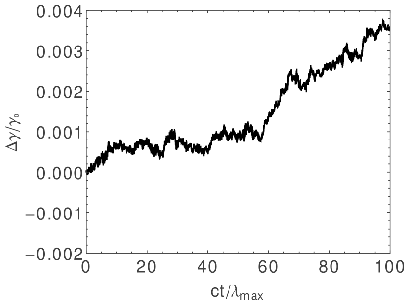
Figure 1: The fractional change in particle energy $\Delta\gamma/\gamma_{0}$ as a function of time for a $\gamma_{0}=10^{5}$ particle injected into an environment ($B_{0}=100\,\mu$G, $n=10^{2}$ cm^-3) with an isotropic Alfvénic turbulent field defined by the parameters $\lambda_{max}=0.1$ pc, $\Gamma=5/3$, and $\eta=1.0$.

With these electric and magnetic field components, one may then solve the Lorentz force equation

$${d\over dt}(\gamma m_{p}{\bf v})=e\left[\delta{\bf E}+{{\bf v}\times{\bf B}\over c}\right]\;,$$ (14)

with

$${d{\bf r}\over dt}=\bf v\;,$$ (15)

to determine the motion of a relativistic charged proton with Lorentz factor $\gamma$ through the turbulent medium. The solutions to these equations are not sensitive to the value of $\lambda_{min}$ so long as the particle’s gyration radius $R_{g}=\gamma mc^{2}/(eB)>>\lambda_{min}$ (Fatuzzo et al. 2010). As such, we set $\lambda_{min}=0.1\gamma mc^{2}/(eB_{0})$ in all our simulations. To completely specify the physical state of an environment to be studied, we must therefore provide values for the parameters $B_{0}$, $n$, $\lambda_{max}$, $\Gamma$ and $\eta$.

4 Basic Elements of Stochastic Acceleration

The motion of a charged particle in perpendicular uniform electric and magnetic fields represents a fundamental topic in electrodynamics and is well understood. It is therefore easy to show that in general, the charge gains and loses kinetic energy in cyclic fashion as it “drifts” in the ${\bf E}\times{\bf B}$ direction.

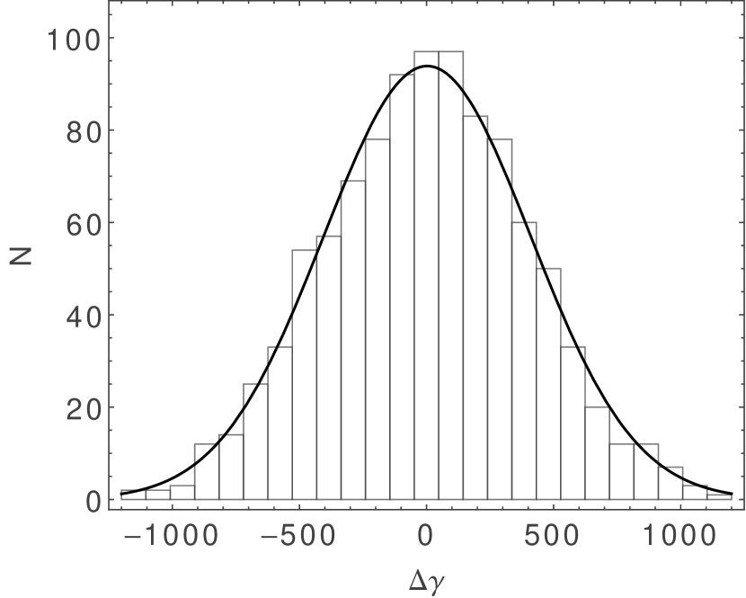
Figure 2: The particle energy distribution at time $t=1000\lambda_{max}/c$ for an ensemble of $N_{p}=1,000$ particles injected into an environment ($B_{0}=100\,\mu$G, $n=10^{2}$ cm^-3) with an anisotropic Alfvénic turbulent field defined by the parameters $\lambda_{max}=0.1$ pc, $\Gamma=5/3$, and $\eta=1.0$. The solid line shows a Gaussian fit to the data.

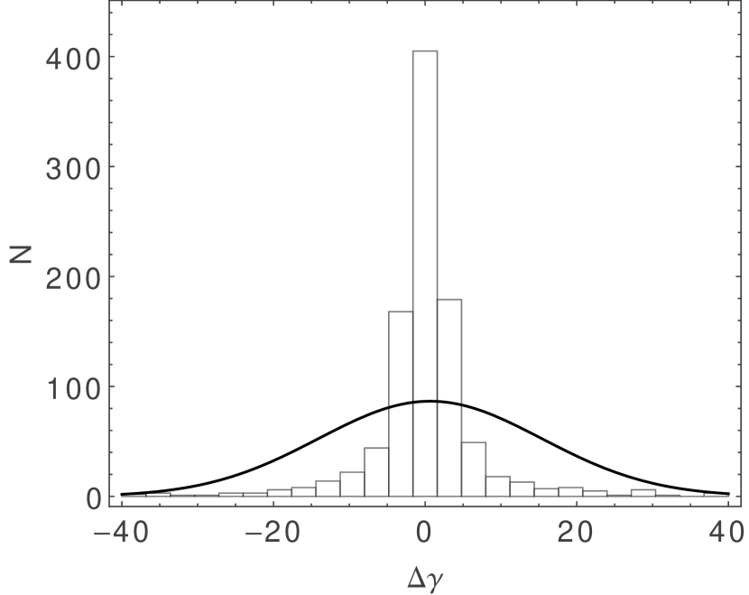
Figure 3: The particle energy distribution at time $t=1000\lambda_{max}/c$ for the ensemble of $N_{p}=1,000$ particles injected into an environment ($B_{0}=100\,\mu$G, $n=10^{2}$ cm^-3) with an anisotropic Alfvénic turbulent field defined by the parameters $\lambda_{max}=0.1$ pc, $\Gamma=5/3$, and $\eta=0.01$. The solid line shows a Gaussian fit to the data.

In the turbulent medium in which the magnetic and electric fields are perpendicular, a single particle’s energy, characterized by $\Delta\gamma/\gamma_{0}=\gamma/\gamma_{0}-1$, therefore exhibits a random-walk like behavior, as shown in figure 1. The energy distribution of an ensemble of particles injected with the same Lorentz factor $\gamma_{0}$ thus broadens as the particles sample the turbulent nature of the accelerating electric fields. Interestingly, these distributions appear Gaussian for all of the isotropic and $\eta=1$ anisotropic cases explored in our analysis. This point is illustrated by figure 2, which shows the distribution of $\Delta\gamma$ values at time $t=1000\lambda_{max}/c$ for an ensemble of $1,000$ particles injected with $\gamma_{0}=10^{5}$ into a medium defined by the same parameters used to calculate the energy evolution shown in figure 1, but with an anisotropic turbulence profile. In such cases, one can therefore quantify the stochastic acceleration of particles in turbulent fields through the dispersion of the resulting distributions of initially mono-energetic particles.

In contrast, the particle distributions obtained for anisotropic, weak turbulence ($\eta\ll 1$) cases have wings that are much broader than a Gaussian distribution, so that their dispersion significantly overestimates the true distribution width. This point is illustrated in figure 3, which shows the distribution of $\Delta\gamma$ values at time $t=1000\lambda_{max}/c$ for an ensemble of $1,000$ particles injected with $\gamma_{0}=10^{5}$ into a medium defined by the same parameters used to calculate the distribution shown in figure 2, but with $\eta=0.01$.

To further compare strong and weak isotropic and anisotropic turbulence, we plot in figure 4 the dispersion $\sigma_{\gamma}\equiv\sqrt{\langle\Delta\gamma^{2}\rangle}$ of the $\Delta\gamma$ distribution as a function of time for the particles used to generate figures 2 and 3 (for which the turbulence was anisotropic) along with their isotropic counterparts. As found throughout our analysis, there is little difference between the isotropic and anisotropic cases when the turbulence is strong ($\eta=1$). However, anisotropic turbulence appears to be significantly less effective at energizing particles than isotropic turbulence when $\eta\ll 1$, in agreement with results obtained in the quasi-linear approximation (Chandran 2000; see also Yan & Lazarian 2002).

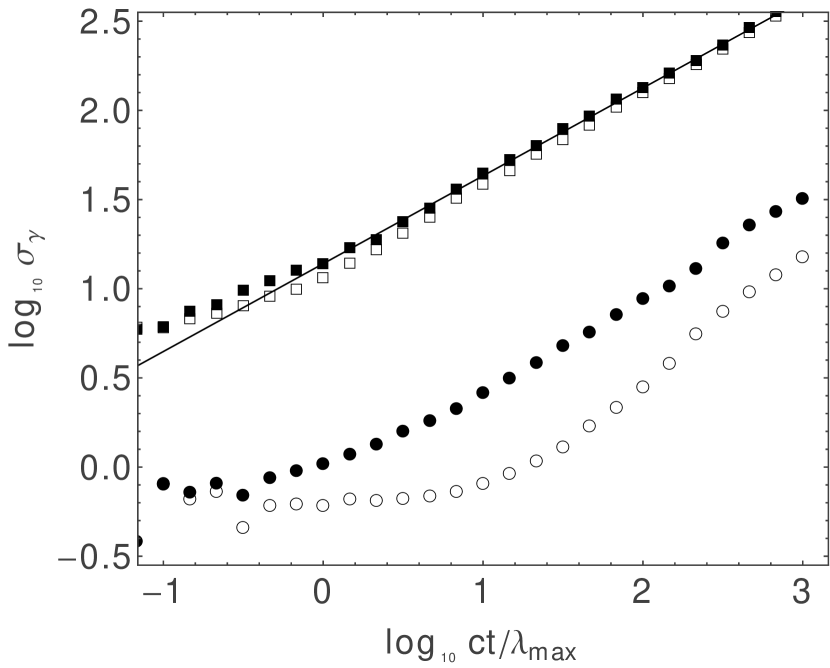
Figure 4: The dispersion of the particle energy distribution as a function of time for the $N_{p}=1,000$ particles injected into an environment ($B_{0}=100\,\mu$G, $n=10^{2}$ cm^-3) with an Alfvénic turbulent field defined by the parameters $\lambda_{max}=0.1$ pc, and $\Gamma=5/3$. Solid squares: isotropic turbulence with $\eta=1.0$. Open squares: anisotropic turbulence with $\eta=1.0$. Solid circles: isotropic turbulence with $\eta=0.01$. Open circles: anisotropic turbulence with $\eta=0.01$. The solid line serves as a reference and has a slope of $1/2$, clearly indicating that $\sigma_{\gamma}\propto\sqrt{t}$ for time $t\gtrsim\lambda_{max}/c$.

Clearly, the chaotic nature of motion through turbulent fields necessitates a statistical analysis. We define a single experiment as a numerical investigation of particle dynamics through a given environment (as defined by the parameters $B_{0}$, $n$, $\Gamma$, $\lambda_{max}$, and $\eta$) over a broad range of particle injection energies (as defined by the Lorentz factor $\gamma_{0}$). As expected from the random nature of stochastic acceleration, $\sigma_{\gamma}\propto\sqrt{t}$ once particles have had a chance to sample the turbulent nature of the underlying electric fields, i.e., for $t\gtrsim\lambda_{max}/c$. This in turn means that the energy diffusion coefficient $D_{\gamma}\equiv\langle\Delta\gamma^{2}\rangle/(2\Delta t)$ can be calculated by using an integration time $\Delta t\gtrsim\lambda_{max}/c$. For each particle energy, we numerically integrate the equations of motion for a time $\Delta t=10\lambda_{max}/c$ for $N_{p}=1,000$ protons randomly injected from the origin. Each particle samples its own unique magnetic field structure (i.e., the values of $\beta_{n}$, $\theta_{n}$, $\phi_{n}$ and the choice of a $\pm$ are chosen randomly for each particle for the isotropic case).

5 Results of Numerical Experiments

We use the procedure described above to carry out a suite of experiments sampling a broad region of parameter space for isotropic turbulence, and perform a limited complimentary set of experiments for anisotropic, strong ($\eta=1$) Kolmogorov turbulence. We limit our analysis to particle energies for which the gyration radius $R_{g}$ falls comfortably below the maximum turbulence wavelength $\lambda_{max}$, so that particles actually diffuse through the turbulent medium. A principal goal of this paper is to determine the relationship between the energy diffusion coefficient $D_{\gamma}$ and the particle’s energy for each experiment. We therefore fit the numerical data using a power law

$$D_{\gamma}=D_{\gamma 0}\gamma^{\alpha}\,.$$ (16)

The parameters for each experiment and corresponding values of $D_{\gamma 0}$ and $\alpha$ obtained through the fits are summarized in Table 1. As a reference, we then compare these empirical fits to the quasi-linear expression

$$D^{ql}_{\gamma}\approx{v_{A}^{2}\over c^{2}}\left({\delta B\over B_{0}}\right)^{2}\left({R_{g}\over\lambda_{max}}\right)^{\Gamma-1}{\gamma^{2}c\over R_{g}}\,,$$ (17)

(Schlickeiser 1989, O’Sullivan et al. 2009). We note that in terms of our parameters, this predicted expression reduces to the simpler form

$$D^{ql}_{\gamma}\propto n^{-1}B_{0}^{4-\Gamma}\eta\,\lambda_{max}^{1-\Gamma}\,\gamma^{\Gamma}\,.$$ (18)

Table 1: Summary of Experiments

Exp	$B_{0}$ ($\mu$G)	$n$ (cm-3)	$\Gamma$	$\lambda_{max}$ (pc)	$\eta$	$D_{\gamma 0}$ (s-1)	$\alpha$
1	100	100	5/3	0.1	1	$5.4\times 10^{-13}$	1.44
2	100	100	5/3	0.1	0.1	$2.5\times 10^{-14}$	1.48
3	100	100	5/3	0.1	0.01	$2.6\times 10^{-16}$	1.63
4	100	100	5/3	0.1	0.001	$5.9\times 10^{-18}$	1.70
5	100	100	3/2	0.1	1	$1.2\times 10^{-12}$	1.39
6	100	100	3/2	0.1	0.001	$2.4\times 10^{-17}$	1.64
7	100	100	1	0.1	1	$6.1\times 10^{-11}$	1.10
8	100	100	1	0.1	0.001	$8.2\times 10^{-15}$	1.20
9	100	1	5/3	0.1	1	$4.7\times 10^{-11}$	1.46
10	100	3.16	5/3	0.1	1	$1.5\times 10^{-11}$	1.46
11	100	10	5/3	0.1	1	$3.9\times 10^{-12}$	1.47
12	100	31.6	5/3	0.1	1	$1.4\times 10^{-12}$	1.46
13	100	316	5/3	0.1	1	$1.2\times 10^{-13}$	1.48
14	100	$10^{3}$	5/3	0.1	1	$5.2\times 10^{-14}$	1.45
15	0.1	100	5/3	0.1	1	$1.1\times 10^{-20}$	1.46
16	3.16	100	5/3	0.1	1	$7.5\times 10^{-17}$	1.45
17	3160	100	5/3	0.1	1	$3.0\times 10^{-9}$	1.46
18	$10^{5}$	100	5/3	0.1	1	$4.0\times 10^{-6}$	1.54
19	100	100	5/3	$10^{-4}$	1	$1.0\times 10^{-11}$	1.48
20	100	100	5/3	100	1	$1.8\times 10^{-14}$	1.47
21	0.1	100	3/2	0.1	1	$1.9\times 10^{-20}$	1.39
22	3.16	100	3/2	0.1	1	$1.6\times 10^{-16}$	1.37
23	3160	100	3/2	0.1	1	$1.4\times 10^{-8}$	1.37
24	$10^{5}$	100	3/2	0.1	1	$5.3\times 10^{-5}$	1.42
25	100	100	3/2	$10^{-4}$	1	$1.8\times 10^{-11}$	1.40
26	100	100	3/2	100	1	$1.0\times 10^{-13}$	1.38
27	0.1	100	1	0.1	1	$1.1\times 10^{-19}$	1.11
28	3.16	100	1	0.1	1	$2.6\times 10^{-15}$	1.09
29	3160	100	1	0.1	1	$9.6\times 10^{-7}$	1.12
30	$10^{5}$	100	1	0.1	1	$6.2\times 10^{-2}$	1.07
31	100	100	1	$10^{-4}$	1	$1.0\times 10^{-10}$	1.12
32	100	100	1	100	1	$2.6\times 10^{-11}$	1.10

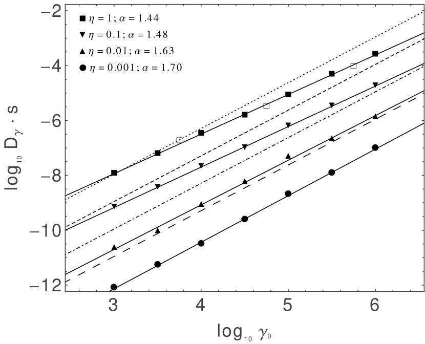
Figure 5: Energy diffusion coefficients as a function of particle Lorentz factor for Experiments 1–4 which sample various turbulence strengths, $\eta$. Solid shapes denote values for isotropic turbulence, and open squares denote values for anisotropic turbulence. The uniform magnetic field is $100\;\mu$G in every case. In addition, $n=100$ cm^-3, and $\lambda_{max}=0.1$ pc. Solid lines show fits to the isotropic turbulence data. Results obtained by quasi-linear theory as given by Eq. (17) are shown by the dotted ($\eta=1$), dashed ($\eta=0.1$), dot-dashed ($\eta=0.01$) and long-dashed ($\eta=0.001$) lines.

We plot the results of Experiments 1–4 in Figure 5 and Experiments 1, 4, and 5–8 in Figures 6 and 7 to illustrate how the diffusion coefficient index changes between the strong ($\eta\sim 1$) and weak ($\eta\ll 1$) turbulence limits. As predicted by quasi-linear theory, $\alpha\approx\Gamma$ when $\eta\ll 1$ for isotropic turbulence, with the best match occurring for Kolomogorov diffusion. However, Equation (17) overestimates the value of $D_{\gamma 0}$ by as much as two orders of magnitude. In addition, the indices decrease as the turbulence grows stronger, and quasi-linear theory does not appear to adequately describe the energy dependence for Kolmogorov ($\Gamma=5/3$) and Kraichnan ($\Gamma=3/2$) diffusion when $\eta\sim 1$.

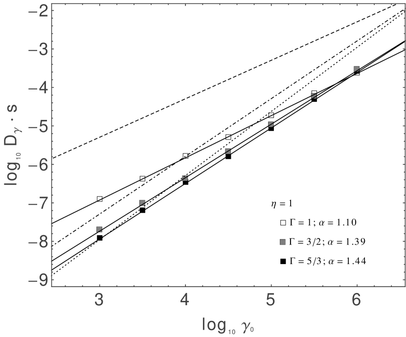
Figure 6: Energy diffusion coefficients as a function of particle Lorentz factor for Experiments 1, 5, and 7 (isotropic turbulence). The uniform magnetic field is $100\;\mu$G in every case. In addition, $n=100$ cm^-3, and $\lambda_{max}=0.1$ pc. Solid lines show fits to the data. Results obtained by quasi-linear theory as given by Eq. (17) are shown by the dotted ($\Gamma=5/3$), dot-dashed ($\Gamma=3/2$), and dashed ($\Gamma=1$) lines.

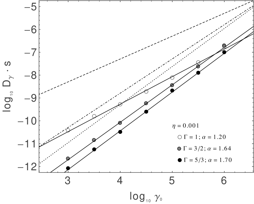
Figure 7: Energy diffusion coefficients as a function of particle Lorentz factor for Experiments 4, 6 and 8 (isotropic turbulence). The uniform magnetic field is $100\;\mu$G in every case. In addition, $n=100$ cm^-3, and $\lambda_{max}=0.1$ pc. Solid lines show fits to the data. Results obtained by quasi-linear theory as given by Eq. (17) are shown by the dotted ($\Gamma=5/3$), dot-dashed ($\Gamma=3/2$), and dashed ($\Gamma=1$) lines.

We next consider how the diffusion coefficients for Kolmogorov ($\Gamma=5/3$), Kraichnan ($\Gamma=3/2$) and Bohm ($\Gamma=1$) turbulence scale with $n$, $B_{0}$ and $\lambda_{max}$, but limit our analysis to the strong turbulence limit ($\eta=1$). Our results for Kolmogorov turbulence (derived from experiments 1 and 9–20) are shown in Figures 8–13. Specifically, Figure 8 illustrates the energy dependence of $D_{\gamma}$ for four values of ambient density $n$. As expected, a greater density yields a smaller Alfvén speed, and therefore a reduced energy diffusion. But the index $\alpha$ is not sensitive to $n$. We note that Equation (17) overestimates the energy diffusion coefficient for $\gamma_{0}\gtrsim 10^{3}$, and underestimates the energy diffusion coefficient for $\gamma_{0}\lesssim 10^{3}$. Figure 9 then illustrates the relation between $D_{\gamma}$ and $n$ for the value $\gamma_{0}=10^{5}$, where the fits from Figure 8 (along with fits to the data not shown if that figure) are used to obtain the plotted data points. The relationship between $D_{\gamma}$ and $n$ clearly takes on the same scaling obtained from quasi-linear theory, i.e., $D_{\gamma}\propto n^{-1}$. This result is expected since $D_{\gamma}\propto$ $(\Delta\gamma)^{2}\propto$ $(\delta E)^{2}\propto$ $v_{A}^{2}\propto n^{-1}$. We therefore assume that this scaling holds for all values of $\Gamma$.

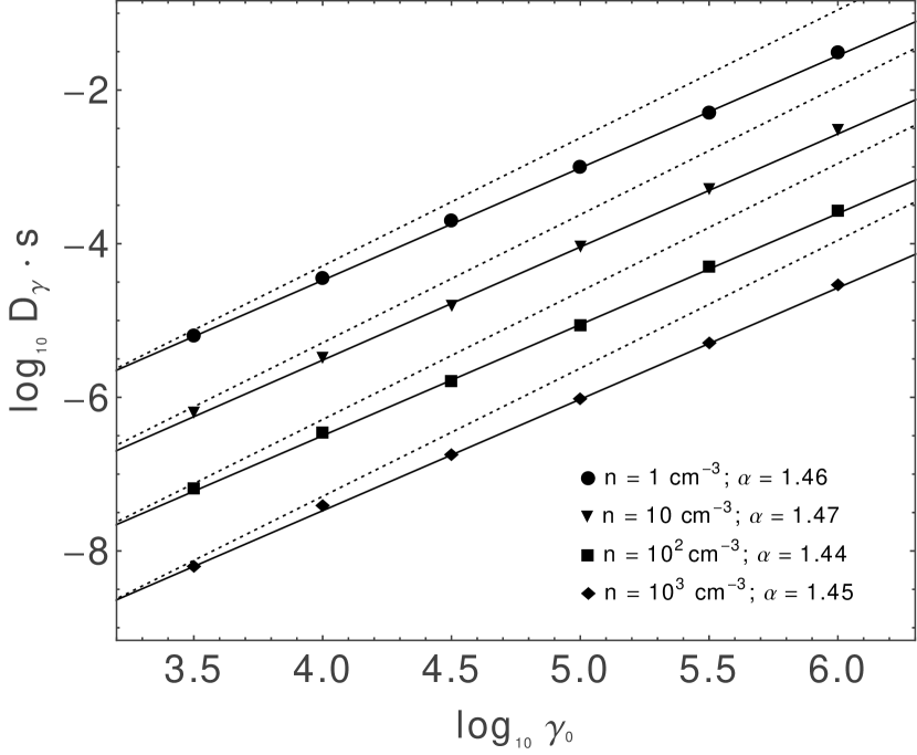
Figure 8: Energy diffusion coefficients as a function of particle Lorentz factor for Experiments 1,9, 11 and 14 (isotropic turbulence), which sample various ambient densities $n$. The uniform magnetic field is $100\;\mu$G, $\eta=1$, $\Gamma=5/3$, and $\lambda_{max}=0.1$ in every case. Solid lines show fits to the data, and dotted lines represent the results obtained by quasi-linear theory as given by Eq. (17).

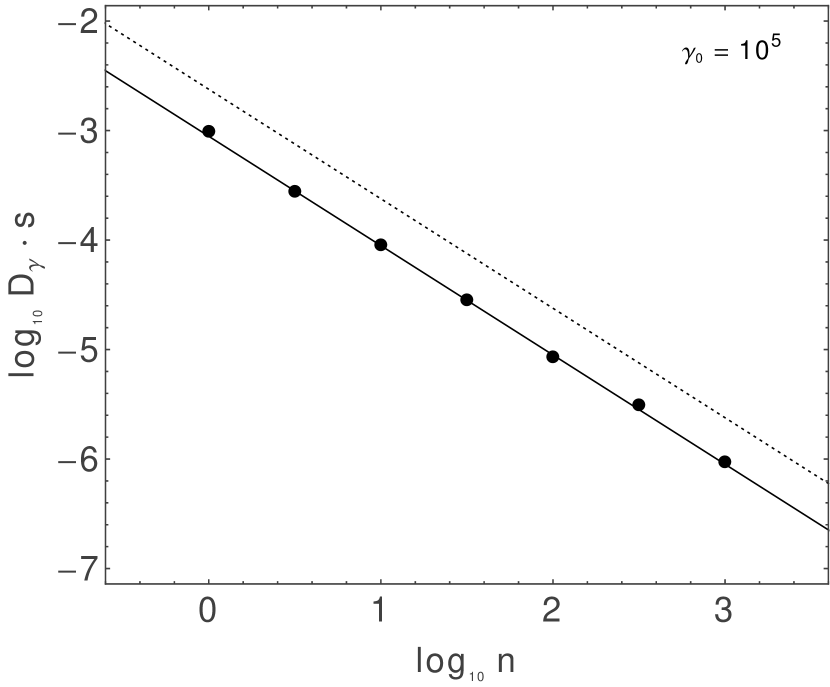
Figure 9: Energy diffusion coefficients for $\gamma_{0}=10^{5}$ as a function of density $n$ for Experiments 1 and 9 –14 (isotropic turbulence). The uniform magnetic field is $100\;\mu$G, $\eta=1$, $\Gamma=5/3$, and $\lambda_{max}=0.1$ in every case. The solid line show the fit to the data ($D_{\gamma}\propto n^{-1}$), and the dotted line represents the result obtained by quasi-linear theory as given by Eq. (17).

Figure 10 illustrates the energy dependence of $D_{\gamma}$ for five values of background field strengths $B_{0}$. Since a greater magnetic field strength leads to a greater electric field strength, energy diffusion increases with field strength. Again, the index $\alpha$ is not sensitive to $B_{0}$, but we find that Equation (17) overestimates the energy diffusion for larger values of $\gamma_{0}$, and underestimates the energy diffusion for smaller values of $\gamma_{0}$, although the transition varies depending on the field strength. Figure 11 illustrates the relation between $D_{\gamma}$ and $B_{0}$ for the value $\gamma_{0}=10^{5}$, where the fits from Figure 10 are used to obtain the plotted data points. We note that the scaling $D_{\gamma}\propto B_{0}^{2.50}$ obtained from our results differs from quasi-linear theory ($D_{\gamma}\propto B_{0}^{2.33}$).

Figure 12 illustrates the energy dependence of $D_{\gamma}$ for three values of $\lambda_{max}$. Again, the index $\alpha$ is not sensitive to $\lambda_{max}$, and once again, Equation (17) overestimates the energy diffusion for larger values of $\gamma_{0}$, and underestimates the energy diffusion for smaller values of $\gamma_{0}$. Figure 13 illustrates the relation between $D_{\gamma}$ and $\lambda_{max}$ for the value $\gamma_{0}=10^{5}$, where the fits from Figure 12 are used to obtain the plotted data points. As was the case with the field, the scaling obtained ($D_{\gamma}\propto\lambda_{max}^{-0.47}$) differs from that predicted by quasi-linear theory ($D_{\gamma}\propto\lambda_{max}^{-0.67}$).

Corresponding results for isotropic Kraichnan turbulence (derived from experiments 5 and 21–26) are shown in Figures 14–17, and for isotropic Bohm turbulence (derived from experiments 7 and 27–32) are shown in Figures 18–21. The analysis for these cases mirrors that described above for Kolmogorov turbulence, and the same general results are obtained.

Figure 10: Energy diffusion coefficients as a function of particle Lorentz factor for Experiments 1 and 15–18, which sample various background field strengths $B_{0}$. The particle density $n=100$ cm^-3, $\eta=1$, $\Gamma=5/3$, and $\lambda_{max}=0.1$ in every case. Solid shapes denote values for isotropic turbulence, and open shapes denote values for anisotropic turbulence. Solid lines show fits to the data, and dotted lines represent the results obtained by quasi-linear theory as given by Eq. (17).

Figure 11: Energy diffusion coefficients for $\gamma_{0}=10^{5}$ as a function of background field strength $B_{0}$ for Experiments 1 and 15–18 (isotropic turbulence). The particle density $n=100$ cm^-3, $\eta=1$, $\Gamma=5/3$, and $\lambda_{max}=0.1$ in every case. The solid line shows the fit to the data ($D_{\gamma}\propto B_{0}^{2.50}$), and the dotted line represents the result obtained by quasi-linear theory as given by Eq. (17).

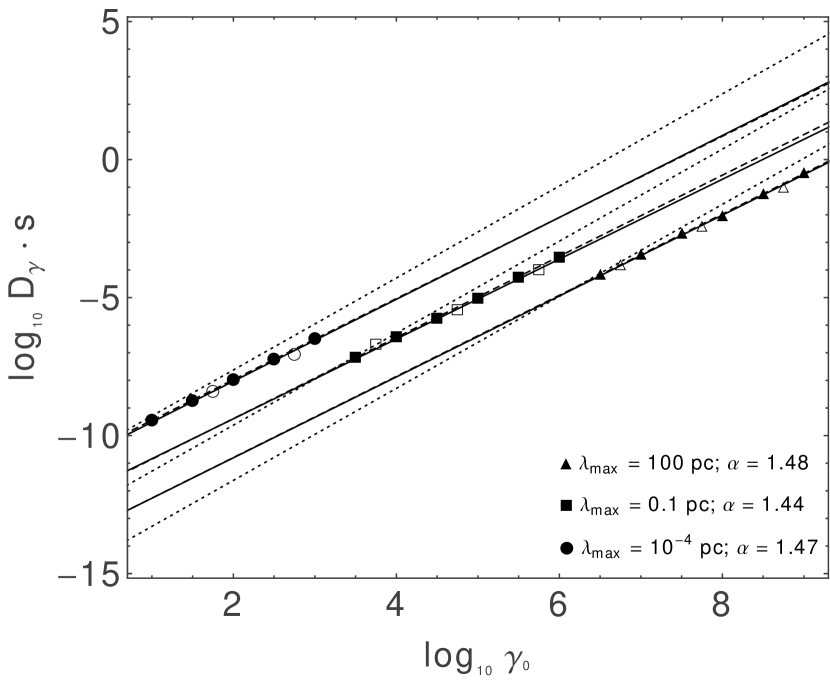
Figure 12: Energy diffusion coefficients as a function of particle Lorentz factor for Experiments 1 and 19–20, which sample various values of $\lambda_{max}$. The particle density $n=100$ cm^-3, background field strength $B_{0}=100\mu$G, $\eta=1$, and $\Gamma=5/3$ in every case. Solid shapes denote values for isotropic turbulence, and open shapes denote values for anisotropic turbulence. Solid lines show fits to the data, and dotted lines represent the results obtained by quasi-linear theory as given by Eq. (17).

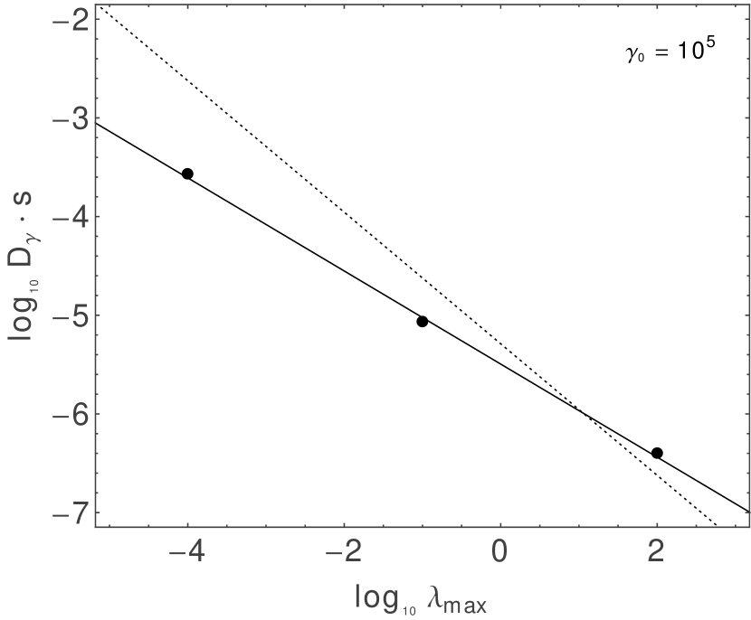
Figure 13: Energy diffusion coefficients for $\gamma_{0}=10^{5}$ as a function of $\lambda_{max}$ for Experiments 1 and 19–20 (isotropic turbulence). The particle density $n=100$ cm^-3, background field strength $B_{0}=100\mu$G, $\eta=1$, and $\Gamma=5/3$ in every case. The solid line shows the fit to the data ($D_{\gamma}\propto\lambda_{max}^{-0.47}$), and the dotted line represents the result obtained by quasi-linear theory as given by Eq. (17).

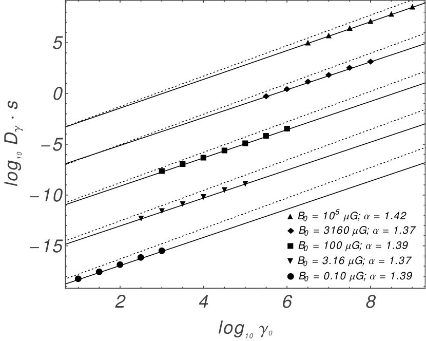
Figure 14: Same as Figure 10, but for $\Gamma=3/2$ and Experiments 5 and 21–24.

Figure 15: Same as Figure 11, but for $\Gamma=3/2$ and Experiments 5 and 21–24. The fit to the data (as shown by the solid line) yields $D_{\gamma}\propto B_{0}^{2.61}$.

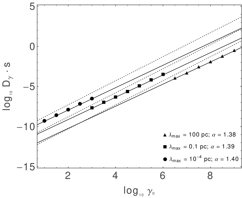
Figure 16: Same as Figure 12, but for $\Gamma=3/2$ and Experiments 5 and 25–26.

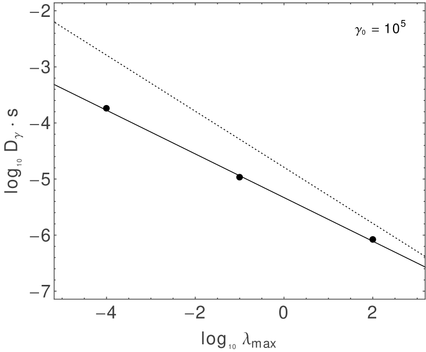
Figure 17: Same as Figure 13, but for $\Gamma=3/2$ and Experiments 5 and 25–26. The fit to the data (as shown by the solid line) yields $D_{\gamma}\propto\lambda_{max}^{-0.39}$.

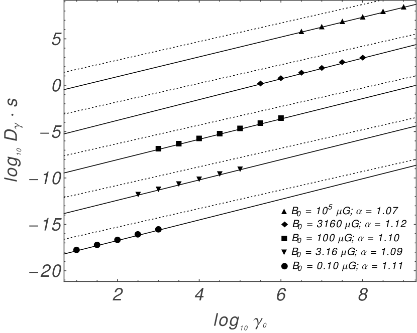
Figure 18: Same as Figure 10, but for $\Gamma=1$ and Experiments 7 and 27–30.

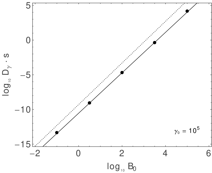
Figure 19: Same as Figure 11, but for $\Gamma=1$ and Experiments 7 and 27–30. The fit to the data (as shown by the solid line) yields $D_{\gamma}\propto B_{0}^{2.91}$.

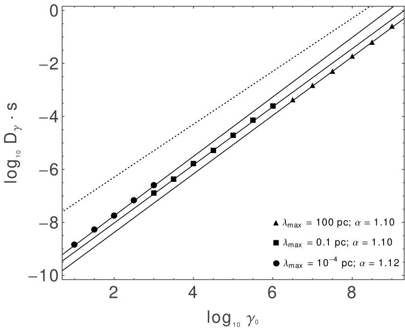
Figure 20: Same as Figure 12, but for $\Gamma=1$ and Experiments 7 and 31–32.

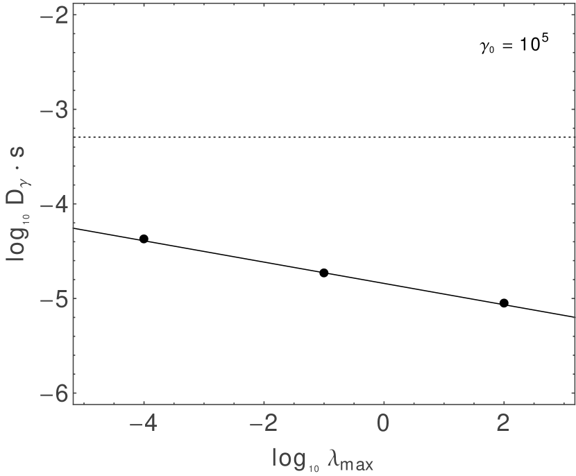
Figure 21: Same as Figure 13, but for $\Gamma=1$ and Experiments 7 and 31–32. The fit to the data (as shown by the solid line) yields $D_{\gamma}\propto\lambda_{max}^{-0.11}$.

Our results indicate that simple scaling laws of the form $D_{\gamma}=D_{\gamma 0}\,\gamma^{\alpha}$, where

$$D_{\gamma 0}=D_{0}\left({n\over 1\,{\rm cm}^{-3}}\right)^{-1}\left({B_{0}\over 1\,\mu{\rm G}}\right)^{\delta}\left({\lambda_{max}\over 1\,{\rm pc}}\right)^{\kappa},$$ (19)

can be used to obtain values of the energy diffusion coefficient over a wide range of parameters that pertain to turbulent interstellar and intergalactic environments, so long as the particle gyration radius $\lambda_{min}\ll R_{g}\ll\lambda_{max}$. In addition, the same expressions can be used to describe the isotropic and anisotropic cases in the limit of strong turbulence ($\eta\approx 1$).

We obtain values of $D_{0}$, $\alpha$, $\delta$ and $\kappa$ in the strong turbulent limit ($\eta=1$) for the three turbulence profiles considered in our work by using the results presented above. Specifically, final values of $D_{0}$ and $\alpha$, along with their $1\sigma$ errors, are obtained by finding the mean and standard deviations of the $D_{0}$ and $\alpha$ values from the corresponding experiments listed in Table 1. The values of $\delta$ and $\kappa$ are obtained from the fits to the data shown in figure 11 and figure 13 for $\Gamma=5/3$, figure 15 and figure 17 for $\Gamma=3/2$, and figure 19 and figure 21 for $\Gamma=1$. The results are summarized in Table 2.

Table 2: Fitting parameters

$\Gamma$		$D_{0}\,({\rm s}^{-1})$	$\alpha$	$\delta$	$\kappa$
5/3		$(1.6\pm 0.8)\times 10^{-16}$	$1.47\pm 0.02$	2.50	-0.47
3/2		$(3.7\pm 1.7)\times 10^{-16}$	$1.39\pm 0.02$	2.61	-0.39
1		$(7.6\pm 2.8)\times 10^{-15}$	$1.10\pm 0.02$	2.91	-0.11

We conclude our analysis by applying the results of this work toward obtaining estimates of the acceleration time $\tau_{acc}\equiv\gamma^{2}/D_{\gamma}$ required to energize protons up to energies of 1 TeV in molecular cloud environments. To keep this analysis as simple as possible, we assume that the magnetic field scales with density as given by Eq. (1). We also assume that the maximum turbulence wavelength $\lambda_{max}$ scales as the cloud size. Following Larson’s law (Larson 1981), we obtain the relation

$$\lambda_{max}=1600\,{\rm pc}\left({n_{H_{2}}\over 1\,{\rm cm}^{-3}}\right)^{-0.91}\,.$$ (20)

A plot of the acceleration time $\tau_{acc}$ as a function of molecular hydrogen density $n_{H_{2}}$ is shown in Figure 22 for Kolmogorov, Kraichnan, and Bohm turbulence. Given that clouds are not expected to last for more than $\sim 10$ Myrs, TeV cosmic ray production from stochastic acceleration of turbulent magnetic fields can clearly be ruled our for normal molecular cloud environments. We note, however, that the molecular clouds near the galactic center have fairly extreme environments. As shown in Fatuzzo & Melia (2012), the acceleration times is the GC environment are considerably shorter, as illustrated by the solid circle (inter cloud region at the GC) and solid square (molecular cloud at the GC) shown in Figure 22.

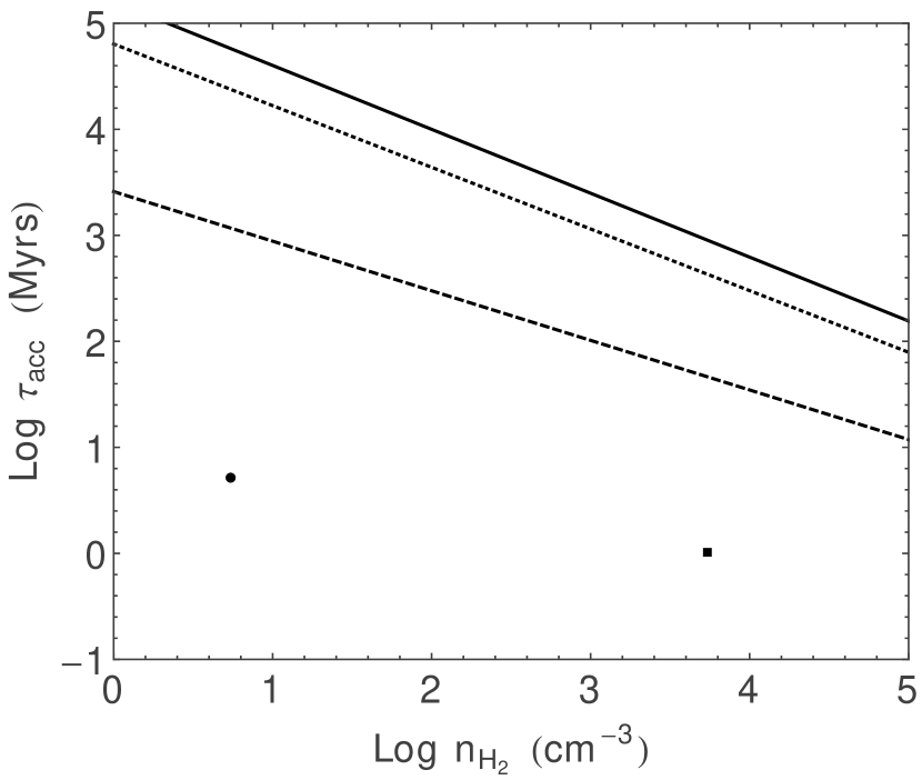
Figure 22: The acceleration time $\tau_{acc}\equiv\gamma^{2}/D_{\gamma}$ as a function of molecular hydrogen density for molecular cloud environments. The magnetic field is assumed to scale with density as per Eq. [1], and $\lambda_{max}$ is set equal to the size of the molecular cloud, where Larson’s Law is then used to relate $\lambda_{max}$ to the density $n_{H_{2}}$. The solid curve denotes the results obtained for $\Gamma=5/3$, the dotted curve denotes the results obtained for $\Gamma=3/2$, and the dashed curve denotes the results obtained for $\Gamma=1$. For comparison, the solid circle and solid square represent the acceleration times in the inter cloud region and molecular clouds at the GC, respectively (Fatuzzo & Melia 2012).

6 Conclusions

We have used a detailed numerical simulation to determine the spatial and spectral profiles of cosmic rays diffusing with arbitrary energy through turbulent media characterized by a broad range of magnetic fields, turbulence strength, fluctuation size and ambient particle density, for both isotropic and anisotropic turbulence. This study has expanded considerably from the initial attempt at simulating the behavior of relativistic particle propagation through the galactic-center environment, where they encounter a variety of physical conditions, inside and outside of the molecular gas in that region. Our goal throughout this exercise has been to avoid using “standard” techniques, e.g., quasi-linear theory or the diffusion equation, all of which are often subject to unknown factors that delimit the applicability of these approaches to real systems (but see also Nayakshin & Melia 1998; Wolfe & Melia 2006). Indeed, one of the prinicpal benefits of the technique we have developed in this work is an accurate determination of the spatial and energy diffusion coefficients that in turn may be used in these other approaches without the need to guess or estimate their normalization and energy dependence.

As the sensitivity and spectral range of high-energy observatories continue to improve, the need to accurately simulate the propagation of relativistic particles through turbulent media arises in an ever increasing range of environments, from the interstellar medium, to compact accretion regions surrounding supermassive black holes (such as Sgr A* at the galactic center), to the hot intracluster gas, and in even more exotic structures, such as the Fermi bubbles straddling the center of the Milky Way (Crocker & Aharonian 2011). However, the physical conditions characterizing these regions change considerably from one environment to the next. For example, the magnetic intensity may be as large as several Gauss near accreting black holes, but smaller than $0.01\;\mu$G in the intergalactic medium. We now know that quasi-linear theory is only approximately valid even in weakly turbulent environments, let alone regions where the turbulent magnetic energy is comparable to, or bigger than, the underlying uniform component. Worse, it is often difficult to estimate the absolute value of the diffusion coefficients without resorting to observational data which, however, are sometimes difficult to get (as in the case of the giant radio lobes in FR II galaxies).

These are among the reasons we have embarked on this type of investigation, to develop methods of handling the great diversity of physical conditions encountered by cosmic rays propagating through high-energy emitting environments. Previously (Fatuzzo & Melia 2010, 2012b), we reported some results of this study pertaining to the spatial diffusion coefficients. We found that the spatial diffusion of particles through turbulent fields is not sensitive to the minimum wavelength of the fluctuations, so long as the particle’s radius of gyration exceeds $\lambda_{min}$. For a given environment, as defined by $B_{0}$ and $v_{A}$, the diffusion process is thus dependent upon the maximum turbulence wavelength $\lambda_{max}$, the turbulent field strength, as characterized by $\eta$, and the turbulence spectrum, as characterized by the spectral index $\Gamma$.

We also noted that quasi-linear theory does not appear to be valid in the strong turbulence limit (see also O’Sullivan et al. 2009). We therefore investigated how the energy diffusion coefficient depends upon $\lambda_{max}$ and $\eta$ for Kolmogorov ($\Gamma=5/3$) turbulence, and found that the energy diffusion coefficients could be characterized as $D_{\gamma}\propto\lambda_{max}^{-0.47}$. This behavior is not consistent with quasi-linear theory, which instead predicts that $D_{\gamma}\propto\lambda_{max}^{-0.67}$ for Kolmogorov turbulence in the strong turbulence ($\eta\gtrsim 1$) limit. However, we also found that $D_{\gamma}\propto\eta^{1.2}$ in both the weak and strong turbulence limits.

But clearly, this initial sampling of the complex behavior of $D_{\gamma}$ under a variety of physical conditions is far from satisfactory. The purpose of the present paper has been to complete this work, finding scaling relations that one may use to calculate $D_{\gamma}$ under most conditions of interest, for all practical ranges of magnetic intensity, turbulence strength, ambient particle density, fluctuation size, and turbulence spectrum.

The empirical relations useful for this purpose have all been presented in §5. Broadly speaking, we have found that insofar as the energy diffusion coefficient $D_{\gamma}$ is concerned, quasi-linear theory predicts its correct energy dependence only for very weak, isotropic turbulence (i.e., $\eta\lesssim 0.01$). These predictions deviate substantially for $\eta\sim 1$, particularly for turbulence spectral indeces $\Gamma>1$, such as Kolmogorov turbulence, which seems to be prevalent in many diverse environments. For example, for the physical conditions one encounters at the galactic center (i.e., $B\sim 1-10^{3}\;\mu$G and $n\sim 1-10^{3}$ cm^-3), the actual index characterizing the dependence of $D_{\gamma}$ on $\gamma$ may be as small as $\sim 1.4$ instead of the predicted value $\sim 1.7$.

In addition, our results indicate that there is no difference in the energy diffusion of particles between isotropic turbulence and the anisotropic turbulence profiles predicted by Goldreich & Sridhar (1995) so long as the turbulence is strong ($\delta B\sim B$). On the other hand, our results indicate that anisotropic weak turbulence is considerably less effective in energetically scattering particles, consistent with the results of Chanrdran (2000).

Needless to say, if one is attempting to interpret the GeV Fermi spectrum of, say, the Fermi bubbles, in terms of an underlying population of cosmic rays, deviations from quasi-linear theory are rather critical, since the inferred particle distribution differs considerably from its injection point to where it emits the radiation, and the difference will be interpreted incorrectly with the inaccurate energy dependence predicted by these other techniques.

And not being sure of the normalization of $D_{\gamma}$ has its own challenges. For one thing, it is not possible to say anything definitive about the overall power being generated by the acceleration of these cosmic rays, which speaks directly to the mechanism associated with the relativistic particle injection, or even to the required density of dark-matter particles, if these cosmic rays are produced via dark-matter decays and collisions. But with our approach, it is not necessary to estimate the normalization of $D_{\gamma}$, because its absolute value is determined self-consistently from the statistical aggregate of numerous individual particle trajectories.

We have found that quasi-linear theory provides an acceptable estimate of the normalization of $D_{\gamma}$ at $\sim 1$ TeV energies, but can deviate considerably at lower energies, especially in the GeV range, and at energies exceeding $10-100$ TeV. A large factor responsible for these differences is the incorrect energy dependence predicted for $D_{\gamma}$. Obviously, if the normalization is adequate at $\sim 1$ TeV, the incorrect energy index will cause deviations at lower and higher energies.

Most importantly, however, our analysis has provided a method of determining not only the dependence of $D_{\gamma}$ on $\gamma$, but also its absolute value without the need to normalize it from the data. Having said this, one is not completely free of ambiguity, since one must still have an accurate estimate of the physical conditions, i.e., the magnetic field, the ambient density, and other characteristics that determine the state of the medium though which the cosmic rays are propagating. Fortunately, these conditions are easier to measure than the diffusion coefficients themselves, and in a more sophisticated use of our technique, in which MHD turbulence is simulated numerically rather than via the simple Kolmogorov or Bohm scaling relations, one can approach a level of realism not available to any of the other methods.

We look forward to the application of the scaling relations we have presented in this paper across a broad range of physical environments, allowing us to study high-energy sources with a level of accuracy commensurate with the detailed measurements now being made by the ever improving suite of space-based and ground-based observatories.

References

- (1) Adriani, O. et al. 2011, Science, Volume 332, 6025, 69
- (2) Aharonian, F. et al. 2006, Nature, 439, 695
- (3) Ballantyne, D., Melia, F., & Liu, S. 2007, ApJ Letters, 657, L13
- (4) Casse, F., Lemoine, M., & Pelletier, G. 2002, Phys. Rev. D, 65, 023002
- (5) Chandran, B. D. G. 2000, Phys. Rev. Lett, 85, 4656
- (6) Cho, J. & Vishniac, E. T. 2000, ApJ, 539, 273
- (7) Coker, R. F. & Melia, F. 1997, ApJ Lett, 488, L149
- (8) Crocker, R. M. & Aharonian, F. 2011, Phys. Rev. Lett.,106, 101102
- (9) Crutcher, R. M. 1999, ApJ, 520, 706
- (10) Falcke, H. & Melia, F. 1997, ApJ, 479, 740
- (11) Fatuzzo, M., Adams, F. C. & Melia, F. 2006, ApJ Letters, 653, L49
- (12) Fatuzzo, M., Melia, F., Wommer, E. & Adams, F. 2010, ApJ, 725, 515
- (13) Fatuzzo, M. & Melia, F. 2011, MNRAS, 410, L23
- (14) Fatuzzo, M. & Melia, F. 2012a, ApJ Letters, 757, L16
- (15) Fatuzzo, M. & Melia, F. 2012b, ApJ, 750, 21
- (16) Fraschetti, F. & Melia, F. 2008, MNRAS, 391, 1100
- (17) Giacalone, J. & Jokipii, J. R. 1994, ApJ Letters, 430, L137
- (18) Goldreich, P. & Sridhar, S., ApJ, 438, 763
- (19) Kowalenko, V. & Melia, F. 1999, MNRAS, 310, 1053
- (20) Kronberg, P. P. 1994, Reports on Progress in Physics, 57, 325
- (21) Lada, E. A., Bally, J., & Stark, A. A.1991, ApJ, 368, 432
- (22) Larson, B. L. 1981, MNRAS, 194, 809
- (23) Lis, D. C. & Goldsmith, P. F. 1989, ApJ, 337, 704
- (24) Lis, D. C. & Goldsmith, P. F. 1990, ApJ, 356, 195
- (25) Liu, S. & Melia, F. 2001, ApJ Letters, 561, L77
- (26) Liu, S., Melia, F., Petrosian, V. & Fatuzzo, M. 2006a, ApJ Letters, 647, L1099
- (27) Liu, S., Petrosian, V., Melia, F. & Fryer, C. L. 2006b, ApJ, 648, 1020
- (28) Lynn, J. W., Parrish, I. J., Quataert, E., & Chandran, B. D. G. 2012, ApJ, 758, 78
- (29) Lynn, J. W., Quataert, E., Chandran, B. D. G., & Parrish, I. J. 2013, ApJ, 777, 128
- (30) Markoff, S., Melia, F. & Sarcevic, I. 1997, ApJ Lett, 489, 47L
- (31) Markoff, S., Melia, F. & Sarcevic, I. 1999, ApJ, 522, 870
- (32) Melia, F. 2007, The Galactic Supermassive Black Hole, Princeton University Press (NY)
- (33) Melia, F. & Coker, R. F. 1999, ApJ, 511, 750
- (34) Misra, R. & Melia, F. 1993, ApJ Lett, 419, L25
- (35) Nayakshin, S. & Melia, F. 1998, ApJS, 114, 269
- (36) Ruffert, M. & Melia, F. 1994, A&A Lett, 288, L29
- (37) O’Sullivan, S., Reville, B., & Taylor, A. M. 2009, MNRAS, 400, 248
- (38) Paglione, D. T. A., Jackson, J. M., Bolatto, A. D., & Heyer, M. H. 1998, ApJ, 493, 680
- (39) Schlickeiser, R. 1989, ApJ, 336, 243
- (40) Wefel, J. 1988, in Genesis and propagation of cosmic rays; Proceedings of the NATO Advanced Study Institute (A88-37036 14-93), 1
- (41) Wolfe, B. & Melia, F. 2006, 638, 125
- (42) Wommer, E., Melia, F., & Fatuzzo, M. 2008, MNRAS, 387, 987
- (43) Yan, H. & Lazarian, A. 2002, Phys. Rev. Lett., 89, 281102