Impacts of planet migration models on planetary populations

Abstract

Context. Several recent studies have found that planet migration in adiabatic disks differs significantly from migration in isothermal disks. Depending on the thermodynamic conditions, that is, the effectiveness of radiative cooling, and on the radial surface density profile, planets migrate inward or outward. Clearly, this will influence the semimajor axis-to-mass distribution of planets predicted by population-synthesis simulations.

Aims. Our goal is to study the global effects of radiative cooling, viscous torque desaturation, gap opening and stellar irradiation on the tidal migration of a synthetic planet population.

Methods. We combined results from several analytical studies and 3D hydrodynamic simulations in a new semi-analytical migration model for the application in our planet population synthesis calculations.

Results. We find a good agreement of our model with torques obtained in 3D radiative hydrodynamic simulations. A typical disk has three convergence zones to which migrating planets move from the in- and outside. This strongly affects the migration behavior of low-mass planets. Interestingly, this leads to a slow type II like migration behavior for low-mass planets captured in these zones even without an ad hoc migration rate reduction factor or a yet-to-be-defined halting mechanism. This means that the new prescription of migration that includes nonisothermal effects makes the previously widely used artificial migration rate reduction factor obsolete.

Conclusions. Outward migration in parts of a disk helps some planets to survive long enough to become massive. The convergence zones lead to potentially observable accumulations of low-mass planets at certain semimajor axes. Our results indicate that more studies of the mass at which the corotation torque saturates are needed since its value has a main impact on the properties of planet populations.

1 Introduction

The huge diversity found in the properties of extrasolar planets is challenging to reproduce with global theoretical planet formation models. The goal of such a model is to explain all the different planet types, which range from low-mass rocky planets such as Kepler-10 b (Batalha et al., 2011) and multiplanet systems like our solar system to high-mass planets orbiting far from their star, such as NR 8977 (Marois et al., 2008).

The only way to study this problem is to use the results of global formation and evolution models and to compare them statistically with the steadily increasing number of known planets and their physical properties. This is done in planet populations synthesis calculations, in which the evolution of one or several planets and the harboring protoplanetary disk is calculated at the same time in Monte Carlo simulations to create whole populations of planets. Several groups presented studies based on this method, for example, Ida & Lin (2004),Ida & Lin (2010), Thommes et al. (2008),Miguel & Brunini (2008),Hellary & Nelson (2012), or by our group, Mordasini et al. (2009a),Mordasini et al. (2009b),Mordasini et al. (2012b),Mordasini et al. (2012a), and Alibert et al. (2011).

One general result found in all these models is that giant planets close to the star (“hot” Jupiters) do not form insitu: the extrapolation of disk properties found at larger distances to small distances indicates that there is probably not enough solid material close-in to form a sufficiently large core that whould be able to accrete gas. The amount of material a core can accrete locally is given by the isolation mass $M_{\rm iso}$. According to the empirical minimum-mass solar nebula model (MMSN), the isolation mass is only a fraction of the Earth mass ($\rm M_{\oplus}$) inside of 1 AU (Ida & Lin, 2004). Therefore an increase of solid matter by roughly two orders of magnitude compared with the MMSN would be needed (Ida & Lin, 2004). This means that to explain the close-in “hot” Jupiters, they would have to form initially at larger separations from the star and move inward by some mechanism (e.g., planet-planet scattering (Rasio & Ford, 1996), Kozai mechanism (Nagasawa et al., 2008), or tidal interactions with the gas disk (Goldreich & Tremaine, 1980; Tanaka et al., 2002)). In the planet formation model used in this work, we consider only one core per disk, which means that only migration caused by tidal interactions can be studied. This migration is generally described by two different regimes that depend on the mass of the protoplanet. The first is type I migration for low-mass planets, which are too small to form a gap in the disk, and the second is type II migration for planets that open a gap (D’Angelo et al., 2002).

In our previous work (e.g. , Mordasini et al., 2009a; Alibert et al., 2011), we used the results obtained for isothermal disks reported in Tanaka et al. (2002) to calculate type I migration rates. The migration rate in this model only depends on the disk surface density profile and not on the temperature profile of the disk because it assumes a globally isothermal disk. Migration rates obtained with this model always lead to rapid inward migration in disks with profiles similar to the MMSN. We showed (Mordasini et al., 2009a) that to obtain a synthetic population compatible with observations, one needs to artificially reduce the isothermal type I migration rate by a large factor. Ida & Lin (2004) used a similar type I migration prescription and found necessary reduction factors of $\lesssim 0.1$ for the migration rate.

Recent studies of type I migration in 2D or 3D hydrodynamical simulations also found outward migration for some masses or semimajor axes, depending on the disk temperature structure (Masset et al., 2006; Paardekooper & Mellema, 2008; Kley et al., 2009). More analytical work derived a formulation that could be used in planet population synthesis calculations (Casoli & Masset, 2009; Masset & Casoli, 2009, 2010). Finally, Paardekooper et al. (2010) derived a formalism for type I migration in adiabatic or locally isothermal disks and improved this even more in Paardekooper et al. (2011).

In the present work we describe a semi-analytical type I migration model that can be applied to a wider range of planet and disk properties than that of Paardekooper et al. (2011). For this we used the adiabatic and locally isothermal migration equations from Paardekooper et al. (2010) and ratios of relevant time scales to determine the transition between different regimes. We then studied the global consequences of the physics included in the migration model in new sets of population synthesis calculations.

As an overview of this work, the new semi-analytical model we created is introduced in Section 2, where we also compare torques obtained with this model with torques obtained with the model of Paardekooper et al. (2011) and data obtained in 3D radiative hydrodynamic simulations of Kley et al. (2009) and Bitsch & Kley (2011). We discuss in Section 3 a reference synthetic planet population calculated with the nominal model, and in Section 4 we study the effect of different migration models on planetary populations. In Section 5 we draw our conclusions and summarize our results.

2 Migration model

The migration module in our planet formation model (Alibert et al., 2004) distinguishes three main regimes, type I, disk-dominated type II, and planet-dominated type II migration (Armitage & Rice, 2005). Low-mass planets up to typically a few 10 Earth masses migrate in the type I regime, followed by migration in disk-dominated type II regime for more massive planets, which finally pass into planet-dominated type II migration when they reach masses of typically 100-200 $\rm M_{\oplus}$. We first describe our improvements to the description of the type II regime and introduce the new type I migration model afterwards.

2.1 Type II model and outward migration

In the old model, the type II migration rate was calculated using the equilibrium flux of gas in the disk, which was always assumed to be directed inward (Mordasini et al., 2009a). Now the direction and rate of type II migration is numerically calculated by considering the radial velocity $v_{\rm gas}$ of the (nonequilibrium) flux of gas at the position of the planet. It therefore allows outward migration if the planet is in a part of the disk where the gas is flowing outward (Veras & Armitage, 2004). The planetary migration rate is then

$$\dot{a}_{\rm p,T2}=v_{\rm gas}\times\rm{Min}(1,2\Sigma a_{\rm p}^{2}/M_{\rm p}),$$ (1)

where $a_{\rm p}$ is the semimajor axis of the planet, $M_{\rm p}$ is its mass, and $\Sigma$ is the gas surface density.

This mechanism has been invoked to explain the formation of exoplanets with semimajor axes larger than 20 AU, which cannot have formed in situ via the core accretion model (Veras & Armitage, 2004). However, we find in the syntheses using the nonequilibrium model that outward migration in type II is seldom important, and no large-scale net outward migration over more than $\sim 1\ AU$ typically occurs due to it. The reason is twofold:

The radius of velocity reversal (or of maximum viscous couple) $R_{\rm MVC}$ (Lynden-Bell & Pringle, 1974) is relatively close-in only early in the disk evolution. But, at these early times, the planets have usually not yet grown to a mass regime in which they migrate via type II. The evolution of the disk leads to the subsequent recession of $R_{\rm MVC}$ to larger radii. This occurs faster than the growth of the planets. Therefore type II outward migration is a very rare event during the spreading phase of the disk: at the moment planets have grown massive enough to migrate in type II, they are most of the time already located inside the $R_{\rm MVC}$.

Another chance of outward migration exists towards the end of the disk lifetime, when parts of the disk flow outward because mass is removed at the outer border due to external photoevaporation. The gas surface densities, however, are typically already quite low at the position of the planet at this moment, so that the reduction factor of the planet’s migration rate relative to the viscous velocity $\propto\Sigma a_{\rm planet}^{2}/M_{\rm planet}$ (see Alibert et al., 2005) is low as well, leading again to only modest amounts of outward migration. As in the original model, we assumed a linear reduction factor if $M_{\rm planet}>2\Sigma a_{\rm planet}^{2}$ (“fully suppressed” planet-dominated type II), because this agrees a better with hydrodynamical simulations than a square-root dependence on the planetary mass (Alexander & Armitage, 2009). Outward migration during effective photoevaporation is additionally limited because the remaining disk-lifetime is short.

2.2 Type I migration regimes

Here we discuss the migration of low-mass planets below a few tens of Earth masses. As mentioned above, one of the problems with the original description of orbital migration of low-mass planets is the short time scale found in isothermal type I migration (Tanaka et al., 2002), which resulted in too many close-in planets in planet population synthesis calculations (see also the comparison in Section 4.1.1). These rates had to be artificially reduced by correction factors to produce enough “cold” giant planets at larger semimajor axes (Mordasini et al., 2009b; Ida & Lin, 2008) to fit the observations.

On the other hand, Paardekooper & Mellema (2006) and Kley et al. (2009) showed that migration of small-mass bodies is not always inward because in a nonisothermal disk migration can be directed outward for some masses. Outward migration in the Type I regime can also occur in isothermal disks if full MHD turbulence is considered (see also Uribe et al., 2011; Guilet et al., 2013), but these new effects are not considered here because they need to be studied in more detail more studies before they can be parametrized.

Recently, Paardekooper et al. (2010) derived semi-analytical formulas for migration in the limiting case of adiabatic disks. Here we combine different formulas that are valid in different thermodynamical regimes into a model that can be applied to the wide range of planet masses and thermodynamic properties of the disk that are needed for our population-synthesis models.

2.2.1 Type I fit formula

Nonisothermal migration rates are more complex than isothermal rates. Generally, the gravitational interactions of the planet and the gas disk can lead to three characteristic flow regions that produce different types of torques:

• Lindblad torques:

  Gas sufficiently far from the planet is only slightly perturbed and orbits the star on nearly circular orbits inside or outside the planet’s orbit. The gravitational interaction generated by the planet in the regions outside and inside the corotation region produces the Lindblad torques.

• Corotation torque:

  If the orbit of a gas parcel is closer to the planet, its flow is more and more deflected, until it passes the planet’s orbit in front or behind the planet. Thus it forms so-called horseshoe orbits (see Fig. 1). The gas in the horseshoe orbits produces by deflection the so-called horseshoe drag or corotation torque. The strength of this torque depends on the thermodynamic regime of the interaction between the planet and the disk and the mass of the planet.

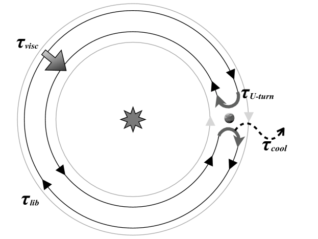
Figure 1: Schematic representation of the relevant time scales involved in type I migration. Flow lines of gas parcels are indicated in a system of reference that rotates with the planet. The planet is indicated on the right. In the center is the star. Close to the planet, the flow lines bend and make a u-turn during a time equal $\tau_{\rm u-turn}$. During that time, the gas on the flow lines cool on a time scale $\tau_{\rm cool}$. One full libration around the planet (indicated by the black lines) takes a libration time, $\tau_{\rm lib}$. During this time, viscosity acts on a viscous time scale $\tau_{\rm visc}$. The corotation region lies between the two black lines. Inside and outside this region, gas parcels do not make u-turns, but have a velocity relative to the planet because of to the Keplerian sheer (gray lines).

For typical properties (radially decreasing density and temperature) of the disk the Lindblad torques lead to inward migration, whereas the isolated torques from the corotation region can result in either inward or outward migration. For certain thermal and surface density profiles in the disk, these torques can be stronger than the Lindblad torques. Thus the combination of Lindblad and corotation torques can lead to either inward or outward migration, depending on their relative strength, which is determined by the disk properties.

The total torque $\Gamma$ can be expressed in the following way, as shown in Tanaka et al. (2002), Paardekooper et al. (2010) or Masset & Casoli (2010):

$$\tilde{\Gamma}=\frac{\Gamma}{M_{\rm p}} = \tilde{C}a_{\rm p}^{2}\Omega_{\rm p}^{2}\rm{\ \ \ ,where}$$ (2)

$$\tilde{C} = C\frac{a_{\rm p}^{2}}{h^{2}}\Sigma_{\rm p}\frac{M_{\rm p}}{M_{*}^{2}}=\frac{\dot{a}_{p}}{2a_{\rm p}\Omega_{\rm p}}=\frac{1}{4\pi N_{\rm orb}}=\frac{\tau_{\rm{orb}}}{4\pi\tau_{\rm{mig}}},$$ (3)

In these equation, $\tilde{\Gamma}$ is the specific torque (torque per unit mass). With a small p we denote all quantities of or at the position of the planet. $M_{\rm p}$ is the total mass of the planet and $a_{\rm p}$ the semimajor axis, while $M_{*}$ is the mass of the star, $h=H/a$ is the aspect ratio of the disk with a vertical scale height $H$. $\Omega_{\rm p}$ is the Keplerian frequency of the planet and $\Sigma_{\rm p}$ the gas surface density. The dimensionless factor $C$ in the second part of Eq. 3 gives the direction and strength of the migration and is discussed below for different thermodynamical regimes (Sect. 2.2). The dimensionless number $\tilde{C}$ is proportional to the migration rate $\dot{a}_{p}$ and inversely proportional to the number of orbits needed for a planet to migrate over the distance of its semimajor axis $N_{\rm orb}$. It is also proportional to the ratio of the two time scales for migration $\tau_{\rm{mig}}$ and orbital motion $\tau_{\rm{orb}}$

Additional parameters in the following equations are $\beta_{\rm\Sigma}$ as the local power-law exponent of the gas surface density ($\Sigma\propto r^{\beta_{\rm\Sigma}}$), $\beta_{\rm T}$ the local power-law exponent of the temperature ($T\propto r^{\beta_{\rm T}}$), and $\gamma$ the adiabatic index (ratio of the heat capacities) of the gas.

Depending on the properties of the disk, $C$ is a combination of various torque contributions of variable importance. Before we describe how we combined the contributions, we introduce expressions for their individual strength.

Paardekooper et al. (2010) derived that the Lindblad torque in an adiabatic disk is proportional to (their Eq. 47, part 1)

$$C_{\rm Lind}=\frac{1}{\gamma}\left(-2.5+1.7\beta_{\rm T}-0.1\beta_{\rm\Sigma}\right).$$ (4)

They also found that the horseshoe drag in the adiabatic case is proportional to (their Eq. 47, part 2)

$$C_{\rm HS,adia}=\frac{1}{\gamma}\left(1.65+\beta_{\rm\Sigma}(9-7.9/\gamma)-7.9\beta_{\rm T}/\gamma\right).$$ (5)

The coefficient $C$ in the adiabatic regime due to the combination of the Lindblad and corotation torques is

$$C_{\rm adia}=C_{\rm Lind}+C_{\rm HS,adia}.$$ (6)

Paardekooper et al. (2010) also found that the total torque in a locally isothermal regime, where the temperature $T$ is constant in time but not with semimajor axis, is proportional to (their Eq. 49)

$$C_{\rm loc}=-0.85+0.9\beta_{\rm T}+\beta_{\rm\Sigma}.$$ (7)

Subtracting from this the Lindblad torque in the adiabatic regime, but setting $\gamma=1$ (compare Paardekooper et al. (2010) Sect. 5.4 ), one finds the horseshoe drag part in the locally isothermal regime as

$$C_{\rm HS,loc}=1.65-0.8\beta_{\rm T}+1.1\beta_{\rm\Sigma}.$$ (8)

Compared with Eq. 4, Masset & Casoli (2010) derived a partially different Lindblad torque. We study the effect of this weaker Lindblad torque in Sect. 4.2.1.

$$C_{\rm Lind,2}=\frac{1}{\gamma}\left(-2.5+0.5\beta_{\rm T}-0.1\beta_{\rm\Sigma}\right).$$ (9)

2.3 Time Scales

The proper mix of the above described torque contributions can be determined by investigating the relevant time scales. For instance a disk behaving adiabatically produces a different torque than a locally isothermal one. Here the relevant time scales are the cooling time in comparison to the dynamic time.

To decide in which subtype the planet belongs to, we compared four characteristic time scales in total. The different time scales are schematically shown in Figure 1. In all the following estimates of the time scale, the important characteristic length scale is the width of the horseshoe region $x_{\rm s}$ given as (Masset et al., 2006; Baruteau & Masset, 2008; Paardekooper et al., 2010)

$$x_{\rm s}=1.16a_{\rm p}\sqrt{\frac{q}{h\sqrt{\gamma}}}.$$ (10)

In this equation $q$ is the ratio of the planet mass to the stellar mass.

The first two time scales we compared are the cooling time and the u-turn time to distinguish between the locally isothermal and the adiabatic regime. The u-turn time is the time a gas particle needs to undergo one turn in front or behind the planet. Its value is approximately given as (Baruteau & Masset, 2008)

$$\tau_{\rm u-turn}=\frac{64x_{\rm s}h^{2}}{9qa_{\rm p}\Omega_{\rm p}}.$$ (11)

The cooling time of a gas blob undergoing a turn is calculated by solving the 1D equation (Kley et al., 2009)

$$\frac{dT}{dt}=-\frac{1}{\rho C_{\rm V}}\frac{\partial}{\partial a}\left(F\right),$$ (12)

where $F$ is the heat flux, $\rho$ the gas density, and $C_{\rm V}$ the heat capacity at constant volume. We assumed a cooling over the length $l_{\rm cool}$, which is the minimum of $H$, and $x_{\rm s}$, which corresponds to either horizontal cooling over the width of the horseshoe region or vertical cooling through the disk. The flux $F$ in the optically thin case, when $\rho\kappa l_{\rm cool}<\sqrt{1/8}$ is $F=\tau\sigma T^{4}$, and in the optically thick case in the diffusion description $F=\frac{4acT^{3}}{3\rho\kappa}\frac{\partial T}{\partial a}$ (Kley et al., 2009). This means that we have two different types of the cooling time scale with a smooth transition when the optical depth is $1/\sqrt{8}$

$$\tau_{\rm cool}=\frac{l_{\rm cool}\rho C_{V}}{8\sigma T^{3}}\left(8\rho\kappa l_{\rm cool}+\frac{1}{\rho\kappa l_{\rm cool}}\right).$$ (13)

In a similar way we compared the viscous time scale and the libration time scale to find out whether the horseshoe drag is saturated or not (Masset & Casoli, 2010). The viscous time scale is

$$\tau_{\rm visc}=\frac{x_{\rm s}^{2}}{\nu},$$ (14)

while the libration time is given as (Baruteau & Masset, 2008)

$$\tau_{\rm lib}=\frac{8\pi a_{\rm p}}{3\Omega_{\rm p}x_{\rm s}}.$$ (15)

We denote the ratios of the relevant time scales as

$$s_{1}=f_{\rm cool}\frac{\tau_{\rm cool}}{\tau_{\rm u-turn}}$$ (16)

and

$$s_{2}=f_{\rm visc}\frac{\tau_{\rm visc}}{\tau_{\rm lib}}.$$ (17)

An equivalent approach can also be found in Casoli & Masset (2009) and Masset & Casoli (2009).

These time scales are typically order-of-magnitude estimates. Therefore, we introduced two factors, $f_{\rm cool}$ and $f_{\rm visc}$, of order unity to adjust the point of transition between different regimes to obtain a better agreement with radiative hydrodynamic simulations. In this work we set $f_{\rm cool}=1.0$, since this proved toagree well with numerical results of migration rates, as we show in Section 2.5. There, we also study the influence of various values of $f_{\rm visc}$. In general, we find that in nonirradiated $\alpha$ disks, planets transit from the locally isothermal into the adiabatic regime before the corotation torque saturates (Sect. 3.5).

We also note that for a given $h$, the ratio of the u-turn time and libration time is constant:

$$\tau_{\rm u-turn}=\frac{1.16^{2}8}{3\pi}\frac{h}{\sqrt{\gamma}}\tau_{\rm lib}\approx 1.14\frac{h}{\sqrt{\gamma}}\tau_{\rm lib}.$$ (18)

2.4 Type I migration formula

To combine the migration rates of these different regimes we defined an arbitrary transition function $z$ to obtain a smooth shift from the locally isothermal to the adiabatic regime as a function of the variable $s_{1}$:

$$z(s_{1})=\frac{1}{1+s_{1}^{b}},$$ (19)

which has the properties that for $s_{1}\rightarrow 0,z(s_{1})\rightarrow 1$ and for $s_{1}\rightarrow\infty,z(s_{1})\rightarrow 0$. Furthermore, depending on the value of $b$, the transition from 1 to 0 occurs more or less quickly around $s_{1}=1$. Therefore, uncertainties in overlap of different regimes can be approximated with a lower $b$ value. Additionally, the continuity of the transition function allows one to use longer numerical time steps in a simulation when the planet is close to the transition from one regime into another.

For individual transitions (e.g., locally isothermal to adiabatic, or type I into type II), other studies (Paardekooper et al. (2011); Masset & Casoli (2010)) derived physically motivated transition functions. But the comparison of physically motivated transition functions Paardekooper et al. (2011) with our simple transition function defined above shows little difference in population synthesis models (see Section 4.1.2). We set $b=4.0$, but the actual value of $b$ is again not very important for the global outcome seen in a population if $1.5\lesssim b\lesssim 100$ (see Appendix B).

We multiplied the horseshoe part with $\min(1/s_{2},1)$ to account for the saturation of the torque that originates in the horseshoe region. As shown in previous studies (Masset (2002) and Masset & Casoli (2010)), even when the cooling time is shorter than the u-turn time, and thus it is also much shorter than the libration time, viscosity is the driving factor for the saturation of the horseshoe region. This yields the following type I migration coefficient $C_{\rm T1}$ (in the second term of Equation 3):

$$C_{\rm T1}=C_{\rm Lind}+\min\left(1/s_{2},1\right)\left(z(s_{1})C_{\rm HS,loc}+\left(1-z(s_{1})\right)C_{\rm HS,adia}\right).$$ (20)

This assumes that even when cooling is much faster than the libration time scale the horseshoe drag will saturate without sufficient viscous coupling of the horseshoe region to the rest of the disk. The horseshoe part itself shifts between the adiabatic and the locally isothermal value depending on the ratio $s_{1}$ of the cooling time scale to the u-turn time scale (if $h$ is constant also with respect to the libration time scale (Eq. 18)).

The reduction of the surface density at the planet’s location due to the beginning gap formation for more massive planets will also modify the migration behavior. Crida & Morbidelli (2007) derived a formula to estimate the depth of the gap relative to the unperturbed disk. In their definition, a gap is formed when the surface density is reduced to 10% of the unperturbed value. They defined a factor (their Eq. 12)

$$P_{\rm\Sigma}=\frac{3h}{4\sqrt[3]{q/3}}+\frac{50\nu}{qa_{\rm p}^{2}\Omega_{\rm p}}$$ (21)

as a combination of two criteria (the thermal and the viscous condition) and used this factor to approximate the depth of the gap as

$$f_{\rm\Sigma}(P_{\rm\Sigma})=\begin{cases}\frac{P_{\rm\Sigma}-0.541}{4.0}&\text{if $P_{\rm\Sigma}<2.4646$ ,}\\ 1.0-\exp(\frac{P_{\rm\Sigma}^{3/4}}{-3.0})&\text{otherwise .}\end{cases}$$ (22)

We multiplied $\Sigma_{\rm p}$ in Eq. 3 with this factor to reduce the surface density in our torque calculations. This means that the type I migration rate is reduced by a factor of up to 10 at the point of transition to type II migration. This reduced type I migration rate is still about one order of magnitude higher than the type II migration rate for typical disk conditions (Sect. 2.5), which necessitates using a smooth transition function necessary.

Eventually, when the planet mass reaches the gap opening mass $M_{\rm gap}$, that is, the mass at which $f_{\rm\Sigma}=0.1$, the torque transitions to type II:

$$C=z\left(\frac{M_{\rm p}}{M_{\rm gap}}\right)C_{\rm T1}+\left(1-z\left(\frac{M_{\rm p}}{M_{\rm gap}}\right)\right)C_{\rm T2}.$$ (23)

We used the same functional dependency as in (Eq. 19) for a smooth transition from the type I to the type II torque. Here, we set the smoothing parameter $b=10.0$ (fast transition), because the reduction of the surface density already partly smoothes the transition (see Sect. B). The transition factor $s_{\rm typeII}$ is in this case the ratio of the planet mass to the mass at which the planet would open a gap in the disk:

$$s_{\rm typeII}=\frac{M_{\rm p}}{M_{\rm gap}}.$$ (24)

The factor $C_{\rm T2}$ is the corresponding type II migration coefficient in the same dimensions as $C_{\rm T1}$, given as

$$C_{\rm T2}=\frac{\dot{a}_{\rm p,T2}M_{*}h^{2}}{2a_{\rm p}^{3}\Sigma_{\rm p}q\Omega_{\rm p}}.$$ (25)

2.5 Comparison with other models

In this section we compare our model with that of Paardekooper et al. (2011) for a specific choice of parameters. The global consequences in a full planetary population are shown in Section 4.1.2. Here, we use a simple, nonevolving 1D-disk and compare the torques predicted by the two models in such a disk with results from the 3D radiation-hydrodynamic simulations of Kley et al. (2009) and Bitsch & Kley (2011).

Paardekooper et al. (2011) developed a more complex migration model trying to use first principles to derive in particular the transition functions compared with our model described in Sect. 2. They derived their torques by calculating the effect of viscosity and thermal diffusion onto the horseshoe region itself. From this they found transition functions between different parts of the corotation torque, using thermal diffusion time scales and viscous time scales as transition criteria between barotropic and entropy-related parts of the horseshoe drag and the linear corotation torque and also the saturation of both. On the other hand, we altered our torque according to the ratio of these time scales using an arbitrary transition. They called their ratio of these time scales $p_{\nu}$ and $p_{\chi}$ with $p_{\nu}^{2}$, the ratio scaling the saturation due to viscosity, being equal to our $s_{2}$ ratio if $f_{\rm visc}=0.75$. For $p_{\chi}$ one can show that

$$\frac{\pi}{3}p_{\chi}^{2}=\frac{1.16^{2}8}{9}\frac{h}{\sqrt{\gamma}}s_{1}.$$ (26)

The numerical factors in front of both sides of the equation are almost equal 1. The transition functions in Paardekooper et al. (2011) and our work are different. Therefore we considered the turnover points to compare the transitional behavior. In our model it occurs when $s_{1}=1$. For typical values of $h$ and $\gamma$ this leads to a value of $p_{\chi}\approx 0.2$. While not as easy to characterize due to the multiplication of several factors (see their Eqs. 23, 30, 31, and 53), this is in the range where the transition in the entropy torques occurs also in the model of Paardekooper et al. (2011). The main difference in the description is the separate treatment of the ”entropy” and ”barotropic” parts in Paardekooper et al. (2011) with three slightly different transition functions between different parts of the torque. We only used one transition function between the locally isothermal and adiabatic regime to attribute the dependence of the torque on cooling processes. Finally, they used only one free parameter, the smoothing factor for the planetary potential, which we set to 0.4 in our comparison here. They also stated that their model is mostly applicable to planets with a mass of a few Earth masses, while our model is intended to be applicable to a wider mass range.

To quantify the impact of the differences, we next compared the torques predicted by our simple model with those in 3D radiation hydrodynamic simulations, and also with the results found with the Paardekooper model. As will become clear, one finds that despite the simplifications in our model, we can fit the numerical results relatively well.

The 1D disk for the comparison was set up to be as similar as possible to the disk from the 3D simulations of Kley et al. (2009) and Bitsch & Kley (2011). The surface density $\Sigma$ is a power-law in semimajor axis with a fixed slope of -0.5, and the temperature $T$ is a power-law in semimajor axis of -1.5 inward of 2.5 $a_{\rm Jup}$, where $a_{\rm Jup}$ is the semimajor axis of Jupiter. Farther out, when the temperature almost reaches 10 K, its power-law exponent $\beta_{\rm T}$ increases and approaches 0. We used the same EOS (Saumon et al., 1995) and opacity tables (Bell & Lin, 1994) as in our full model. The viscosity was set to the same value as in Kley et al. (2009). All other disk parameters, such as disk height $H$ or density $\rho$, were calculated from $\Sigma$ and $T$. In this disk we then calculated the specific torques on planets of either different mass or different semimajor axes. With $\beta_{\rm\Sigma}=-0.5$ and $\beta_{\rm T}=-1.5$ there will be no type II torque since there is no radial gas flow in this disk. We stress that our disk model for the planet population synthesis calculations is in contrast a time-evolving 1+1D $\alpha$ model and is summarized in Sect. 3.1.

In Fig. 2 we plot torques from our model as a function of planetary mass and compare them with simulations from Kley et al. (2009), while in Figure 3, we compare our model with Bitsch & Kley (2011), where torques at different semimajor axes for a 20 $\rm M_{\oplus}$ planet were calculated. In both figures we also show the torque as predicted from the model of Paardekooper et al. (2011) (for their suggested optimal free parameter $b=0.4$).

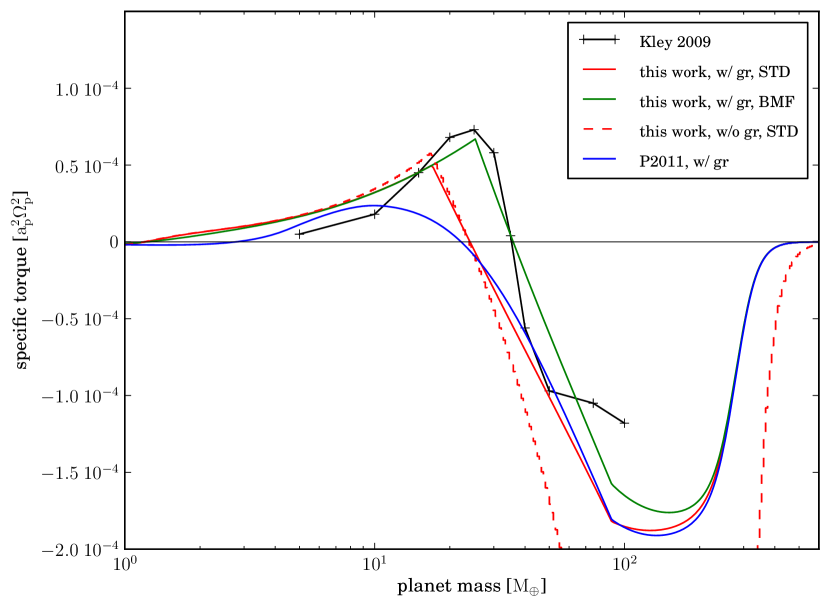
Figure 2: Specific torque for different planet masses in the range from 1 to 600 $\rm M_{\oplus}$ at 5.2 AU. The red solid line shows torques obtained with our nominal case ($f_{\rm visc}=1.0$), the green line is from the BMF model ($f_{\rm visc}=0.55$). The red dashed line does not include the reduction of the surface density due to gap formation (gr), otherwise it is identical to the nominal model. The black line with crosses shows torques from the 3D-radiative hydrodynamic simulations of Kley et al. (2009). A blue line shows torques obtained with the model of Paardekooper et al. (2011). The solid green line is our model of choice for the population synthesis models because it fits the results of full 3D simulations best.

We plot the migration rates for our model with and without the reduction of the surface density due to gap formation (solid and dashed lines respectively). This reduction was not only applied to our own model but also to the Paardekooper et al. (2011) prediction. For the dependency of planet masses (Fig. 2), the curves with the gap reduction remain closer to the data obtained by Kley et al. (2009). At around 200 $\rm M_{\oplus}$ when the transition to type II occurs, this factor causes a 10 times lower type I torque than without the reduction. Therefore with the zero type II torque in this disk-setup, the overall torque is also 10 times smaller. The red lines correspond to our model described above (with $f_{\rm visc}=1$: hereafter the STD ”standard”-model), while the green lines are our model with $f_{\rm visc}=0.55$ (hereafter the BMF ”best mass fit”-model). The latter value for $f_{\rm visc}$ was chosen to increase the saturation mass in a way so that the mass of zero torque in our own semi-analytical model agrees with the data of Kley et al. (2009). The associated reduction of transition parameter $s_{2}$ could be interpreted as a more efficient viscous injection of angular momentum into the horseshoe region from the rest of the disk than in the STD-model. Only a factor $\sim 2$ is needed to bring our model in agreement with the hydrodynamic simulations, meaning that the simple estimate of the transition using the characteristic time scales leads to relatively accurate results. Setting $f_{\rm visc}=0.55$ also increases the maximum specific torque, which follows the data from Kley et al. (2009) more closely than our model with $f_{\rm visc}=1$, or the model of Paardekooper et al. (2011), at masses larger than 15 $\rm M_{\oplus}$.

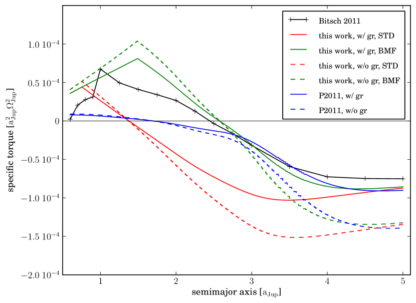
Figure 3: Specific torque for different semimajor axes in units of the semimajor axis of Jupiter $a_{\rm Jup}$ for a 20 Earth mass planet. The red lines show torques obtained with our STD model ($f_{\rm visc}=1.0$), the green lines with the BMF model ($f_{\rm visc}=0.55$). The solid (dashed) lines do (not) include the reduction of the surface density due to gap formation (gr). The line with black crosses shows torques found in the 3D-radiative hydrodynamic simulations of Bitsch & Kley (2011). The blue line shows torques obtained with the model of Paardekooper et al. (2011). The solid green line is our model of choice for the population synthesis models because it fits the results of full 3D simulations best.

In Figure 3 we compare torques on a planet of a fixed mass (20 $\rm M_{\oplus}$) as a function of semimajor axis. Here we see as well that the BMF-model provides the best agreement with the data of Bitsch & Kley (2011). The semimajor axis at which the torque vanishes is with 2.7 $a_{\rm Jup}$ relatively close to the 2.5 $a_{\rm Jup}$ found in the hydrodynamical simulations. The model of Paardekooper et al. (2011) places the position of zero torque at 1.8 $a_{\rm Jup}$, while in the STD-model it occurs at 1.4 $a_{\rm Jup}$. Thus, for planets closer than 2.5 $a_{\rm Jup}$ the BMF-model seems to be the best representation of both sets of numerical simulations.

At larger distance from the star the BMF-model and Paardekooper et al. (2011) again yield similar results and compare relatively well to the data. All curves also indicate that including the reduction of the surface density in Eq. 3 due to gap formation leads to a better agreement with the torques found in the hydrodynamic simulations, especially in the outer parts of the disk. In summary, we see that by setting $f_{\rm visc}=0.55$, the model agrees fairly well with the data provided from 3D simulations.

Some diskrepancy exists for the innermost point considered in the hydrodynamic simulation. It is most likely caused by effects of the change of the opacity due to ice evaporation, which is handled in a different way in our model vs. the 3D full models, so that the gradient of temperature and surface density differ.

Note that this comparison in principle only applies for a fixed value of the Prandtl number. The latter depends on $\gamma$ and the optical depth $\tau$ (Paardekooper et al. (2011)), which varies, for instance with the distance from the star or temperature. In the limit of high optical depth, the Prandtl number approaches $Pr=\frac{9}{4}\gamma(\gamma-1)$.

Nevertheless, we conclude that our BMF-model can quite adequately reproduce the current understanding of planet migration based on (semi-) analytical models for the modeling purpose of planetary populations.

2.6 Model versions

In the last section, we have calibrated our semi-analytical model with the results of a specific set of radiation-hydrodynamic simulations. With these results, we define three versions of the model that are used below to study the (global) effects of these different variants of our migration model:

• STD model In the standard version we simply set $f_{\rm visc}=1.0$ so that the plain time scales as defined in Section 2.3 are employed to calculate the point of saturation.

• BMF model In the best mass fit version we multiply $s_{2}$ by 0.55 ($f_{\rm visc}=0.55$). This model compares best with the 3D migration simulations as shown above.

• RED model In the reduced version we reduce $s_{2}$ by multiplying it with 0.125 ($f_{\rm visc}=0.125$). This results in a four times higher saturation mass than for the STD case. We use this even larger reduction to study the effect of different reduction factors.

3 Formation models and migration tracks

In addition to the comparison shown above for the migration rates alone, we are interested in the global effects of the new migration model onto a planet population compared with our older isothermal migration model. The planet formation model used for this is based on the paradigm of core accretion (Perri & Cameron, 1974; Mizuno et al., 1978; Pollack et al., 1996; Alibert et al., 2005). The model is described in detail in Alibert et al. (2005) with later modifications shown in Mordasini et al. (2009a), Mordasini et al. (2010, 2012a, 2012b), and Fouchet et al. (2012). It consists of different computational modules, namely the planet accretion module, the disk module, and the migration module. The migration module is described above and was used in recently published work of Fortier et al. (2013), Mordasini et al. (2012a), and Mordasini et al. (2012b). In the following sections we give a short overview of the disk and accretion modules. Then we present calculations of a few specific planets, show the associated formation tracks and the important features found in them. Finally, we present results from planet population synthesis calculations. Since we concentrate in this paper on the direct effects of the new migration model, we present here only simulations with just one embryo per protoplanetary disk. The interplay of migration and multiple concurrently forming planets (Alibert et al., 2013) will be addressed in future work.

3.1 Disk model

As a model for the protoplanetary disk, we used a 1+1D model as in Papaloizou & Terquem (1999) or Bell & Lin (1994), and present only a short summery here. The protoplanetary disk is described as a viscously evolving $\alpha$ disk, where $\alpha$ is assumed to be constant throughout the disk. The viscosity is given as $\nu=\alpha Hc_{\rm s}$ with $H$ the disk scale height and $c_{\rm s}$ the sound speed (Shakura & Sunyaev, 1973). Irradiation effects from the host star can be included in the calculations of the vertical structure (Fouchet et al., 2012). For the evolution of the gas surface density $\Sigma$ over time $t$ and distance $a$ from the star we solved the standard viscous evolution equation from Lynden-Bell & Pringle (1974). For most of our simulations in this paper we neglected stellar irradiation and used only viscous heating if not otherwise mentioned:

$$\frac{d\Sigma}{dt}=\frac{3}{a}\frac{\partial}{\partial a}\left[a^{1/2}\frac{\partial}{\partial a}\left(\nu\Sigma a^{1/2}\right)\right]+\dot{\Sigma}_{\rm w}(a).$$ (27)

As a sink term we included the photoevaporation rate $\dot{\Sigma}_{\rm w}(a)$ as given in Mordasini et al. (2009a). Together with $\alpha$ and the initial disk mass it determines the disk lifetime. At the start, the solid surface density of the planetesimals is equal to the gas density times the dust-to-gas ratio $f_{\rm D/G}$. It is further reduced inside of the iceline at a temperature $T=170\,\rm{K}$ by a factor of 4. Other than by accretion onto and ejection by the planet, we did not evolve the solid surface density.

3.2 Model of accretion and internal structure

We simulated the growth of one planet per disk. For this, we inserted a $0.6\,\rm M_{\oplus}$ seed embryo at a random position in the disk. The core has a constant density of $3.2\,\rm{g/cm^{2}}$ and contains all the heavy matter the planet accretes, that is, we assumed that all planetesimals sink to the core (Pollack et al., 1996). The seed will initially start to accrete mostly planetesimals, which leads to a growth of the core. The amount of energy released from the infalling planetesimals is high at this point and the core mass is low, therefore initially only small amounts of gas are bound. As the core grows, it binds an increasingly massive envelope. The accretion rate of gas is found by solving the standard equations of the structure of planet interiors, but with the simplification that the luminosity is constant throughout the envelope.

In the original model of Mordasini et al. (2009a), the luminosity of the planet is due to the accretion of planetesimals alone. This is usually the dominant source of luminosity at smaller masses (Pollack et al., 1996). Here, we adopted a simplified version of the model described in Mordasini et al. (2012b) to take also into account the luminosity generated by the accretion of gas. In the original model it was sufficient to consider only the luminosity due to the planetesimals, because the migration was always directed inward. This means that the cores always migrate into regions with a high solid surface density. With the new migration model, this is no longer the case: because the positive torques act at certain masses (see Section 2.5), it is possible that a core migrates through parts of the disk with a very low solid surface density content. There the luminosity of gas accretion becomes important.

3.3 Convergence zones

Figure 4: Strength of adiabatic migration coefficient $C_{\rm adia}$, plotted as a function of semimajor axis at times equal 0.02 , 0.1 and 0.5 Myr in a nonirradiated, evolving $\alpha$-disk. Positive values of $C_{\rm adia}$ drive outward migration.

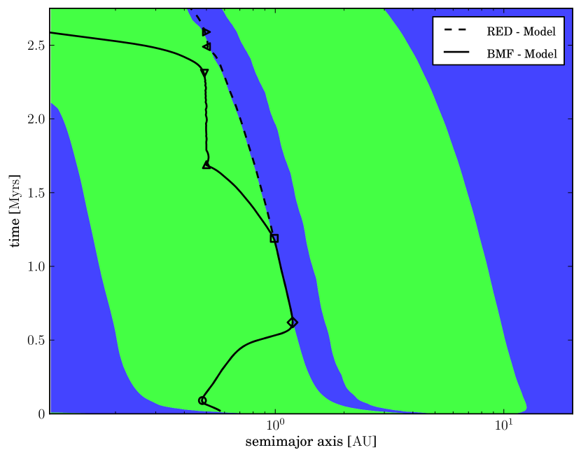
Figure 5: Direction of migration in the adiabatic migration regime for a nonirradiated evolving $\alpha$-disk. Blue indicates regions of inward migration while green shows outward migration. The black lines are the migration tracks of an evolving protoplanet set into the disk at  2000 yr. The track shown with the solid line uses the BMF migration model while the dashed line is calculated with the RED model (see Sect. 3.4). The symbols mark important points in the evolution and are discussed in the text.

These positive torques lead to regions in a disk where a planet within the adiabatic migration regime migrates outward instead of inward (Lyra et al., 2010; Mordasini et al., 2011). Figure 4 shows the values of $C_{\rm adia}$ (which represents the strength of the migration in the adiabatic regime, see Eq. 6) at time equal 0.02, 0.1 and 0.5 Myr in a nonirradiated evolving $\alpha$-disk with $\Sigma_{0}=420\ \rm{g/cm^{2}}$ and $\dot{M}_{\rm w}=6.7\times 10^{-9}\ \rm M_{\odot}/{\rm yr}$. These parameters results in a lifetime of the disk of 2.8 Myr.

In Figure 4 one can see two regions of outward migration, i.e., with positive values of $C_{\rm adia}$, from 0.46 AU to 2.6 AU and farther out from 3.6 AU to 11.5 AU at 0.02 Myr (red curve). At later times these regions are closer to the star as the disk evolves. To further illustrate the time evolution of the regions in Figure 5 we show the direction of migration as a function of time for this disk. Blue indicates regions of inward migration while green shows outward migration. One can see that these regions slowly move inward as the disk evolves. This occurs on the viscous time scale of the disk (Lyra et al., 2010). Owing to the existence of the outward and inward regimes, there are special locations in the disk. For example, at an age of 0.5 Myr, the migration changes from outward to inward at 10 AU (and at about 1.2 AU) when moving to a larger distance (i.e., these are points of zero torque where the derivative of the torque with distance is additionally negative). Such a point is called a convergence zone (CZ). It is called this because planets in its vicinity converge on this zone from both inside and outside (see Lyra et al., 2010). The domain in orbital distances from which planets migrate to the convergence zone is the associated convergence region. At 0.5 Myr, the inner convergence region extends from 0.2 to 1.8 AU for example. Similar results for two convergence zones for various disk models were also recently presented by Kretke & Lin (2012) and Yamada & Inaba (2012). After reaching the convergence zone, a planet remains slightly outward, but close to it, so that the net torque pushes the planet inward at the same migration rate as the zone itself.

Once captured in a convergence zone, the planet migrates on a time scale that is at least an order of magnitude longer than typical type I migration time scales. For example, while captured in the inner convergence zone, the planet discussed below has an equivalent migration coefficient $C$ (Eq. 3) of 0.034 while $C$ is during normal type I migration on the order of 1 as shown for instance in Fig. 4 or Paardekooper et al. (2010).

However, for some conditions, a low-mass planet cannot migrate at a sufficiently high rate to remain close to the CZ. Instead, the planet leaves the CZ and falls behind it (the planet still migrates inward, but is overtaken by the CZ). This occurs especially for the inner convergence zone. Typically, after leaving the inner zone, the planet transitions into the outer one, where it is again captured. The reason is that the type I migration rate is proportional to the planet mass. For a sufficiently low mass of the planet, the type I migration time scale thus becomes longer than the viscous time scale of the disk, which sets the speed at which the CZ moves. This characteristically occurs at the end of the disk lifetime, when the gas surface density is low, so that the type I migration time scale becomes even longer.

The position of the inner CZ is close to the distance of the local minimum in the opacity at a temperature of $\approx 200K$ (Lyra et al., 2010), which is the temperature where ice grains are completely molten in the opacity law of Bell & Lin (1994). The change in the slope of the opacity at this point leads to a change in the temperature power-law exponent $\beta_{\rm T}$, which leads to the change of the sign of $C_{\rm adia}$ and therefore to a convergence zone. The reason for the outer CZ is the change of the temperature slope due to the convergence onto the background temperature in the outer part of the disk.

The convergence zones only exist for a certain range of planet masses (Kretke & Lin, 2012). A low-mass planet will migrate in the locally isothermal regime since the thermal processes in the disk are fast enough to regulate the temperature during a u-turn of the gas. On the other hand, when a planets becomes massive enough, the angular momentum flux through the horseshoe region will be too low to support the unsaturated horseshoe drag, so this part of the torque saturates and in general rapid inward migration sets in.

3.4 Migration and formation tracks

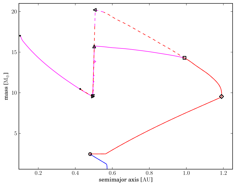
Figure 6: Formation tracks, i.e., evolution of the position in the distance-mass plane for a planet in a nonirradiated, evolving $\alpha$-disk. The track shown as a solid line uses the BMF migration model, while the dashed line uses the RED model. The colors represent the different migration regimes and are also used in this way in subsequent figures. Blue shows unsaturated locally isothermal migration, while red shows unsaturated adiabatic and magenta saturated adiabatic migration. In both cases the planet does not enter the type II or the saturated locally isothermal regime. The symbols mark the same important points in the evolution as in Fig. 5 and are discussed in the text. The small filled circles show the final positions of the planets at the end of the simulations.

The new migration model leads to changes in the evolution of a protoplanet that are different from those described in Mordasini et al. (2009a). We discuss the new behavior in this section where we show the migration and formation tracks of a typical protoplanet of our synthesis simulation. Not every evolving protoplanet in our calculations shows every behavior described below, but most evolutionary tracks of planets feature at least some part of the behavior. The consequences of the new migration model for a whole synthetic population are studied after this.

Further to what was discussed before, Figure 5 also shows two tracks of an evolving protoplanet starting at 0.57 AU at  2000 yr after the start of disk evolution. Figure 6 shows the corresponding formation tracks of this protoplanet in the semimajor axis mass plane. In both diagrams, the simulation represented by the solid line uses the BMF migration model, where $f_{\rm visc}=0.55$, while the dashed line is used for the RED model with $f_{\rm visc}=0.125$ (see Sect. 2.6), simulating a larger saturation mass. The beginning of the evolution of the protoplanet is the same in both models. It starts to migrate inward in the locally isothermal migration regime (blue part of the track in Figure 6) and accretes solids from its surrounding, depleting this part of the disk of planetesimals. When it reaches a mass of approximately 2.5 $\rm M_{\oplus}$, its horseshoe region is broad enough that cooling cannot keep the gas that is on horseshoe orbits in a locally isothermal state. The planet enters the unsaturated adiabatic regime, shown in red in Figure 6, and starts to migrate outward (at the position marked by a circle in the figures). This occurs at 0.1 Myr as seen in the migration track in Figure 5. While migrating outward, the planet does not grow at first because there is almost no solid material left because of its previous passage through this part of the disk. The protoplanet is also still too small to accrete significant amounts of gas. After crossing its initial position, growth by accretion of planetesimals sets back in and the planet migrates outward until it enters the convergence zone at 0.6 Myr (diamond symbol). Here the direction of migration again changes to inward as the planet is now bound to the CZ. While the disk evolves, this zone and the captured planet move slowly inward. The planet again moves through a region that is depleted of almost all planetesimals. But, with a 10 $\rm M_{\oplus}$ core, the planet is now massive enough to bind nebular gas in its envelope. This is especially true when there is not much solid accretion, which means that the core luminosity is low, and therefore the gas accretion rate is high. The planet grows by accreting gas, until at about 1.25 Myr in the BMF model (solid line), it reaches the mass where saturation sets in (square symbol). The positive horseshoe drag is reduced with increasing mass and is not sufficient to counterbalance the negative Lindblad torques. The planets therefore leaves the CZ and rapidly migrates inward (saturated adiabatic migration regime, magenta in Fig. 6).

The planet continues to accrete gas until the inner edge of its feeding zone reaches the distance of the previous closest approach to the star (upward-facing triangular symbol). Again in reach of planetesimals, solid accretion restarts and increases the core luminosity. The envelope expands, heated by this process, and because it is still connected to the disk at this time (attached phase, see Mordasini et al., 2012b), the heating leads to the loss of envelope mass and a corresponding reduction of the total planetary mass (see Sect. 3.2). This reduces the level of saturation, which in return increases the horseshoe drag, which can again balance the Lindblad torque resulting in an almost complete stop of migration: if the planet were to migrate outward again, solid accretion would stop and rapid gas accretion would start to increase the mass. This would reduce the horseshoe drag and push the planet back inward. In the opposite case of further inward migration, solid accretion would become stronger. This would increase the core luminosity and remove more envelope mass, and the total mass decreases. This would increase the outward-directed horseshoe drag because of the reduced saturation of the corotation torques. The planet would thus tend to migrate outward. The combination of these two points means that the planet has reached a quasi-stable point due to the interplay of accretion and migration.

With the evolution of the disk, the saturation mass at a given point in the disk decreases over time. Thus the mass where the partly saturated horseshoe drag balances the Lindblad torques is also reduced with time. Because of the interaction of accretion and migration, the planet’s mass remains exactly at this zero-torque mass.

The planet is forced to loose more mass and therefore remains at this semimajor axis for a given moment in time, while, as a result, the planet moves in slowly over longer time scales. It just “nibbles” on the edge of the planetesimal disk that was depleted up to this distance, while reducing its mass. The gas envelope mass is decreased until a level is reached that the planet can support with the full solid accretion rate of normal inward migration.

In case of the BMF model, this is a slow process. The protoplanet remains for 0.5 Myr at 0.5 AU while it looses 6 $\rm M_{\oplus}$ of the envelope it has accreted while moving inward in the CZ and later in the saturated adiabatic migration regime. At this time it has only 0.1 $\rm M_{\oplus}$ of envelope left. This is the same amount as at the time it became bound to the CZ. The RED model and its increase of the saturation mass leads to a slightly different behavior of the protoplanet. It remains for a longer time in the CZ and can thus accrete gas for a longer time than the BMF model protoplanet. This results in a larger envelope mass when it reaches the distance of the previous closest approach (left-facing triangle). But since in both cases the protoplanet migrated through the same part of the disk, both have the same amount of solids accreted and thus the same core-mass. Therefore, the increase of the solid accretion rate also leads to a mass loss of the envelope in the RED model case. But here, the planet is still in the unsaturated migration regime while loosing most of its envelope mass. Therefore, the mass loss does not lead to a change in the migration rate. The protoplanet is still bound to the CZ and is pushed by it into the remaining planetesimal disk. Therefore, the mass loss occurs much faster here, the planets looses  11 $\rm M_{\oplus}$ in only  0.1 Myr.

This illustrates the strong inter-dependence of migration and accretion. The solid accretion rate is set by the amount of solids reachable by the planet, and therefore by the migration that brings the protoplanet into new regions of the disk. But this behavior is only true if the availability of planetesimals themselves, and not the collision rate, is the limiting factor for the solid accretion rate $\dot{M}_{\rm core}$. In the planet-envelope structure model used here, the solid accretion rate, the associated core luminosity, and the mass of the core itself define the envelope structure and thus the envelope mass of a planet.

The small loops in the track that occur while the planet in the BMF model looses mass (between the up- and down- facing triangles) are caused by a finite time-step. Some larger loops are visible in the formation tracks in Figure 7. We show here the data obtained during the population synthesis calculations discussed in Sect. 3.5 and shown in that figure. We also separately simulated the same case with a much shorter time-step and obtained the same results without these small loops.

We did not consider an increase in the random velocities of the planetesimals due to the presence of a planet. They remain small, as reported in Pollack et al. (1996). A more realistic oligarchic growth model as described in Fortier et al. (2007) and Fortier et al. (2013) leads to higher random velocities and thus a smaller focusing factor in the calculation of the solid accretion rate $\dot{M}_{\rm core}$. This would lead to less envelope loss if $\dot{M}_{\rm core}$ remains small enough.

Another point to consider, in addition to the planetesimal accretion rate, is the treatment of the protoplanetary disk in our model. We did not let the disk evolve except for depletion due to accretion onto the protoplanet. Therefore there is a sharp edge into which the planet can migrate. A more realistic treatment (e.g., planetesimal drifting or diffusion, scattering) would lead to a gradual increase of $\dot{M}_{\rm core}$ and thus to a slower loss of the envelope. But we expect the final outcome to be similar, only the track in the a-M plane would be smoother (mass loss setting in earlier and more gradually).

In both cases shown here, the protoplanet starts again to accrete solids and nebula gas and migrates inward after it looses almost all its envelope mass (down- respectively right-facing triangles in Fig. 5 and 6). In case of the BMF model it migrates in the faster saturated adiabatic migration regime until in reaches 0.1 AU and a final mass of  17 $\rm M_{\oplus}$ ( 0.9 $\rm M_{\oplus}$ in its envelope) and the simulation stops. In the RED model the simulation ends with the disappearance of the disk at 2.8 Myr and the planet migrated to 0.43 AU with a mass of  10.5 $\rm M_{\oplus}$ (only 0.1 $\rm M_{\oplus}$ in the envelope).

3.5 Reference population synthesis calculation

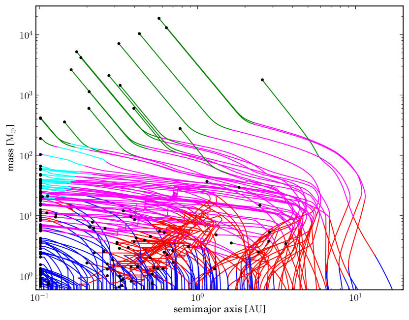
Figure 7: Formation tracks, the evolution of the position of the planets in the semimajor axis mass diagram. Color shows the different migration regimes at this point of its formation. Blue shows unsaturated locally isothermal, cyan saturated locally isothermal migration, red shows unsaturated adiabatic and magenta saturated adiabatic migration, finally, green shows type II migration. The filled circles show the final positions of the planets at the end of the simulations.

Quantity	value
Initial disk power-law exponent	-1.5
Disk viscosity parameter $\alpha$	$7\times 10^{-3}$
Inner radius of computational disk	0.1 AU
Outer radius of computational disk	50 AU
Gas surface density at inner radius	continues
Irradiation for disk temperature profile	not included
Iceline	included
Embryo starting mass	0.6 $\rm M_{\oplus}$
Core density	$3.2\rm{g/cm^{2}}$
Envelope type	primordial H2/He
$dl/dr$ in the envelope	zero
Grain opacity reduction factor	1.0
Type I migration	BMF-model
Type I migration reduction factor	none
Transition criterion type I to type II	Crida et al. (2007)
Transition exponent
Type I to type II migration (Eq. 23)	10.0
Transition exponent
Unsat. to saturated migration (Eq. 20)	4.0
Cooling reduction factor $f_{\rm cool}$	1.0
Viscosity reduction factor $f_{\rm visc}$	0.55
Stellar mass	1 $\rm M_{\odot}$
Simulation duration	till gas disk vanishes
Number of embryos per disk	1

Table 1: Parameters and settings for the reference population synthesis.

After studying the single case, we now look at a population synthesis calculation with 10000 different initial conditions that we used as our reference when we investigated the effects of different migration models on a synthetic planet population. The important parameters of the synthesis can be found in Table 1. We used the BMF-migration model and an $\alpha$ parameter of $7\times 10^{-3}$ for the nonirradiated disk.

Figure 7 shows the tracks of 250 cases, the different migration regimes color coded. The meaning of the colors is described in the caption of Fig. 7. One can see that most planets start in the locally isothermal migration regime, changing into the unsaturated adiabatic migration regime before the horseshoe drag saturates and they migrate inward. Some are large enough to transition into type II migration while others end up at 0.1 AU. Two groups corresponding to the inner (inside of 1AU) and outer (outside of 1 AU) convergence zone are visible in Fig. 7.

Figure 8: Final position of the synthetic planets in the semimajor axis mass diagram. Color shows the different migration regimes a planet is in when the calculation ended. The meaning of the colors is the same as in Fig. 7. The bars at 0.1 AU indicate the mass range of the “hot” planets in the different regimes. The boxes indicate clusters of planets described in the text.

When a planet migrates outward through the iceline, the migration rate does not change, but its solid accretion rate does change by a factor of 4, because the increase in the solid surface density. This results in a bend and a much steeper slope in some of the tracks in the outer zone. Horizontal parts in the formation tracks that indicate migration without growth are also lacking in the tracks of the outer planets. In the outer parts, especially outside of the iceline, the amount of solid matter is too large to be completely accreted onto the planet at the given accretion rates $\dot{M}_{\rm core}$. Thus, planets can also collect material on their second pass through a part of a disk and grow.

The inner and outer CZ are the reason for three groups of planets in the final position a-M diagram. They can be seen in Figure 8. A fourth possible cluster is not visible because the BMF-migration model leads to a situation where all those planets migrate inward of 0.1 AU (see Section 4.2.2):

• The first cluster, which is the one with the highest number of planets, lies approximately between 0.15 and 0.8 AU and  1 and  20 $\rm M_{\oplus}$ (red box in Figure 8). It consists of planets captured by the inner convergence zone. Most of the planets are directly attached to the CZ when the disk disappears and the simulation stops. Their mass is too small for a transition into saturated migration and departure of the CZ. A strip of planets extends inward from this cluster. These planets saturated shortly before the disk ended. However, most planets that transition into the saturated migration regime while being in the inner CZ eventually end up at 0.1 AU.

• The second cluster lies farther away from the star (1 AU to 4 AU) but is also in the mass range between  1 and  20 $\rm M_{\oplus}$ (blue box in Figure 8). It consists of planets captured by the outer second CZ. It is less populated because fewer embryos start at the larger distances because the distribution of the starting positions, which are uniform in log($a$). Additionally, the amount of solid material to grow is larger, thus many planets at these distances can reach masses above the saturation mass.

• The third cluster consists of planets that saturated while being in the outer convergence region (green box in Figure 8). But they are massive enough and can accrete enough solids on their way in that most of them can transition into type II migration. Here they migrate on the time scale of the disk evolution or slower and can accrete gas until the disk ends. They reach masses between 100 and a few 10000 $\rm M_{\oplus}$. The planets can reach such high masses because we neglected the effect of gap formation on the gas accretion rate. If the reduction of the gas accretion rate due to gap formation were included, the planet masses would be restricted to lower masses, depending on the disk viscosity and mass (cf. Bodenheimer et al., 2013).

Planets in the inner convergence region will migrate to the inner CZ and thus migrate through a large part of the inner part of the disk. But they remain completely inward of the iceline since the inner convergence region ends there due to opacity transitions. Therefore they are able to accrete most matter in the first few 0.1 AU and thus finally have at least a few Earth masses. In our model we obtain a small planet of several $\rm M_{\oplus}$ or less only when its starting time is in the last few 0.1 Myr of the disk lifetime. With more than one core per disk one planet alone cannot accrete all the matter in the inner part. The solids will be distributed in many small planets. We therefore overestimate the number of planets between 2 and 30 $\rm M_{\oplus}$ and underestimate the number of planets smaller than 2 $\rm M_{\oplus}$.

The synthesis with the new migration model also shows the desert of planets between 30 and 200 $\rm M_{\oplus}$. This is a feature of the runaway gas accretion that occurrs in the core-accretion model (Pollack et al., 1996). On the other hand, the region of close-in, low-mass planets, which was empty in Mordasini et al. (2009b), is now well populated with the new nonisothermal migration model.

The spread of the first cluster originates in the spread of the initial conditions of the photoevaporation rate $\dot{\Sigma}_{\rm w}(a)$. In the implementation of our disk module the photoevaporation rate determines the mass of the disk at the end of a simulation and therefore the position of the CZ at the end of a simulation. A single value of $\dot{\Sigma}_{\rm w}(a)$ in all simulations of a synthesis would result in only one position of the CZ and therefore a high concentration of small mass planets on one radius (see also Sect. 3.3).

We used some basic statistics, namely the number of “hot” and “cold” planets and the number of massive and small planets (cf. below), to compare synthesis calculations with different migration models. While none of these numbers are compared with those of the observed population of extra-solar planets, the difference between the calculations allows us to see the importance of different parameters or parts of the migration model. Comparison with the observed population will be made in future work when other such as effects like the decrease of the disk mass due to accretion onto the planet or multiple concurrently forming planets (Mordasini et al., 2012b, a; Alibert et al., 2013) are also included. Out of 10000 initial conditions we obtained  6850 planets more massive than our starting mass of 0.6 $\rm M_{\oplus}$ in the synthesis calculation described above. The remaining  3150 initial conditions have starting times (time when we insert the planet embryo into the disk) longer than the lifetime of the corresponding disk. Out of these 6850 planets 54,4% migrated to 0.1 AU, the inner border of the computational disk, and are called “hot” planets. The other 45,6% ended further out and will be called “cold” planet.

Finally, there are 912 (13.3%) massive planets in total with $M>100\rm M_{\oplus}$. While the majority of all the planets in the synthesis are “hot”, the massive planets split into 276 “hot” and 636 “cold” planets. Thus there are more “cold” giant planets than “hot” ones.

4 Impact of different migration prescriptions

In this section we compare results from population synthesis calculations where we changed one aspect of the migration model relative to the calculation above (Sect. 3.5), but otherwise used the same initial conditions and settings. We therefore refer to the synthesis above as the reference synthesis. We first compare it with migration models described in earlier studies before we change some physics of the model itself.

name	“hot”	“cold”	total massive	“hot” massive	“cold” massive
BMF model, reference synthesis	54.4	45.6	13.3	4.0	9.3
isothermal migration model	79.2	20.8	7.8	2.7	5.1
BMF model, Casoli Lind.	48.8	51.2	15.0	2.9	12.1
RED model	35.4	64.6	19.1	1.4	17.7
STD model	60.5	39.5	11.4	4.5	6.9
Paardekooper, free gamma	55.4	44.6	12.0	4.1	7.9
Paardekooper, gamma = 1.4	59.3	40.7	9.5	4.1	5.4
BMF model, irradiated disks	68.8	31.2	10.1	3.8	6.3

Table 2: Statistical results of population synthesis calculations. In the first seven syntheses simulation we consider 6850 planets more massive than $0.6\ \rm M_{\oplus}$. In the synthesis with the irradiated disk we consider $\approx 7700$ planets more massive than $0.6\ \rm M_{\oplus}$. The second column shows the percentage of planets that migrated to 0.1 AU (“hot” planets), while the third column corresponds to “cold” planets ($a>0.1\rm{AU}$).We also show the fraction of embryos that grow more massive than $100\ \rm M_{\oplus}$ (total massive) and how they split into “hot” and “cold” massive planets in columns four to six.

4.1 Earlier prescriptions

We use two earlier prescriptions, the isothermal migration model of Tanaka et al. (2002) used in our earlier work and the migration prescription from Paardekooper et al. (2011).

4.1.1 Isothermal migration model of Tanaka et al. 2002

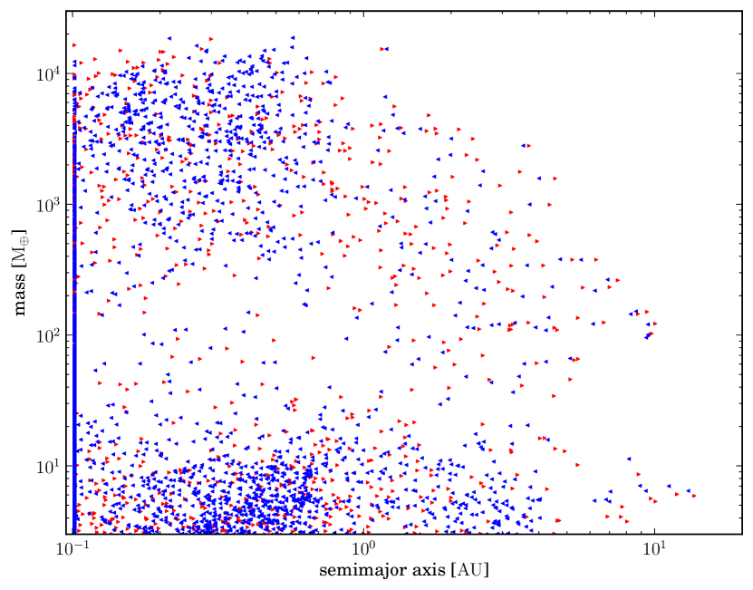
Figure 9: Final position of the planets in the distance - mass diagram. Red, right-facing triangles shows the positions obtained with the isothermal migration model. Blue, left-facing triangles correspond to the reference synthesis.

The first comparison was made with calculations preformed with the nonreduced isothermal migration model ($f_{1}=1$) based on the results of Tanaka et al. (2002). While we used the same type I migration model as in Mordasini et al. (2009a), the results here still differ from those published in Mordasini et al. (2009a), since we here use the same transition criteria for the transition from type I into type II migration as in the reference synthesis. This is different from the one in Mordasini et al. (2009a). There only the thermal condition ($H>R_{\rm H}$) for the transition into type II was used. This leads to much smaller transition masses than here.

Figure 9 shows the final position of the planets in the distance-mass diagram in red, right-facing triangles. Blue, left-facing triangles show the reference synthesis. While the range in mass and distance covered by the planets is the same, there is no clustering caused by the migration into a CZ at small masses (0.6 to 30 $\rm M_{\oplus}$). The total number of “cold” planets ($a>0.1\ AU$) is only $\approx 45\%$ of the number found in the reference calculation. From the 6850 synthetic planets more massive than 0.6 $\rm M_{\oplus}$ we find 79.2% “hot” planets with 2.7% “hot” massive planets and only 20.8 % planets outside of 0.1 AU. Of these, 346 are more massive than 100 $\rm M_{\oplus}$ (5 %). The new nominal nonisothermal migration model in comparison gives twice as many planets that remain outside of 0.1 AU and also almost twice as many massive planets. Some preliminary calculations indicate that this ratio can increase even more with lower values of $\alpha$. The nominal migration model still leads to a loss of more than half of the planets with more than 0.6 $\rm M_{\oplus}$ into the inner part of the disk inside of 0.1 AU and therefore potentially into the star. On the other hand, the new model doubles the number of planets outside of 0.1 AU compared with the isothermal migration model without any arbitrary reduction factor.

4.1.2 Paardekooper et al. 2011 migration model

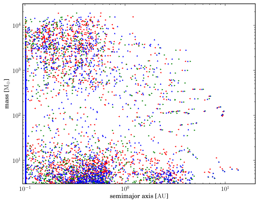
Figure 10: Final position of the planets in the distance-mass diagram. Three different syntheses are shown. Blue, up-facing triangles show the reference synthesis. The other two population calculations are made with the migration model of Paardekooper et al. (2011). Red, left-facing triangles represent planets obtained with this model and the adiabatic coefficient $\gamma$ calculated by our EOS. Green, right-facing triangles show the a-M positions obtained with the Paardekooper et al. 2011 model with a fixed $\gamma=1.4$.

Paardekooper et al. (2011) developed a migration model that is similar to the one described in Section 2, but more sophisticated, because it uses thermal-diffusion time scales and viscous time scales as transition criteria between barotropic and entropy-related parts of the horseshoe drag and the saturation of both. The difference between their and our model are discussed in Section 2.5, where we compared torque curves from our model with those of this model. We also made two synthesis calculations using this migration model. The final a-M distribution of the two simulations is shown in Figure 10. Green dots represent the final positions of the synthetic planets obtained with the Paardekooper et al. (2011) model and a fixed $\gamma=1.4$. The second calculation is shown in red, here $\gamma$ was determined with the EOS we usually use (Saumon et al., 1995). The blue symbols show the reference synthesis.

For planet masses larger than three Earth masses there is no real difference between the three plotted syntheses. The simulation with the free $\gamma$ produces nearly the same number of “cold” planets, the simulation with the fixed $\gamma$ slightly $(5-10\%)$ less relative to the nominal BMF model. The situation is slightly different for the number of massive planets with $M_{\rm p}>100\rm M_{\oplus}$ outside of 1 AU: the free $\gamma$ synthesis has only $85\%$ of the number of “cold” massive planets of the BMF-model synthesis and the fixed-gamma simulation about $60\%$ of the nominal model.

The reason for the small differences in the overall amount of “cold” planets but the larger differences for the “cold” massive planets is, as visible in Fig. 2 and 3, that overall both models produce the same general migration behavior: first planets migrate inward, then outward to a convergence zone, and after saturation inwards again. But the point of crossover from outward to inward migration is closer in and at lower masses for the Paardekooper et al. (2011) model relative to the nominal BMF model. The planets saturate at lower masses and therefore start to rapidly migrate inward earlier in their evolution and fewer planets can reach the type II migration regime and become massive.

Overall, there are no large difference between the different migration models. On the other hand, our simpler BMF model seems to agree better with the torques obtained with the radiative hydrodynamical simulations of Kley et al. (2009) and Bitsch & Kley (2011).

4.2 Different input physics

We now study the effect of different Lindblad torques and of different saturation masses onto the synthetic planet population.

4.2.1 Lindblad torques

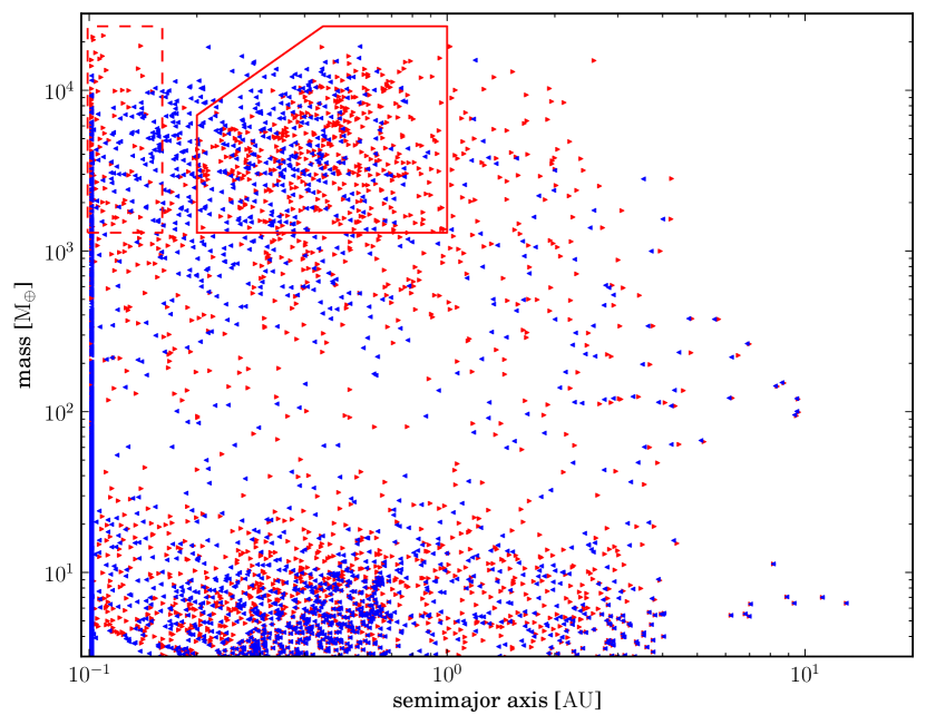
Figure 11: Final position of the planets in the semimajor axis mass diagram. Red shows the final position of planets obtained with the BMF model but with a Lindblad torque formula from Masset & Casoli (2010). In blue are depicted the results of the reference synthesis.

As stated in Section 2.2, there are two different formulas for the Lindblad torques. We changed the Lindblad torque to the one used in Masset & Casoli (2010) for one synthesis. We show the final positions of the planets in the distance-mass diagram in Figure 11. The color-coding is the same as before. The resulting Lindblad torque is weaker with the equation of Masset & Casoli (2010), thus the migration in the saturated regime is slower. This results in moving the high-mass, third clusters farther out. In the reference synthesis the outer cluster is located between 0.1 AU and 0.6 AU. Here, it is located between 0.2 AU and 1 AU (red solid box). Inside of 0.2 AU one can see some planets of a fourth cluster. The planets in this inner group originate in part from fast growing planets, that is, those large dust-to-gas-ratios, of the inner convergence zone. The rest are planets from the outer zone, which saturated but grow rapidly enough during their fast inward-migration phase to transition into type II migration. In contrast to the reference synthesis, where all planets of this group migrated to the inner border of the computational domain at 0.1 AU, the planets are now at larger distances and can be seen in the calculation (red dashed box). The third cluster (outside of 1AU) completely consists of planets in the outer convergence zone.

The smaller torque also results in a smaller and weaker region of inward migration between the CZ. It is small and weak enough that in some cases, planets can drift from the inner into the outer convergence region, because the migration rate is lower than the movement rate of the CZ due to the evolution of the disk (see Sect. 3.3).

For low-mass planets below the saturation mass the differences are smaller between the two syntheses. There are still the two clusters, associated with the two convergence zones.

We can thus conclude that the weaker Lindblad torque results in an shift of the final position of a planet in the distance-mass diagram to the right that is, to larger distances. Because of this we also see more “cold” (increase from 45.6% to 51.2%) and more massive planets relative to the reference synthesis (increase from 9.3% to 12.1%). The calculated migration rate in saturation is only about a factor of 2-3 smaller with the formula of Masset & Casoli (2010) than that of Paardekooper et al. (2010). This seems small compared with the previous reduction of type I migration by a factor of 10-1000. But still, this small change in the description of a part of the torque by a factor of three has observable influence on the distribution of massive planets by up to a factor of 2 in semimajor axis for some cases.

4.2.2 Saturation mass

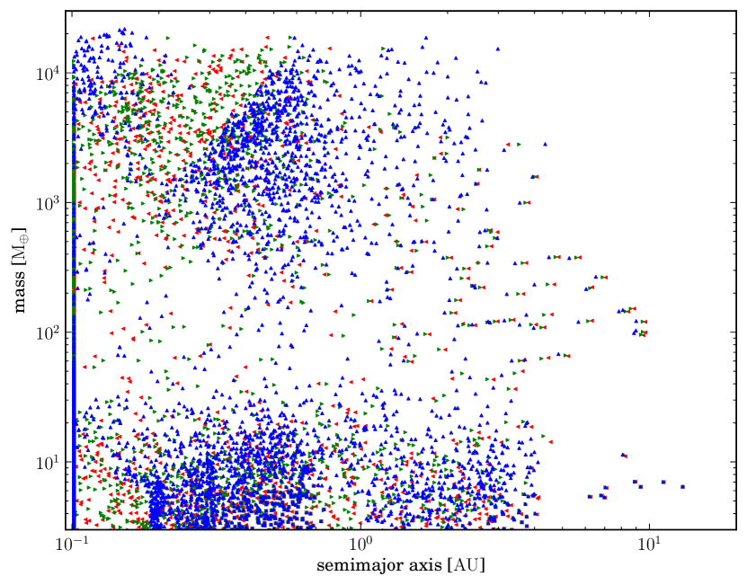
Figure 12: Final position of the planets in the semimajor axis mass diagram. Shown are three different synthesis calculations with different values of $f_{\rm visc}$ and therefore three different saturation mass levels. Red shows the calculation with the largest $f_{\rm visc}$, the STD case. In green is shown the BMF case, and in blue the RED case with the smallest $f_{\rm visc}$.

We furthermore conducted population synthesis calculations with two different values of $f_{\rm visc}$. One with a larger $f_{\rm visc}=1$ (STD model) and one with a smaller $f_{\rm visc}=0.125$ (RED model) than the reference synthesis (BMF model, $f_{\rm visc}=0.55$) (see also 2.6). This only affects planets that are massive enough to undergo the transition into a saturated migration regime. An eight times smaller $f_{\rm visc}$ will result in a four times larger saturation mass (Eq. 28). Figure 12 shows the final positions of the planets in the distance-mass diagram for the two nonnominal calculations and for the reference synthesis. The blue (red) points are the RED (STD) case. For most points of the two clusters of low-mass planets there are only small differences in between these three simulations. They result from the onset of saturation at different masses. For example, some of the planets in these clusters will start to saturate with the STD model while they are still in the unsaturated adiabatic migration regime at the same mass with the RED model and thus migrate faster and also accrete differently because of the different migration rates.

The high-mass clusters are shifted farther out in the synthesis with $f_{\rm visc}=0.125$ than in the reference calculation. Moreover, the fourth group mentioned in Sect. 4.2.1 is visible for planets obtained from the RED case. In this situation the time planets spend in the saturated migration regime is shorter because of the higher saturation mass, therefore the distance they migrate inward is smaller and the planets end up farther out. This has an effect on the content of heavy elements in the planet. Less migration means that the planet can reach less amount of planetesimals in our disk. The difference is the amount of solids in the annulus of the planetesimal disk that is not visited by the planet with the larger saturation mass. But the difference in the final mass for most massive planets ( $>1000\ \rm M_{\oplus}$) is small, lower than $1\%$. The reason is that they grow the most while they are in type II migration and the runaway accretion phase. In this phase the accretion is dominated by gas accretion. Here the growth is set by the remaining disk lifetime, and this is almost the same for the different cases.

Note that we made one simplifying assumption: we included the eccentric instability (Kley & Dirksen, 2006). Therefore gap formation does not lead to a reduction of the planetary gas accretion rate. If this effect were not included, the maximal planet masses would be on the order of 10 Jovian masses (Lubow et al., 1999; Armitage, 2007).

Planets beyond 2 AU and between 60 and $400\ \rm M_{\oplus}$ are closer to the star with a higher saturation mass level than the planets mentioned above. The disk temperature is lower in the outer parts and the slope of the temperature profile begins to become flatter ($\beta_{\rm T}\rightarrow 0$) as the temperature approaches the assumed background temperature of $10\ \rm K$. This change in the slope leads to a strong change in the horseshoe drag at a radius around 10 AU for early disk times and farther in at later times. It dictates the position of the outer convergence zone (Kretke & Lin, 2012). The change of the slope causes the horseshoe drag itself to become negative not far outside of the outer CZ and pushes the planet inward, as does the Lindblad torque. This means that an increase in the saturation mass will result in faster overall inward migration for the planets that start outside the outer CZ and are saturated in this part of the disk.

When comparing the numbers of “cold” planets in the STD and the RED case we see that the increase of the saturation mass by a factor of 4 results in 64% more “cold” planets and also 156% more “cold” massive planets. The number of “hot” massive planets is reduced from 7.5% to 1.4% as the slower overall migration shifts the clusters outward. Even if we cannot directly compare our results with observations, as a reference, Mayor et al. (2011) stated an observational value of $\approx 1\%$.

5 Irradiated vs nonirradiated disks

We recently included irradiation of the host star into the disk model assuming an equilibrium flaring angle (Fouchet et al., 2012). In all calculations presented above, viscous heating only determined the thermal structure of the disk. This is sufficient in the inner parts of the disk at the beginning of the simulations, but leads to too low temperatures in the outer parts of the disk and in the later phases of the disk evolution, when the rate of gas flow through the disk becomes low and the irradiation is dominant. This effect leads to a different temperature gradient, which is important for the strength of the torques (Lyra et al., 2010). The increased heating in the outer parts makes the temperature profile less steep throughout the disk. The temperature is still around $20\ \rm K$ at $50\ \rm AU$ and decreases with distance, while in the nonirradiated case the temperature dropped to the background temperature of $10\ \rm K$ at $20-30\ \rm AU$ and became nearly constant. The temperature structure in the whole disk is set only by the irradiation when the disk is nearly gone and viscous heating is unimportant for the temperature structure of the entire disk. The different profile also affects the shape of the convergence regions. The parts of inward migration in the disk become smaller with time and vanish after a few million years, but still before the disk dissolves (Kretke & Lin, 2012). This affects first the outer and then the inner CZ. Thus, the CZ is no longer a stopping point for type I migration throughout the complete lifetime of a disk. Therefore the confinement of planets in a small radius (see Appendix A) even when only one value of the photoevaporation rate is used is not the case for irradiated disks.

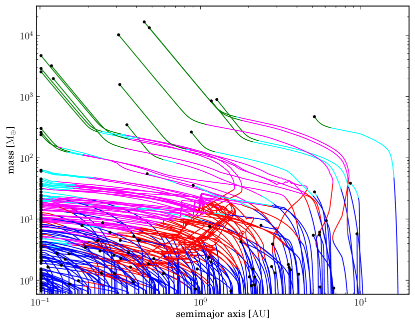
Figure 13: Formation tracks for 250 planets of a synthesis with an irradiated disk model. The meaning of the colors is the same as in Fig. 7.

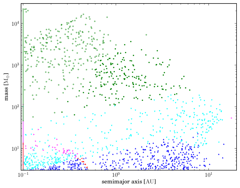
Figure 14: Final position of the planets in the semimajor axis mass diagram in the disks including stellar irradiation. The bars at 0.1 AU indicate the mass range of the “hot” planets in the different regimes. The meaning of the colors is the same as in Fig. 7. Filled (empty) symbols represent planets that never (sometime) migrated in their evolution in an adiabatic migration regime.

Figure 13 shows the formation tracks of 250 initial conditions and Figure 14 shows the final positions of the planets in the distance-mass diagram. In both figures color shows the different migration regimes a planet is in in the same ways as in Figure 7. The different symbols in Figure 14 indicate if a planet migrated in adiabatic regime during its evolution (empty triangles or circle) or not (filled triangles or circle). The new temperature structure and increase in temperature results in a switch into the adiabatic migration regime at a higher mass than in the nonirradiated disk calculations. Moreovre, as seen in these figures, almost all small planets end in a locally isothermal migration regime even when they went into the adiabatic regime for some part of their evolution (as shown by the red part of the tracks in Figure 13) and the unfilled cyan triangles in Fig. 14, they end in a locally isothermal regime again when the disk is almost gone. The higher temperature than in the one in nonirradiated disks, especially at the end when almost all gas is gone and only minor viscous heating occurs, leads to a shorter cooling time and therefore to the transition from adiabatic migration into locally isothermal migration.

The irradiation also leads to higher disk accretion rates in the outer regions of the disk, since $\nu=\alpha c_{\rm s}\texttwosuperior/\Omega\propto T$, and therefore to the faster depletion of the outer disk regions. The surface density is therefore lower in the irradiation case than in the nonirradiated at same time of the simulation. This leads to lower migration rates even in locally isothermal migration. This compensates to some degree the larger inward migration zones in our disks and the transition into locally isothermal migration at the end of the disk lifetime.

We used the same initial conditions as in all other syntheses. The different disk model leads to different disk lifetimes, therefore the results are only partially comparable. We considered 7700 planets more massive than $0.6\ \rm M_{\oplus}$. From these planets $68.8\%$ migrated to the inner border of our computational domain. From the planets with a final distance larger than 0.1 AU from the star $\approx 20\%$ are more massive than $100\ \rm M_{\oplus}$, which is similar to the ratio in our reference synthesis. The larger amount of “hot” planets is the result from the disappearing CZs at toward end of the disk evolution.

6 Summary and conclusions

We have compiled a prescription for type I migration based on the latest hydrodynamic simulations of planet-disk interactions. We tested the influence of the prescription on the outcome of the planetary population synthesis calculations. Our migration model is based on the combination of results from Paardekooper et al. (2010) and different time scales to distinguish between different migration regimes. These time scales reflect the thermodynamical behavior of the interaction between the planet and the surrounding disk like the horseshoe drag. We first compared the migration torques of this model with a model of Paardekooper et al. (2011) and with radiative-hydrodynamical simulations from Kley et al. (2009) and Bitsch & Kley (2011). The comparison of the theoretical torque curves with data from Kley et al. (2009) and Bitsch & Kley (2011) suggests that with an adjustment of the viscous time scale in the calculation of the saturation mass (the mass when the corotation torque starts to vanish) by a factor of $f_{\rm visc}\approx 0.55$ our model reproduces the torque better.

We also showed the global effects of different parameters of various migration models in a number of population synthesis calculations. Here, the comparison of our nominal BMF model ($f_{\rm visc}\approx 0.55$) and the migration model of Paardekooper et al. (2011) indicates similar results (Sect. 4.2.2) even with the difference shown in the torque curves.

Like Lyra et al. (2010),Kretke & Lin (2012), and Hellary & Nelson (2012), we also find with our prescription that nonisothermal type I migration leads to convergence zones (CZ), that is, points in a disk to which planets migrate to from the inside and outside. As in previous studies (Hellary & Nelson, 2012), we find that the convergence zones move inward as the disk evolves and take the captured planets with it. This occurs on the slower time scale of disk evolution and therefore the captured planets are trapped in it and also only migrate on this time scale. The planets leave this zone when their horseshoe drag saturates.

The difference between the migration rate of planets captured in a CZ and the migration rate in the saturated regime is significant. This means that an increase of the mass where saturation occurs by a modest factor of 2, for example, the time spent in rapid-saturated type I migration is significantly shortened and therefore also the extent of migration. The level of saturation at a given mass, and the mass at which saturation begins, are among the critical aspects for the evolution of a giant planet since small changes by a factor of 2 in $f_{\rm visc}$ can change the final distribution in the mass semimajor axis diagram by a measurable degree. But a similar degree of change in the final semimajor axis-mass distribution was seen when we changed the description of the Lindblad torque to the formula found by Masset & Casoli (2010).

Finally, we determined the formation tracks of a planet, illustrating that under certain conditions, a planet can loose almost all of its gas mass during its evolution. This mass loss can lead to a stop of migration for a few $10^{5}$ years when the mass loss is strong enough to desaturate the horseshoe drag. The reason for the envelope mass loss is a jump in solid accretion rate, which is caused by the migration of the planet from a solid-depleted into a solid-rich region of the disk. This behavior strongly depends on the treatment of the planetesimal disk. Here we did not evolve the disk or changed the random velocities because of a giant planet. Both change the accretion rate and therefore whether or how this mass loss occurs.

Neither did we consider random variations in the torque due to turbulent density variations in the disk. Recent studies showed that in some cases random migration due to turbulence can dominate the migration behavior for low-mass planets (Papaloizou et al., 2004; Uribe et al., 2011). Depending on the strength of the random torque, it could push planets from the inner into the outer convergence zone even for the stronger Lindblad torque of Paardekooper et al. (2011).

We made no detailed comparison with observed extrasolar planet populations because the migration model is only a small part of the improvements to the overall model, and defer such comparisons to future work. But we quantified the impact of different model settings by studying the fractional yield of different planet types in a synthesis.

With the new nonisothermal migration model described here or that of Paardekooper et al. (2011) there are still about $50\%$ of all low-mass planets lost in the innermost part of the disk. However, it is about a factor two better than the isothermal migration model without any artificial factors. One way to reduce the number of “lost” planets is an increase of the saturation mass. A lower critical mass for runaway gas accretion can also help due to the faster transition into type II migration (Hori & Ikoma, 2011). Furthermore, there are hints that there are additional effects leading to outward migration of planets in 3D simulations of magneto-hydrodynamic disks (Uribe et al., 2011).

We also note that up to now there is a shortcoming of all analytic torque predictions: they all neglect the fact that the horseshoe region is over-wide compared with the prediction used here when $q/h^{3}\approx 1$ (Masset et al. (2006)). The fast growth of the width of the horseshoe region in that mass range (a few ten Earth masses to a hundred Earth masses) yields a boost of the corotation torque, which is a strong effect. In the same mass range gap opening and the transition into type II migration occur. And as shown in Section 2.5, saturation plays a main role in the change of the direction of the torque in that mass range as well. Moreover, our fit of the torques data from Kley et al. (2009) and Bitsch & Kley (2011) depends on the progression of the torque curve in that mass range. This means that even when our fit produced the torque data well, a closer study of the torque in the mass range might uncover new effects, that may change the outcome of population synthesis calculations.

Nevertheless, the CZ or a similar effect might explain the concentration of planets in clusters one finds in distance-mass diagrams of observed extrasolar planets for high- and low-mass planets (Mayor et al., 2011). In particular, the absence of close-in, low-mass planets in Mordasini et al. (2009b) is not seen any longer with the updated migration model.

Additional comparisons of our results with new data from radial velocity measurements and Kepler data will be important, especially when we combine the new migration model with new improvements of our model, i.e., the long term evolution of giant planets (Mordasini et al., 2012b) and the concurring evolution of multiple planets per disk (Ida & Lin, 2010; Alibert et al., 2013). Multiple cores in one disk might be collected into one CZ and form one larger core. Therefore the convergence region may function as a large feeding zone of solid matter onto a core captured in a convergence zone and thus enhance the solid accretion rate (Hellary & Nelson, 2012; Sándor et al., 2011; Horn et al., 2012). Moreover, in particular the low-mass planets of the inner cluster only migrated through the inner convergence region. The outer boundary of this region is due to the transition in the gas opacity at the iceline. This means that all these planets moved only through the ice-free part of the protoplanetary disk. We will also study the global effects of different viscous $\alpha$ values and deadzones on the behavior of the convergences zones with population synthesis calculations (cf. Hasegawa & Pudritz, 2011). This brings us closer to a description of orbital migration without ad hoc efficiency factors.

Appendix A Saturation and disk evolution

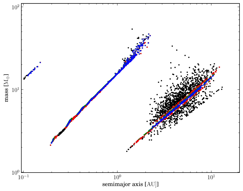
Figure 15: Position of a planet in the nominal synthesis calculation when it transitions from the unsaturated adiabatic migration regime into the saturated adiabatic migration regime. Colored are the planet which distance is less than 3% (blue, up facing triangles), 5% (green, right facing triangles) or 10% (red, left facing triangles) from a CZ.

From the positions of planets at the time of saturation in the formation tracks in Figure 7 in Section 3.5 one sees that most positions lie on two lines, one for the planets of the inner and one for the outer CZ. We study here the reasons for this feature.

Figure 15 shows the positions of the planets at the transition from unsaturated to saturated adiabatic migration, the most common transition into a saturated migration regime. The positions of all planets undergoing this transition are shown in black, while the colored points show that those with a distance between their semimajor axis and the position of the CZ at that time are fewer than 10% of the semimajor axis. There are two large groups, again one of the inner and one of the outer convergence region. Almost all planets of the inner group are in the CZ when they saturate, while the outer ones are much more spread out. But the planets that are in the CZ form a line here as well. There is a third CZ inside of 0.3 AU in the most massive disks in the synthesis, which leads to a third minor group. However, this CZ evolves quickly and disappears after the first few 0.01 Myr and all associated planets end at 0.1 AU. The dozen points inside of 0.2 AU in Fig. 15 correspond to planets in this small CZ.

This behavior results from the interaction of the following points:

One can calculate the saturation mass as a function of the orbital distance $a$ and time $t$ by setting $s_{2}=1$ in Eq. 17. There, $f_{\rm visc}$ is 1, 0.55 or 0.125 in each of the model versions.

$$M_{\rm sat}(a,t)=\frac{h(a,t)}{1.16}\left(\frac{8\pi M_{*}\nu(a,t)}{3f_{\rm visc}}\right)^{\frac{2}{3}}\frac{1}{(Ga)^{1/3}}.$$ (28)

For a fixed orbital distance and stellar mass it only depends on the disk aspect ratio $h$ and the viscosity $\nu$. Both quantities are decreasing with time, as the disk mass decreases, and therefore, the saturation mass also becomes smaller as the disk evolves.

While the photoevaporation rate is important for the lifetime of a disk, the constant value of $\alpha$ in all simulations of one synthesis results in a similar disk structure in the part of the disk where viscosity is dominant. There, the disks go through the same series of disk states (radial profile of temperature, surface density, etc.) and only the speed with which the disks go through the states is different and depends on the photoevaporation rate. Given one semimajor axis $a$, there is only one disk state where the inner (our outer) CZ lie at this position. Therefore also $h$ and $\nu$ are fixed for this semimajor axis of the CZ. Therefore, the semimajor axis of the CZ corresponds to only one saturation mass. And as the CZ moves inward while the disk evolves, the saturation mass decreases. Both processes approximately follow power-laws and thus we see a line-like structure for the planets that saturate while they are in one CZ. Planets that saturate early in the disk evolution do so at a higher mass and farther out than planets that saturate in later times of disk evolution.

Finally, the spread in the outer group results from planets that saturated before they reached the CZ. These are planets in disks with high solid surface densities where the planet cores can grow fast. Compared with the inner group, the outer group also contains more planets that saturate outside of the CZ. The larger amount of solids outside of the iceline leads to higher accretion rates. The scatter is reduced when the saturation mass is increased by reducing $f_{\rm visc}$. The higher saturation mass gives the planets more time to migrate to the CZ and to saturate there.

Appendix B Impact of numerical parameters

We made several population syntheses calculation to test the effects of different numerical parameters and comment on the effects here.

We made calculations with the STD model and exponents $b=2.0$ and $b=10.0$ (nominal value $b=4.0$) in the transition function between locally isothermal and adiabatic migration regime (Eq. 20). This only has a small effect for low-mass planets, while for massive planets the final semimajor axis and mass is almost the same for different values of $b$. At smaller masses no clear pattern can be seen. An increase of $b$ can lead to either more or less massive planets and to either larger or smaller distances from the star of a few per cent.

We also made calculations with $b=4.0$ and a hard jump for the transition function between type I and type II migration (Eq. 23) (nominal value $b=10$. This only affects massive planets and gives only a change in distance from the star of a few percent, with a larger $b$ leading to planets farther away from the star but almost no change in the final mass.

Overall, the range of the different parameters studied here only leads to minor changes in the overall distribution of planets in semimajor axis and mass.

References

- Alexander & Armitage (2009) Alexander, R. D. & Armitage, P. J. 2009, ApJ, 704, 989
- Alibert et al. (2013) Alibert, Y., Carron, F., & Fortier, A. 2013, A&A, in review
- Alibert et al. (2004) Alibert, Y., Mordasini, C., & Benz, W. 2004, A&A, 417, L25
- Alibert et al. (2011) Alibert, Y., Mordasini, C., & Benz, W. 2011, A&A, 526, A63
- Alibert et al. (2005) Alibert, Y., Mordasini, C., Benz, W., & Winisdoerffer, C. 2005, A&A, 434, 343
- Armitage (2007) Armitage, P. J. 2007, The Astrophysical Journal, 665, 1381
- Armitage & Rice (2005) Armitage, P. J. & Rice, W. K. M. 2005, STScI Symposium A Decade Of Extrasolar Planets Around Normal Stars
- Baruteau & Masset (2008) Baruteau, C. & Masset, F. 2008, ApJ, 672, 1054
- Batalha et al. (2011) Batalha, N. M., Borucki, W. J., Bryson, S. T., et al. 2011, ApJ, 729, 27
- Bell & Lin (1994) Bell, K. R. & Lin, D. N. C. 1994, ApJ, 427, 987
- Bitsch & Kley (2011) Bitsch, B. & Kley, W. 2011, A&A, 536, A77
- Bodenheimer et al. (2013) Bodenheimer, P., D’Angelo, G., Lissauer, J. J., Fortney, J. J., & Saumon, D. 2013, ApJ, 770, 120
- Casoli & Masset (2009) Casoli, J. & Masset, F. S. 2009, ApJ, 703, 845
- Crida & Morbidelli (2007) Crida, A. & Morbidelli, A. 2007, MNRAS, 377, 1324
- Crida et al. (2007) Crida, A., Morbidelli, A., & Masset, F. 2007, A&A, 461, 1173
- D’Angelo et al. (2002) D’Angelo, G., Henning, T., & Kley, W. 2002, A&A, 385, 647
- Fortier et al. (2013) Fortier, A., Alibert, Y., Carron, F., Benz, W., & Dittkrist, K.-M. 2013, A&A, 549, A44
- Fortier et al. (2007) Fortier, A., Benvenuto, O. G., & Brunini, A. 2007, A&A, 473, 311
- Fouchet et al. (2012) Fouchet, L., Alibert, Y., Mordasini, C., & Benz, W. 2012, A&A, 540, A107
- Goldreich & Tremaine (1980) Goldreich, P. & Tremaine, S. 1980, ApJ, 241, 425
- Guilet et al. (2013) Guilet, J., Baruteau, C., & Papaloizou, J. C. B. 2013, MNRAS, 430, 1764
- Hasegawa & Pudritz (2011) Hasegawa, Y. & Pudritz, R. E. 2011, MNRAS, 417, 1236
- Hellary & Nelson (2012) Hellary, P. & Nelson, R. P. 2012, MNRAS, 419, 2737
- Hori & Ikoma (2011) Hori, Y. & Ikoma, M. 2011, MNRAS, 416, 1419
- Horn et al. (2012) Horn, B., Lyra, W., Mac Low, M.-M., & Sándor, Z. 2012, ApJ, 750, 34
- Ida & Lin (2004) Ida, S. & Lin, D. N. C. 2004, ApJ, 604, 388
- Ida & Lin (2008) Ida, S. & Lin, D. N. C. 2008, ApJ, 673, 487
- Ida & Lin (2010) Ida, S. & Lin, D. N. C. 2010, ApJ, 719, 810
- Kley et al. (2009) Kley, W., Bitsch, B., & Klahr, H. 2009, A&A, 506, 971
- Kley & Dirksen (2006) Kley, W. & Dirksen, G. 2006, A&A, 447, 369
- Kretke & Lin (2012) Kretke, K. A. & Lin, D. N. C. 2012, ApJ, 755, 74
- Lubow et al. (1999) Lubow, S. H., Seibert, M., & Artymowicz, P. 1999, ApJ, 526, 1001
- Lynden-Bell & Pringle (1974) Lynden-Bell, D. & Pringle, J. E. 1974, MNRAS, 168, 603
- Lyra et al. (2010) Lyra, W., Paardekooper, S., & Mac Low, M. 2010, ApJ, 715, L68
- Marois et al. (2008) Marois, C., Macintosh, B., Barman, T., et al. 2008, Science, 322, 1348
- Masset (2002) Masset, F. S. 2002, A&A, 387, 605
- Masset & Casoli (2009) Masset, F. S. & Casoli, J. 2009, ApJ, 703, 857
- Masset & Casoli (2010) Masset, F. S. & Casoli, J. 2010, ApJ, 723, 1393
- Masset et al. (2006) Masset, F. S., D’Angelo, G., & Kley, W. 2006, ApJ, 652, 730
- Mayor et al. (2011) Mayor, M., Marmier, M., Lovis, C., et al. 2011, ArXiv e-prints, 1109.2497
- Miguel & Brunini (2008) Miguel, Y. & Brunini, A. 2008, MNRAS, 387, 463
- Mizuno et al. (1978) Mizuno, H., Nakazawa, K., & Hayashi, C. 1978, Progress of Theoretical Physics, 60, 699
- Mordasini et al. (2009a) Mordasini, C., Alibert, Y., & Benz, W. 2009a, A&A, 501, 1139
- Mordasini et al. (2009b) Mordasini, C., Alibert, Y., Benz, W., & Naef, D. 2009b, A&A, 501, 1161
- Mordasini et al. (2012a) Mordasini, C., Alibert, Y., Georgy, C., et al. 2012a, A&A, 547, A112
- Mordasini et al. (2012b) Mordasini, C., Alibert, Y., Klahr, H., & Henning, T. 2012b, A&A, 547, A111
- Mordasini et al. (2011) Mordasini, C., Dittkrist, K.-M., Alibert, Y., et al. 2011, in IAU Symposium, Vol. 276, IAU Symposium, ed. A. Sozzetti, M. G. Lattanzi, & A. P. Boss, 72–75
- Mordasini et al. (2010) Mordasini, C., Klahr, H., Alibert, Y., Benz, W., & Dittkrist, K.-M. 2010, in Circumstellar Disks and Planets: Science Cases for the Second Generation VLTI Instrumentation, ed. S. Wolf, [arXiv:1012.5281]
- Nagasawa et al. (2008) Nagasawa, M., Ida, S., & Bessho, T. 2008, ApJ, 678, 498