A Multiplierless Pruned DCT-like Transformation for Image and Video Compression that Requires 10 Additions Only

Abstract

A multiplierless pruned approximate 8-point discrete cosine transform (DCT) requiring only 10 additions is introduced. The proposed algorithm was assessed in image and video compression, showing competitive performance with state-of-the-art methods. Digital synthesis in 45 nm CMOS technology up to place-and-route level indicates clock speed of 288 MHz at a 1.1 V supply. The $8\times 8$ block rate is 36 MHz. The DCT approximation was embedded into HEVC reference software; resulting video frames, at up to 327 Hz for 8-bit RGB HEVC, presented negligible image degradation.

Keywords
Approximate discrete cosine transform, pruning, pruned DCT, HEVC

1 Introduction

The discrete cosine transform (DCT) plays a fundamental role in signal processing techniques [1] and is part of modern image and video standards, such as JPEG [2], MPEG-1 [3], MPEG-2 [4], H.261 [5], H.263 [6], H.264/AVC [7, 8], and the high efficiency video coding (HEVC) [9, 10]. In particular, the transform coding stage of the H.264 and HEVC standards employs the 8-point DCT of type II [10, 11] among other transforms of different blocklenghts, such as 4, 16, and 32 points [12, 13, 14]. In [15], the 8-point DCT stage of the HEVC was optimized. Among the above-mentioned standards, the HEVC is capable of achieving high compression performance at approximately half the bit rate required by H.264/AVC with same image quality [10, 13, 16, 15]. However, HEVC possesses a significant computational complexity in terms of arithmetic operations [13, 16, 11, 15]. In fact, HEVC can be 2–4 times more computationally demanding when compared to H.264/AVC [13, 15]. Therefore, the proposal of efficient low-complexity DCT-like approximations can benefit future video codecs including emerging HEVC-based systems.

Recently, low-complexity DCT approximations have been considered for image and video processing [17, 18, 19, 20, 21, 22, 15, 12, 23, 24]. Such approximate transforms can offer meaningful DCT estimations at the expense of small errors. Such trade-off is often acceptable leading to low-power, high-speed hardware realizations [15], while ensuring adequate numerical accuracy.

In some applications, such as data compression [25], high-frequency components are often zeroed by the quantization process. Thus, one may judiciously restrict the computation to the quantities that are likely to be remain significant [26]. This approach is called pruning and was originally proposed as a method for computing the discrete Fourier transform (DFT) [27, 28].

1.1 Related Works

In that context, pruning was applied in time-domain, i.e., particular input samples were ignored and the operations involving them were avoided [29]. Frequency-domain pruning—discarding transform coefficients—is an alternative approach. This latter approach has been recently applied in mixed-radix FFT algorithms [30], cognitive radio design [31], and wireless communications [32]. Another example of a pruning-like algorithm is the well-known Goertzel method for DFT computation [33, 34, 35].

For the DCT case, pruning was originally proposed by Wang in [36] considering a decimation-in-time algorithm for power-of-two blocklengths. In [37], such algorithm was generalized for arbitrary blocklength. In [38], Lecuire et al. extended the pruning method to the two-dimensional case, referring to the method as the zonal DCT, which is an alternative terminology. In [39], Karakonstantis et al. proposed a hardware-based pruning approach for the DCT computation. Instead of discarding high frequency DCT coefficients, a VLSI system capable of computing low frequency components using faster paths was suggested. Such method was applied in the context of voltage scaling for low-power dissipation. In the context of low-powered wireless vision sensor networks, a pruned approximate DCT was proposed in [40] based on the DCT approximation theory advanced in [20]. In [41] the pruning terminology was employed in a different context. It was considered to describe a hardware computation of the DCT which maintains the system word size constant by means of a controlled discarding of least-significant bits.

1.2 Aims

In response to the growing need for high compression ratios for image and moving pictures as prescribed in [9], we propose a further reduction of the computational cost of the DCT computation in the context of JPEG- and HEVC-like coding and processing. The goal of this paper is to offer a comprehensive analysis of pruning schemes in combination with approximate transforms. The sough schemes must be capable of reducing the number of computed approximate DCT coefficients and, at the same time, the effected degradation on picture quality must be negligible.

In the present work, a multiplication-free pruned approximate 8-point DCT is sought. We also aim at VLSI realizations of both 1-D and 2-D versions of the proposed pruned approximate transform. The sought methods are intended to be fully embedded into an open source HEVC reference software [42] for performance assessment in real time video coding.

2 Proposed pruned approximate DCT

2.1 Proposed approximation

In [22] a very low-complexity 8-point DCT approximation was introduced and it is referred to as the modified rounded DCT (RDCT), which is associated to the following low-complexity matrix:

$$\bm{T}=\left[\begin{array}[]{rrrrrrrr}1&\phantom{-}1&1&1&1&\phantom{-}1&\phantom{-}1&1\\ 1&0&0&0&0&0&0&-1\\ 1&0&0&-1&-1&0&0&1\\ 0&0&-1&0&0&1&0&0\\ 1&-1&-1&1&1&-1&-1&1\\ 0&-1&0&0&0&0&1&0\\ 0&-1&1&0&0&1&-1&0\\ 0&0&0&-1&1&0&0&0\end{array}\right].$$ (9)

Its associated fast algorithm requires only 14 additions, having the lowest computational complexity among the meaningful DCT approximations archived in literature [43, 17, 18, 19, 20, 21, 22, 15]. Considering the orthogonalization methods described in [44], an orthonormal approximation for the DCT is given by given by:

$$\hat{\bm{C}}=\bm{D}\cdot\bm{T}=\frac{1}{2}\cdot\operatorname{diag}\left(\frac{1}{\sqrt{2}},\sqrt{2},1,\sqrt{2},\frac{1}{\sqrt{2}},\sqrt{2},1,\sqrt{2},\right)\cdot\bm{T},$$ (10)

where $\operatorname{diag}(\cdot)$ returns a diagonal matrix with the elements of its argument.

By means of analyzing fifty 512$\times$512 8-bit representative standard images [45], we noticed that the 2-D version of the 8-point modified RDCT [22] can concentrate in average $\approx$98% of the total image energy in the 16 lower frequency coefficients. Additionally, in JPEG-like image compression, the quantization step is prone to zero the high frequency coefficients [38]. Therefore, computational efforts may be saved by not computing the high frequency coefficients, keeping only low-frequency coefficients. These considerations yield the following transformation derived from the low-complexity matrix associated to the modified RDCT:

$$\bm{T}_{4}=\left[\begin{array}[]{rrrrrrrr}1&\phantom{-}1&1&1&1&\phantom{-}1&\phantom{-}1&1\\ 1&0&0&0&0&0&0&-1\\ 1&0&0&-1&-1&0&0&1\\ 0&0&-1&0&0&1&0&0\\ \end{array}\right].$$ (15)

Above transformation computes the four lower frequency components of the 1-D original modified RDCT low-complexity matrix, which corresponds to the 16 lower frequency components of the associated 2-D version. Thus, considering the orthogonalization methods described in [44], we can obtain a semi-orthogonal matrix given by:

$$\hat{\bm{C}}_{4}=\bm{D}_{4}\cdot\bm{T}_{4}=\frac{1}{2}\cdot\operatorname{diag}\left(\frac{1}{\sqrt{2}},\sqrt{2},1,\sqrt{2}\right)\cdot\bm{T}_{4}.$$ (16)

Matrix $\hat{\bm{C}}_{4}$ is the pruned version of the modified RDCT. For image and video compression, the scaling diagonal matrix $\bm{D}_{4}$ does not introduce any computational overhead, since it can be merged into the quantization step [18, 19, 21, 22, 15]. Therefore, in such context, the computational complexity of $\hat{\bm{C}}_{4}$ is essentially confined into the low-complexity matrix $\bm{T}_{4}$. Aiming at the efficient of implementation of $\bm{T}_{4}$, we factorized it in a product of extremely low-complexity sparse matrices. Such factorization is based on decimation-in-time methods as described in [46, 43, 21]. Thus, the following expression is obtained:

$$\bm{T}_{4}= \bm{P}\cdot\bm{A}_{3}\cdot\bm{A}_{2}\cdot\bm{A}_{1},$$ (17)

where

$$\begin{split}\bm{P}&=\begin{bmatrix}1&0&0&0\\ 0&0&0&1\\ 0&1&0&0\\ 0&0&1&0\end{bmatrix},\\ \bm{A}_{3}&=\begin{bmatrix}1&1&0&0&0\\ 0&0&1&0&0\\ 0&0&0&1&0\\ 0&0&0&0&1\end{bmatrix},\\ \bm{A}_{2}&=\begin{bmatrix}1&\phantom{-}0&\phantom{-}0&\phantom{-}1&\phantom{-}0&\phantom{-}0\\ 0&\phantom{-}1&\phantom{-}1&\phantom{-}0&\phantom{-}0&\phantom{-}0\\ 1&\phantom{-}0&\phantom{-}0&-1&\phantom{-}0&\phantom{-}0\\ 0&\phantom{-}0&\phantom{-}0&\phantom{-}0&-1&\phantom{-}0\\ 0&\phantom{-}0&\phantom{-}0&\phantom{-}0&\phantom{-}0&\phantom{-}1\end{bmatrix},\\ \bm{A}_{1}&=\begin{bmatrix}1&\phantom{-}0&\phantom{-}0&\phantom{-}0&\phantom{-}0&\phantom{-}0&\phantom{-}0&\phantom{-}1\\ 0&\phantom{-}1&\phantom{-}0&\phantom{-}0&\phantom{-}0&\phantom{-}0&\phantom{-}1&\phantom{-}0\\ 0&\phantom{-}0&\phantom{-}1&\phantom{-}0&\phantom{-}0&\phantom{-}1&\phantom{-}0&\phantom{-}0\\ 0&\phantom{-}0&\phantom{-}0&\phantom{-}1&\phantom{-}1&\phantom{-}0&\phantom{-}0&\phantom{-}0\\ 0&\phantom{-}0&\phantom{-}1&\phantom{-}0&\phantom{-}0&-1&\phantom{-}0&\phantom{-}0\\ 1&\phantom{-}0&\phantom{-}0&\phantom{-}0&\phantom{-}0&\phantom{-}0&\phantom{-}0&-1\end{bmatrix},\end{split}$$ (18)

where $\bm{A}_{1}$, $\bm{A}_{2}$, and $\bm{A}_{3}$, are pre-addition matrices [46] and $\bm{P}$ is a permutation matrix. Fig. 1 provides the signal flow graph of the fast algorithm for $\bm{T}_{4}$, relating input signal $x_{n}$, $n=0,1,\ldots,7$ to output signal $X_{k}$, $k=0,1,\ldots,7$. Transform-domain components $X_{4},\ldots,X_{7}$ are not represented, being set to zero.

Based on the 2-D computation of the DCT [43], the approximate 2-D DCT is given by [18]:

$$\bm{B}=\hat{\bm{C}}\cdot\bm{A}\cdot\hat{\bm{C}}^{\top},$$ (19)

where $\bm{A}$ is an input 8$\times$8 image subblock, $\bm{B}$ is the associated transform-domain 8$\times$8 output image subblock and superscript $\top$ indicates matrix transposition. For instance, JPEG-like schemes are entirely based on the DCT-based transformation of 8$\times$8 subblocks [2].

In a similar fashion, the 2-D forward pruned transformation can be derived [47, 38, 40] and it is described according to:

$$\bm{B}^{\prime}=\hat{\bm{C}}_{4}\cdot\bm{A}\cdot\hat{\bm{C}}_{4}^{\top},$$ (20)

where $\bm{B}^{\prime}$ is the pruned 4$\times$4 output image subblock.

Matrix $\bm{B}^{\prime}$ contains a subset of the transform-domain coefficients $\bm{B}$ furnished by the modified RDCT. The approximate 2-D spectrum is given by the 8$\times$8 matrix $\hat{\bm{B}}$ constituted of $\bm{B}^{\prime}$ in upper-left corner and zeros elsewhere, as shown below:

$$\bm{B}\approx\hat{\bm{B}}=\left[\begin{array}[]{c|c}\bm{B}^{\prime}&\bm{0}_{4}\\ \hline\cr\bm{0}_{4}&\bm{0}_{4}\end{array}\right],$$ (23)

where $\bm{0}_{4}$ represents the 4$\times$4 null matrix. The inverse transformation can be computed by taking the inverse transformation of the above zero-padded matrix $\hat{\bm{B}}$. However, this is equivalent to the following computation:

$$\bm{A}\approx\hat{\bm{A}}=\hat{\bm{C}}_{4}^{\top}\cdot\bm{B}^{\prime}\cdot\hat{\bm{C}}_{4}.$$ (24)

Therefore, padding becomes unnecessary. Additionally, we noticed that $\hat{\bm{C}}_{4}^{\top}$ is the Moore-Penrose pseudo-inverse of $\hat{\bm{C}}_{4}$ [48].

Figure 1: Signal flow graph relating input data $x_{n}$, $n=0,1,\ldots,7$, to output $X_{k}$, $k=0,1,3,4$, according to $\bm{T}_{4}$. Dashed arrows are multiplications by $-1$

2.2 Complexity Assessment

By counting the number of multiplications, additions, and bit-shifting operations, we assessed the computational cost of the proposed 1-D and 2-D pruned modified RDCT. Table 1 compares the obtained complexities with the computational costs associated to traditional and state-of-the-art DCT methods. Selected DCT approximations include: (i) the signed DCT (SDCT) [17]; (ii) the rounded DCT (RDCT) [21]; (iii) the modified RDCT [22]; and a set of DCT approximations introduced by Bouguezel-Ahmad-Swamy, namely, BAS-2008 [18], BAS-2009 [19], and BAS-2013 [20]. Here, we also included the computational cost of the exact DCT computation according to Chen’s DCT algorithm [49], which is the algorithm employed in the HEVC codec [42]. Each of the selected methods was assessed both in its full and pruned versions. The 1-D and 2-D versions retained the four and 16 lower frequency coefficients, respectively.

Table 1: Computational complexity assessment

	Nonpruned			Pruned
1-D Method	Mult.	Add.	Shift	Mult.	Add.	Shift
DCT (by definition)	64	56	0	32	28	0
Chen’s DCT [49]	16	26	0	6	12	0
SDCT [17]	0	24	0	0	20	0
BAS-2008 [18]	0	18	2	0	14	1
BAS-2009 [19]	0	18	0	0	14	0
BAS-2013 [20, 40]	0	24	0	0	20	0
RDCT [21]	0	22	0	0	16	0
Modified RDCT [22]	0	14	0	0	10	0
2-D Method	Mult.	Add.	Shift	Mult.	Add.	Shift
DCT (by definition)	1024	896	0	384	336	0
Chen’s DCT [49]	256	416	0	72	144	0
SDCT [17]	0	384	0	0	240	0
BAS-2008 [18]	0	288	32	0	168	12
BAS-2009 [19]	0	288	0	0	168	0
BAS-2013 [20, 40]	0	384	0	0	240	0
RDCT [21]	0	352	0	0	192	0
Modified RDCT [22]	0	224	0	0	120	0

The proposed 1-D method demands only 10 additions. The associate percent complexity reduction compared to selected state-of-art methods is presented in Table 2, for both the 1-D and 2-D case. A certain arithmetic complexity reduction was already expected by using pruning approach. However, when considering the 2-D transformation, arithmetic complexity reduction effected by the pruning procedure is even more significant, as shown in Table 2. In fact, the 8$\times$8 nonpruned 2-D transformation can be decomposed into eight nonpruned row-wise 1-D transformations; followed by eight column-wise instantiations of the same 1-D transformation. In contrast, the proposed pruned 2-D transformation can be decomposed into eight pruned row-wise 1-D transformations of the rows; followed by only four pruned 1-D transformations. Therefore, the pruned 2-D transformation calls the 1-D algorithm fewer times when compared with the nonpruned case. The complexity values presented in Table 1 were calculated according to above considerations. As a consequence, the proposed transformation requires 120 additions.

The proposed method outperforms the recently proposed pruned approximation described in [40], requiring 50% less operations for both 1-D and 2-D versions. Moreover, the comparison among pruned-only versions of above methods shows that the proposed approximation demands 28.5% less operations, in both 1-D and 2-D cases, than the best competing methods, namely BAS-2008 [18] and BAS-2009 [19].

Table 2: Percent complexity reduction of the proposed method compared to state-of-art methods

Method	1-D	2-D
SDCT [17]	58.3%	68.8%
BAS-2008 [18]	50.0%	62.5%
BAS-2009 [19]	44.4%	58.3%
BAS-2013 [20]	58.3%	68.8%
RDCT [21]	54.5%	65.9%
Modified RDCT [22]	28.6%	46.4%

3 Image compression

We processed the set of images mentioned in the previous section according to the image compression simulation detailed in [18, 21, 22]. Images were subdivided into 8$\times$8 blocks and were submitted to 2-D transformation according to the proposed pruned approximate DCT and competing methods. The resulting coefficients in the transform domain were submitted to the standard quantization operation for luminance [50, p. 155]. We adopted a variable length coding approach, where the number of zeroed transform-domain coefficients is determined by the quantization step. The maximum number of non-zero coefficients is 16, as imposed by the pruning scheme.

Subsequently, inverse transformations were considered. For the proposed method, the inverse procedure described in Section II was applied and compressed images were reconstructed. Original and processed images were evaluated for image degradation using the peak signal-to-noise ratio (PSNR) [50, p. 9] and Structural Similarity (SSIM) [51]. We also computed the number of zeros (NZ) after quantization, which provides the percentage number of zeroed coefficients after quantization step and furnishes a measure of energy compaction in the transform domain. High values of NZ translates into longer runs of zeros, which are beneficial for subsequent run-length encoding and Huffman coding stages [50] .

Table 3: Performance assessment in image compression

Method	Nonpruned			Pruned
	PSNR	SSIM	NZ (%)	PSNR	SSIM	NZ (%)
Chen’s DCT [49]	33.10	0.90	81.83	30.40	0.86	86.19
SDCT [17]	29.28	0.84	80.20	27.14	0.77	86.27
BAS-2008 [18]	32.17	0.89	80.87	29.24	0.83	86.00
BAS-2009 [19]	31.72	0.88	80.59	28.69	0.82	86.16
BAS-2013 [20, 40]	31.82	0.88	80.52	28.72	0.82	86.10
RDCT [21]	31.91	0.88	81.03	28.93	0.82	86.45
Modified RDCT [22]	30.94	0.86	79.83	26.37	0.72	86.75

(a) Modified RDCT [22] (nonpruned)

(b) Proposed pruned transform

Figure 2: Compressed Lena images.

In contrast with [18, 19, 20, 40], we adopted average measurements, which are less prone to variance effects and fortuitous data. Table 3 shows the average PSNR values and percent values for NZ based on the selected image set for each considered method. Results indicate that the proposed method can significantly reduce the computational complexity, while maintaining good PSNR figures. For instance, considering the original and pruned MRDCT, we noticed a $\approx 15\%$ decrease in PSNR and SSIM; however the associated arithmetic complexity reduction is of $\approx 50\%$.

A qualitative comparison between the Lena [45] compressed image obtained from the above describe procedure using the modified RDCT [22] and the proposed pruned transform is shown in Fig. 2.

4 VLSI architectures

To further investigate the capabilities of the proposed algorithm, we separate the modified RDCT and the proposed pruned approximation for hardware synthesis and evaluation in the actual HEVC scheme.

Table 4: Resource consumption on Xilinx XC6VLX240T-1FFG1156 device.

Method	CLB	FF	CPD	$F_{\text{max}}$​	$D_{p}$​	$Q_{p}$​
Modified RDCT	445	1696	3.390	294.98	2.74	3.44
Proposed	247	961	2.946	339.44	1.35	3.43

Table 5: Resource consumption for CMOS 45 nm synthesis.

Method	Area	AT	$\mathrm{AT}^{2}$	​​CPD	$F_{\text{max}}$	$D_{p}$	$Q_{p}$​
Modified RDCT	0.073	0.261	0.936	3.582	279.17	0.050	0.039
Proposed	0.043	0.149	0.518	3.471	288.10	0.012	0.011

4.1 FPGA Architecture

These approximations were realized as a separable 2-D block transform using two 1-D transform blocks and a transpose buffer. Such blocks were initially modeled and tested in Matlab Simulink and then combined to furnish the complete 2-D transform. The resulting architecture was physically realized on a Xilinx Virtex-6 XC6VLX240T-1FFG1156 field programmable gate array (FPGA) device and validated using hardware-in-the-loop testing through the JTAG interface. The DCT approximation FPGA prototype was verified using more than 10000 test vectors with complete agreement with theoretical values. Quantities were obtained from the Xilinx FPGA synthesis by accessing the xflow.results report file for each run of the design flow. Metrics, including configurable logic blocks (CLB) and flip-flop (FF) count, critical path delay (CPD) (in ns), and maximum operating frequency ($F_{\text{max}}$, in MHz), are provided. In addition, static ($Q_{p}$, in W) and frequency normalized dynamic power ($D_{p}$, in mW/MHz) consumptions were estimated using the Xilinx XPower Analyzer.

4.2 CMOS Place-Route

Following FPGA based verification, the hardware description language code was ported to 45 nm CMOS technology and subject to synthesis and place-and-route steps using Cadence Encounter. Both FPGA synthesize and CMOS place-and-route results are tabulated in Table 4 and 5, respectively. For the CMOS place-and-route, critical path delay (CPD) (in ns), area (in $\mathrm{mm}^{2}$), area-time complexity (AT, in $\mathrm{mm}^{2}\cdot\mathrm{ns}$), area-time-squared complexity (AT², in $\mathrm{mm}^{2}\cdot\mathrm{ns}^{2}$), maximum operating frequency ($F_{\text{max}}$, in MHz), static ($Q_{p}$, in W) and frequency normalized dynamic power ($D_{p}$, in mW/MHz) consumptions are also provided. The FPGA realization of the proposed pruned DCT approximation showed a reduction of 44.49% in area as measured by the number of CLBs and a 50.72% reduction in frequency normalized dynamic power consumption when compared with the full DCT approximation. Synthesis at the 45 nm CMOS technology node using FreePDK45 standard cells revealed a 41.09% reduction in area and a 76% reduction in frequency normalized dynamic power for a supply voltage fixed at $V_{\text{DD}}=1.1\,\mathrm{V}$. All metrics indicate clear advantages of using the proposed pruned DCT approximation over the full 8-point approximation. Further, the 288 MHz CMOS clock indicates a block rate of 36 MHz and a frame-rate of 327 Hz, assuming 8-bit RGB video at 1920$\times$1080 resolution.

5 HEVC software simulation

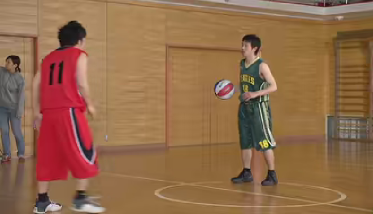
Figure 3: Selected frame from ‘BasketballPass’ test video coded by means of (a) the Chen’s DCT algorithm (PSNR 37.62 dB), (b) the modified RDCT (PSNR 37.42 dB), and (c) the proposed pruned approximation, with 76.2% less arithmetic operations then Chen’s DCT (PSNR 37.41 dB).

We considered real time video coding by embedding the proposed algorithms into the HEVC reference software by the Fraunhofer Heinrich Hertz Institute [42]. The original transform included in the HEVC reference software is a scaled approximation of Chen’s DCT algorithm. Our methodology consists of replacing the 8$\times$8 DCT algorithm of the reference software by the modified RDCT and the proposed pruned approximation.

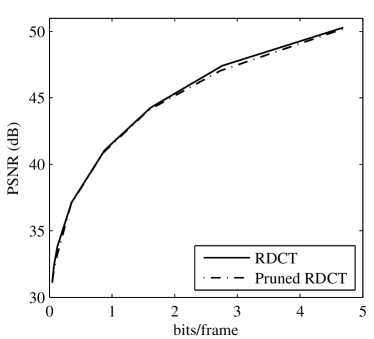
(a) PSNR values related to bit rate

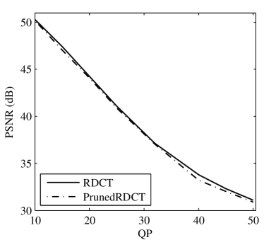
(b) PSNR values related to QP

Figure 4: RD curves for ‘BasketballPass’ test sequence.

Fig. 3 shows three 416$\times$240 frames of the ‘BasketballPass’ test sequence [52] obtained from the HEVC simulation. Resulting frames were coded using the Chen’s DCT algorithm (Fig. 3(a)), the modified RDCT (Fig. 3(b)), and the proposed pruned approximation (Fig. 3(c)). The PSNR values for these three frames are shown in Fig. 3. The pruned approximation effected minimal image degradation—less than 0.25 dB. On the other hand, computational complexity of the 8-point DCT was significantly reduced—76.2% less arithmetic operations when compared with the original Chen’s DCT algorithm.

We have also computed rate distortion (RD) curves for both RDCT and the proposed pruned approximation using standard video sequences [52]. For such, we varied the quantization point (QP) from 0 to 50 and computed the PSNR of the proposed pruned approximate with reference to the RDCT along with the bits/frame of the encoded video. As a result, we obtained the curves shown in Fig. 4(a). The PSNR values related to QP are shown in Figure 4(b). The difference in the rate points between the RDCT and the proposed pruned approximation is less than 0.57dB, which is smaller than $1.3~{}\%$.

6 Conclusion

In this paper, we presented a very low-complexity DCT approximation obtained via pruning. The resulting approximate transform requires only 10 additions and possesses performance metrics comparable with state-of-the-art methods, including the recent architecture presented in [40]. The proposed pruning approach can be adapted to other transformation methods, regardless of the transform size. By means of computational simulation, VLSI hardware realizations, and a full HEVC implementation, we demonstrated the practical relevance of our method as an image and video codec. Our goal with the image and video simulations is not to suggest the modification of existing standards, which would be unfeasible. Instead we aim at showing that (i) pruned approximations can be considered in tailored low-complexity, low-power systems for accelerated decoding of JPEG and HEVC and (ii) approximation methods combined with pruning are a viable alternative to the design of future standards.

For future work, we intend to apply the pruned approach to other discrete transforms methods for different blocklengths. In particular, the 4-, 16-, and 32-point DCT-based approximations are naturally fitted to the proposed approach. Moreover, a prospective study on the energy distribution in the transform domain could indicate the optimal number of coefficients to retain in the pruning process. Forthcoming applications include low-power wireless vision sensor networks and accelerated image decoding.

References

- [1] K. R. Rao and P. Yip, Discrete Cosine Transform: Algorithms, Advantages, Applications. San Diego, CA: Academic Press, 1990.
- [2] G. K. Wallace, “The JPEG still picture compression standard,” IEEE Transactions on Consumer Electronics, vol. 38, pp. xviii–xxxiv, 1992.
- [3] N. Roma and L. Sousa, “Efficient hybrid DCT-domain algorithm for video spatial downscaling,” EURASIP Journal on Advances in Signal Processing, vol. 2007, pp. 30–30, 2007.
- [4] International Organisation for Standardisation, “Generic coding of moving pictures and associated audio information – Part 2: Video,” ISO, ISO/IEC JTC1/SC29/WG11 - Coding of Moving Pictures and Audio, 1994.
- [5] International Telecommunication Union, “ITU-T recommendation H.261 version 1: Video codec for audiovisual services at kbits,” ITU-T, Tech. Rep., 1990.
- [6] ——, “ITU-T recommendation H.263 version 1: Video coding for low bit rate communication,” ITU-T, Tech. Rep., 1995.
- [7] T. Wiegand, G. J. Sullivan, G. Bjontegaard, and A. Luthra, “Overview of the H.264/AVC video coding standard,” IEEE Transactions on Circuits and Systems for Video Technology, vol. 13, pp. 560–576, 2003.
- [8] J. V. Team, “Recommendation H.264 and ISO/IEC 14 496–10 AVC: Draft ITU-T recommendation and final draft international standard of joint video specification,” ITU-T, Tech. Rep., 2003.
- [9] International Telecommunication Union, “High efficiency video coding: Recommendation ITU-T H.265,” ITU-T Series H: Audiovisual and Multimedia Systems, Tech. Rep., 2013.
- [10] M. T. Pourazad, C. Doutre, M. Azimi, and P. Nasiopoulos, “HEVC: The new gold standard for video compression: How does HEVC compare with H.264/AVC?” IEEE Consumer Electronics Magazine, vol. 1, pp. 36–46, Jul. 2012.
- [11] G. J. Sullivan, J. Ohm, W. Han, and T. Wiegand, “Overview of the high efficiency video coding (HEVC) standard,” IEEE Transactions on Circuits and Systems for Video Technology, vol. 22, pp. 1649–1668, Dec. 2012.
- [12] F. M. Bayer, R. J. Cintra, A. Madanayake, and U. S. Potluri, “Multiplierless approximate 4-point DCT VLSI architectures for transform block coding,” Electronics Letters, vol. 49, pp. 1532–1534, 2013.
- [13] J. Park, W. Nam, S. Han, and S. Lee, “2-D large inverse transform (1616, 3232) for HEVC (High Efficiency Video Coding),” Journal of Semiconductor Technology and Science, vol. 2, pp. 203–211, 2012.
- [14] S. Park and P. K. Meher, “Flexible integer DCT architectures for HEVC,” in IEEE International Symposium on Circuits and Systems (ISCAS), 2013, pp. 1376–1379.
- [15] U. S. Potluri, A. Madanayake, R. J. Cintra, F. M. Bayer, S. Kulasekera, and A. Edirisuriya, “Improved 8-point approximate DCT for image and video compression requiring only 14 additions,” IEEE Transactions on Circuits and Systems I: Regular Papers, vol. 61, no. 6, pp. 1727–1740, 2014.
- [16] J. Ohm, G. J. Sullivan, H. Schwarz, T. K. Tan, and T. Wiegand, “Comparison of the coding efficiency of video coding standards - including High Efficiency Video Coding (HEVC),” IEEE Transactions on Circuits and Systems for Video Technology, vol. 22, pp. 1669–1684, Dec. 2012.
- [17] T. I. Haweel, “A new square wave transform based on the DCT,” Signal Processing, vol. 82, pp. 2309–2319, 2001.
- [18] S. Bouguezel, M. O. Ahmad, and M. N. S. Swamy, “Low-complexity 88 transform for image compression,” Electronics Letters, vol. 44, pp. 1249–1250, Sep. 2008.
- [19] ——, “A fast 88 transform for image compression,” in International Conference on Microelectronics (ICM), Dec. 2009, pp. 74–77.
- [20] ——, “Binary discrete cosine and Hartley transforms,” IEEE Transactions on Circuits and Systems I: Regular Papers, vol. 60, pp. 989–1002, 2013.
- [21] R. J. Cintra and F. M. Bayer, “A DCT approximation for image compression,” IEEE Signal Processing Letters, vol. 18, pp. 579–582, Oct. 2011.
- [22] F. M. Bayer and R. J. Cintra, “DCT-like transform for image compression requires 14 additions only,” Electronics Letters, vol. 48, pp. 919–921, 2012.
- [23] R. J. Cintra, F. M. Bayer, and C. J. Tablada, “Low-complexity 8-point DCT approximations based on integer functions,” Signal Processing, vol. 99, pp. 201–214, 2014.
- [24] C. J. Tablada, F. M. Bayer, and R. J. Cintra, “A class of DCT approximations based on the Feig-Winograd algorithm,” Signal Processing, vol. 113, pp. 38–51, 2015. [Online]. Available: http://www.sciencedirect.com/science/article/pii/S0165168415000341
- [25] K. R. Rao and P. Yip, The Transform and Data Compression Handbook. CRC Press LLC, 2001.
- [26] Y. Huang, J. Wu, and C. Chang, “A generalized output pruning algorithm for matrix-vector multiplication and its application to compute pruning discrete cosine transform,” IEEE Transactions on Signal Processing, vol. 48, pp. 561–563, 2000.
- [27] J. Markel, “FFT pruning,” IEEE Transactions on Audio and Electroacoustics, vol. 19, pp. 305–311, 1971.
- [28] D. P. Skinner, “Pruning the decimation in-time FFT algorithm,” IEEE Transactions on Acoustics, Speech and Signal Processing, vol. 24, pp. 193–194, 1976.
- [29] R. G. Alves, P. L. Osorio, and M. N. S. Swamy, “General FFT pruning algorithm,” in 43rd IEEE Midwest Symposium on Circuits and Systems, vol. 3, 2000, pp. 1192–1195.
- [30] L. Wang, X. Zhou, G. E. Sobelman, and R. Liu, “Generic mixed-radix FFT pruning,” IEEE Signal Processing Letters, vol. 19, pp. 167–170, Mar. 2012.
- [31] R. Airoldi, O. Anjum, F. Garzia, A. M. Wyglinski, and J. Nurmi, “Energy-efficient fast Fourier transforms for cognitive radio systems,” IEEE Micro, vol. 30, pp. 66–76, Nov. 2010.
- [32] P. N. Whatmough, M. R. Perrett, S. Isam, and I. Darwazeh, “VLSI architecture for a reconfigurable spectrally efficient FDM baseband transmitter,” IEEE Transactions on Circuits and Systems I: Regular Papers, vol. 59, pp. 1107–1118, May 2012.
- [33] A. Oppenheim and R. Schafer, Discrete-Time Signal Processing, 3rd ed. Pearson, 2010.
- [34] J. H. Kim, J. G. Kim, Y. Ji, Y. Jung, and C. Won, “An islanding detection method for a grid-connected system based on the Goertzel algorithm,” IEEE Transactions on Power Electronics, vol. 26, pp. 1049–1055, Apr. 2011.
- [35] I. Carugati, S. Maestri, P. G. Donato, D. Carrica, and M. Benedetti, “Variable sampling period filter PLL for distorted three-phase systems,” IEEE Transactions on Power Electronics, vol. 27, pp. 321–330, Jan. 2012.
- [36] Z. Wang, “Pruning the fast discrete cosine transform,” IEEE Transactions on Communications, vol. 39, pp. 640–643, May 1991.
- [37] A. N. Skodras, “Fast discrete cosine transform pruning,” IEEE Transactions on Signal Processing, vol. 42, pp. 1833–1837, Jul. 1994.
- [38] V. Lecuire, L. Makkaoui, and J.-M. Moureaux, “Fast zonal DCT for energy conservation in wireless image sensor networks,” Electronics Letters, vol. 48, pp. 125–127, 2012.
- [39] G. Karakonstantis, N. Banerjee, and K. Roy, “Process-variation resilient and voltage-scalable DCT architecture for robust low-power computing,” IEEE Transactions on Very Large Scale Integration (VLSI) Systems, vol. 18, pp. 1461–1470, 2009.
- [40] N. Kouadria, N. Doghmane, D. Messadeg, and S. Harize, “Low complexity DCT for image compression in wireless visual sensor networks,” Electronics Letters, vol. 49, pp. 1531–1532, 2013.
- [41] P. K. Meher, S. Y. Park, B. K. Mohanty, K. S. Lim, and C. Yeo, “Efficient integer DCT architectures for HEVC,” IEEE Transactions on Circuits and Systems for Video Technology, vol. 24, pp. 168–178, Jan. 2014.
- [42] Joint Collaborative Team on Video Coding (JCT-VC), “HEVC reference software documentation,” Fraunhofer Heinrich Hertz Institute, Tech. Rep., 2013.
- [43] V. Britanak, P. Yip, and K. R. Rao, Discrete Cosine and Sine Transforms: General Properties, Fast Algorithms and Integer Approximation. Elsevier, 2007.
- [44] R. J. Cintra, “An integer approximation method for discrete sinusoidal transforms,” Journal of Circuits, Systems, and Signal Processing, vol. 30, pp. 1481–1501, 2011. [Online]. Available: http://www.springerlink.com/content/nw5u0267254t3683/
- [45] “The USC-SIPI image database,” http://sipi.usc.edu/database/, 2011, University of Southern California, Signal and Image Processing Institute.
- [46] R. E. Blahut, Fast Algorithms for Signal Processing. Cambridge University Press, 2010.
- [47] L. Makkaoui, V. Lecuire, and J. Moureaux, “Fast zonal DCT-based image compression for wireless camera sensor networks,” 2nd International Conference on Image Processing Theory Tools and Applications (IPTA), pp. 126–129, 2010.
- [48] G. A. F. Seber, A Matrix Handbook for Statisticians. John Wiley & Sons, Inc, 2008.
- [49] W. H. Chen, C. Smith, and S. Fralick, “A fast computational algorithm for the Discrete Cosine Transform,” IEEE Transactions on Communications, vol. 25, no. 9, pp. 1004–1009, Sep. 1977.
- [50] V. Bhaskaran and K. Konstantinides, Image and Video Compression Standards. Boston: Kluwer Academic Publishers, 1997.
- [51] Z. Wang, A. C. Bovik, H. R. Sheikh, and E. P. Simoncelli, “Image quality assessment: from error visibility to structural similarity,” IEEE Transactions on Image Processing, vol. 13, pp. 600–612, Apr. 2004.
- [52] “HEVC Test Video Sequence,” ftp://hvc:US88Hula@ftp.tnt.uni-hannover.de/testsequences, 2013, heinrich Hertz Institute.