POD/DEIM Reduced-Order Strategies for Efficient Four Dimensional Variational Data Assimilation

Abstract

This work studies reduced order modeling (ROM) approaches to speed up the solution of variational data assimilation problems with large scale nonlinear dynamical models. It is shown that a key requirement for a successful reduced order solution is that reduced order Karush-Kuhn-Tucker conditions accurately represent their full order counterparts. In particular, accurate reduced order approximations are needed for the forward and adjoint dynamical models, as well as for the reduced gradient. New strategies to construct reduced order based are developed for Proper Orthogonal Decomposition (POD) ROM data assimilation using both Galerkin and Petrov-Galerkin projections. For the first time POD, tensorial POD, and discrete empirical interpolation method (DEIM) are employed to develop reduced data assimilation systems for a geophysical flow model, namely, the two dimensional shallow water equations. Numerical experiments confirm the theoretical framework for Galerkin projection. In the case of Petrov-Galerkin projection, stabilization strategies must be considered for the reduced order models. The new reduced order shallow water data assimilation system provides analyses similar to those produced by the full resolution data assimilation system in one tenth of the computational time.

Keywords:  inverse problems; proper orthogonal decomposition; discrete empirical interpolation method (DEIM); reduced-order models (ROMs); shallow water equations; finite difference methods;

1 Introduction

Optimal control problems for nonlinear partial differential equations often require very large computational resources. Recently the reduced order approach applied to optimal control problems for partial differential equations has received increasing attention as a way of reducing the computational effort. The main idea is to project the dynamical system onto subspaces consisting of basis elements that represent the characteristics of the expected solution. These low order models serve as surrogates for the dynamical system in the optimization process and the resulting small optimization problems can be solved efficiently.

Application of Proper Orthogonal Decomposition (POD) to solve optimal control problems has proved to be successful as evidenced in the works of Kunisch and Volkwein [64], Kunisch et al. [68], Ito and Kunisch [56, 57], Kunisch and Xie [67]. However this approach may suffer from the fact that the basis elements are computed from a reference trajectory containing features which are quite different from those of the optimally controlled trajectory. A priori it is not evident what is the optimal strategy to generate snapshots for the reduced POD control procedure. A successful POD based reduced optimization should represent correctly the dynamics of the flow that is altered by the controller. To overcome the problem of unmodelled dynamics in the basis Afanasiev and Hinze [2], Ravindran [84], Kunisch and Volkwein [65], Bergmann et al. [19], Ravindran [83], Yue and Meerbergen [99], Zahr and Farhat [100], Zahr et al. [101] proposed to update the basis according to the current optimal control. In Arian et al. [9], Bergmann and Cordier [18], this updating technique was combined with a trust region (TR) strategy to determine whether after an optimization step an update of the POD-basis should be performed. Additional work on TR/POD proved its efficiency, see Bergmann and Cordier [17], Leibfritz and Volkwein [71], Sachs and Volkwein [89]. Other studies proposed to include time derivatives, nonlinear terms, and adjoint information (see Diwoky and Volkwein [40], Hinze and Volkwein [52], Hinze [51], Gubisch and Volkwein [48], Hay et al. [50], Carlberg and Farhat [24], Zahr and Farhat [100]) into POD basis for reduced order optimization purposes. A-posteriori analysis for POD applied to optimal control problems governed by parabolic and elliptic PDEs were developed in Hinze and Volkwein [52, 53], Tonna et al. [93], Tröltzsch and Volkwein [94], Kahlbacher and Volkwein [58], Kammann et al. [59]. Optimal snapshot location strategies for selecting additional snapshots at different time instances and for changing snapshots weights to represent more accurately the reduced order solutions were introduced in Kunisch and Volkwein [66]. Extension to parameterized nonlinear systems is available in Lass and Volkwein [69].

POD was successfully applied to solve strong constraint four dimensional variational (4D-Var) data assimilation problems for oceanic problems (Cao et al. [23], Fang et al. [43]) and atmospheric models (Chen et al. [30, 29], Daescu and Navon [36, 37], Du et al. [41]). A strategy that formulates first order optimality conditions starting from POD models has been implemented in 4D-Var systems in Vermeulen and Heemink [95], Sava [90], while hybrid methods using reduced adjoint models but optimizing in full space were introduced in Altaf et al. [5] and Ambrozic [6]. POD/DEIM has been employed to reduce the CPU complexity of a 1D Burgers 4D-Var system in Baumann [15]. Recently Amsallem et al. [8] used a two-step gappy POD procedure to decrease the computational complexity of the reduced nonlinear terms in the solution of shape optimization problems. Reduced basis approximation [13, 47, 78, 86, 38] is known to be very efficient for parameterized problems and has recently been applied in the context of reduced order optimization [48, 70, 74, 85].

This paper develops a systematic approach to POD bases selection for Petrov-Galerkin and Galerkin based reduced order data assimilation systems with non-linear models. The fundamental idea is to provide an order reduction strategy that ensures that the reduced Karush Kuhn Tucker (KKT) optimality conditions accurately approximate the full KKT optimality conditions [61, 63]. This property is guaranteed by constraining the reduced KKT conditions to coincide with the projected high-fidelity KKT equations. An error estimation result shows that smaller reduced order projection errors lead to more accurate reduced order optimal solutions. This result provides practical guidance for the construction of reduced order data assimilation systems, and for solving general reduced optimization problems. The research extends the results of Hinze and Volkwein [53] by considering nonlinear models and Petrov-Galerkin projections.

The proposed reduced order strategy is applied to solve a 4D-Var data assimilation problem with the two dimensional shallow water equations model. We compare three reduced 4D-Var data assimilation systems using three different POD Galerkin based reduced order methods namely standard POD, tensorial POD and standard POD/DEIM (see Ştefănescu et al. [35]). For Petrov-Galerkin projection stabilization strategies have to be considered. To the best of our knowledge this is the first application of POD/DEIM to obtain suboptimal solutions of reduced data assimilation system governed by a geophysical 2D flow model. For the mesh size used in our experiments the hybrid POD/DEIM reduced data assimilation system is approximately ten times faster then the full space data assimilation system, and this ratio is found out to be directly proportional with the mesh size.

The remainder of the paper is organized as follows. Section 2 introduces the optimality condition for the standard 4D-Var data assimilation problem. Section 3 reviews the reduced order modeling methodologies deployed in this work: standard, tensorial, and DEIM POD. Section 4 derives efficient POD bases selection strategies for reduced POD 4D-Var data assimilation systems governed by nonlinear state models using both Petrov-Galerkin and Galerkin projections. An estimation error result is also derived. Section 5 discusses the swallow water equations model and the three reduced order 4D-Var data assimilation systems employed for comparisons in this study. Results of extensive numerical experiments are discussed in Section 6 while conclusions are drawn in Section 7. Finally an appendix describing the high-fidelity alternating direction fully implicit (ADI) forward, tangent linear and adjoint shallow water equations (SWE) discrete models and reduced order SWE tensors is presented.

2 Strong constraint 4D-Var data assimilation system

Variational data assimilation seeks the optimal parameter values that provide the best fit (in some well defined sense) of model outputs with physical observations. In this presentation we focus on the traditional approach where the model parameters are the initial conditions ${\bf x}_{0}$, however the discussion can be easily generalized to further include other model parameter as control variables. In 4D-Var the objective function $\mathcal{J}:\mathbb{R}^{N_{\textnormal{state}}}\to\mathbb{R}$ that quantifies the model-data misfit and accounts for prior information is minimized:

$$\mathcal{J}({\mathbf{x}}_{0})=\frac{1}{2}\big{(}{\mathbf{x}}^{\rm b}_{0}-{\mathbf{x}}_{0}\big{)}^{T}{\mathbf{B}}_{0}^{-1}\big{(}{\mathbf{x}}^{\rm b}_{0}-{\mathbf{x}}_{0}\big{)}+\frac{1}{2}\sum_{i=0}^{N}\big{(}{\mathbf{y}}_{i}-\mathcal{H}_{i}\left({\mathbf{x}}_{i}\right)\big{)}^{T}\mathbf{R}_{i}^{-1}\big{(}{\mathbf{y}}_{i}-\mathcal{H}\left({\mathbf{x}}_{i}\right)\big{)},$$ (1a)

subject to the constraints posed by the nonlinear forward model dynamics

$${\mathbf{x}}_{i+1}=\mathcal{M}_{i,i+1}\left({\mathbf{x}}_{i}\right),\quad i=0,..,N-1.$$ (1b)

Here ${\mathbf{x}}^{\rm b}_{0}\in\mathbb{R}^{N_{\textnormal{state}}}$ is the background state and represents the best estimate of the true state ${\mathbf{x}}^{\rm true}_{0}\in\mathbb{R}^{N_{\textnormal{state}}}$ prior to any measurement being available, where $N_{\textnormal{state}}$ is the number of spatial discrete variables. The background errors are generally assumed to have a Gaussian distribution, i.e. ${\mathbf{x}}^{\rm b}_{0}-{\mathbf{x}}^{\rm true}_{0}\in\mathcal{N}(0,{\bf B}_{0})$, where ${\bf B}_{0}\in\mathbb{R}^{N_{\textnormal{state}}\times N_{\textnormal{state}}}$ is the background error covariance matrix. The nonlinear model $\mathcal{M}_{i,i+1}:\mathbb{R}^{N_{\textnormal{state}}}\to\mathbb{R}^{N_{\textnormal{state}}}$, $i=0,..,N-1$ advances the state vector in time from $t_{i}$ to $t_{i+1}$. The state variables are ${\mathbf{x}}_{i}\in\mathbb{R}^{N_{\textnormal{state}}}$ and the data (observation) values are ${\mathbf{y}}_{i}\in\mathbb{R}^{N_{\textnormal{obs}}}$ at times $t_{i}$, $i=0,..,N$. These observations are corrupted by instruments and representativeness errors [31] which are assumed to have a normal distribution $\mathcal{N}(0,{\mathbf{R}}_{i})$, where $\mathbf{R}_{i}\in\mathbb{R}^{N_{\textnormal{obs}}\times N_{\textnormal{obs}}}$ describes the observation error covariance matrix at time $t_{i}$. The nonlinear observation operator $\mathcal{H}_{i}:\mathbb{R}^{N_{\textnormal{state}}}\to\mathbb{R}^{N_{\textnormal{obs}}}$ maps the model state space to the observation space.

Using the Lagrange multiplier technique the constrained optimization problem (1) is replaced with the unconstrained optimization of the following Lagrangian function, $\mathcal{L}:\mathbb{R}^{N_{\textnormal{state}}}\to\mathbb{R}$

$$\begin{split}&\mathcal{L}({\mathbf{x}}_{0})=\frac{1}{2}\big{(}{\mathbf{x}}^{\rm b}_{0}-{\mathbf{x}}_{0}\big{)}^{T}{\mathbf{B}}_{0}^{-1}\big{(}{\mathbf{x}}^{\rm b}_{0}-{\mathbf{x}}_{0}\big{)}+\frac{1}{2}\sum_{i=0}^{N}\big{(}{\mathbf{y}}_{i}-\mathcal{H}({\bf x}_{i})\big{)}^{T}\mathbf{R}_{i}^{-1}\big{(}{\mathbf{y}}_{i}-\mathcal{H}({\bf x}_{i})\big{)}+\\ &\quad\quad\quad\quad\quad\quad\sum_{i=0}^{N-1}{\mathbf{\lambda}}_{i+1}^{T}\big{(}{\mathbf{x}}_{i+1}-\mathcal{M}_{i,i+1}\left({\mathbf{x}}_{i}\right)\big{)},\end{split}$$ (2)

where ${\mathbf{\lambda}}_{i}\in\mathbb{R}^{N_{\textnormal{state}}}$ is the Lagrange multipliers vector at observation time $t_{i}$.

Next we derive the first order optimality conditions. An infinitesimal change in $\mathcal{L}$ due to an infinitesimal change $\delta{\mathbf{x}}_{0}$ in ${\mathbf{x}}_{0}$ is

$$\begin{split}\delta\mathcal{L}({\mathbf{x}}_{0})&=-\delta{\mathbf{x}}_{0}^{T}{\mathbf{B}}_{0}^{-1}\big{(}{\mathbf{x}}^{\rm b}_{0}-{\mathbf{x}}_{0}\big{)}-\sum_{i=0}^{N}\delta{\mathbf{x}}_{i}^{T}{\mathbf{H}}_{i}^{T}\mathbf{R}_{i}^{-1}\big{(}{\mathbf{y}}_{i}-\mathcal{H}({\mathbf{x}}_{i})\big{)}+\\ &\sum_{i=0}^{N-1}\lambda_{i+1}^{T}\big{(}\delta{\mathbf{x}}_{i+1}-{\mathbf{M}}_{i,i+1}\delta{\mathbf{x}}_{i}\big{)}+\sum_{i=0}^{N-1}\delta{\mathbf{\lambda}}_{i+1}^{T}\big{(}{\mathbf{x}}_{i+1}-\mathcal{M}_{i,i+1}\left({\mathbf{x}}_{i}\right)\big{)},\\ \end{split}$$ (3)

where $\delta{\mathbf{x}}_{i}=(\partial{\mathbf{x}}_{i}/\partial{\mathbf{x}}_{0})\,\delta{\mathbf{x}}_{0}$, and ${\bf H}_{i}$ and ${\mathbf{M}}_{i,i+1}$ are the Jacobian matrices of $\mathcal{H}_{i},~{}i=0,..,N$ and $\mathcal{M}_{i,i+1}$ for all time instances $t_{i}$, $i=0,\dots,N-1$, at ${\bf x}_{i}$,

$${\bf H}_{i}=\frac{\partial\mathcal{H}_{i}}{\partial{\mathbf{x}}_{i}}({\mathbf{x}}_{i})\in\mathbb{R}^{N_{\textnormal{obs}}\times N_{\textnormal{state}}},\quad{\mathbf{M}}_{i,i+1}=\frac{\partial\mathcal{M}_{i,i+1}}{\partial{\mathbf{x}}_{i}}({\mathbf{x}}_{i})\in\mathbb{R}^{N_{\textnormal{state}}\times N_{\textnormal{state}}}.$$

The corresponding adjoint operators are ${\bf H}_{i}^{T}\in\mathbb{R}^{N_{\textnormal{state}}\times N_{\textnormal{obs}}}$ and ${\bf M}_{i+1,i}^{*}\in\mathbb{R}^{N_{\textnormal{state}}\times N_{\textnormal{state}}}$, respectively, and satisfy

$$\begin{split}\langle{\bf H}_{i}z_{1},y_{1}\rangle_{\mathbb{R}^{N_{\textnormal{obs}}}}=\langle z_{1},{\bf H}^{T}_{i}y_{1}\rangle_{\mathbb{R}^{N_{\textnormal{state}}}},~{}\forall z_{1}\in{\mathbb{R}^{N_{\textnormal{state}}}},~{}\forall y_{1}\in{\mathbb{R}^{N_{\textnormal{obs}}}},\\ \langle{\mathbf{M}}_{i,i+1}z_{1},z_{2}\rangle_{\mathbb{R}^{N_{\textnormal{state}}}}=\langle z_{1},{\mathbf{M}}^{*}_{i+1,i}z_{2}\rangle_{\mathbb{R}^{N_{\textnormal{state}}}},\quad\forall z_{1},~{}z_{2}\in\mathcal{\mathbb{R}^{N_{\textnormal{state}}}},\\ \end{split}$$

where $\langle\cdot,\cdot\rangle_{\mathbb{R}^{N_{\textnormal{state}}}},~{}\langle\cdot,\cdot\rangle_{\mathbb{R}^{N_{\textnormal{obs}}}}$ are the corresponding Euclidian products. The adjoint operators of ${\bf H}_{i}$ and ${\mathbf{M}}_{i,i+1}$ are their transposes. We prefer to use the notation ${\bf M}_{i+1,i}^{*}={\bf M}_{i,i+1}^{T}$ to show that the corresponding adjoint model runs backwards in time. After rearranging (3) and using the definition of adjoint operators one obtains:

$$\delta\mathcal{L}({\mathbf{x}}_{0}) = -\delta{\mathbf{x}}_{0}^{T}{\mathbf{B}}_{0}^{-1}\big{(}{\mathbf{x}}^{\rm b}_{0}-{\bf x}_{0}\big{)}+\sum_{i=1}^{N-1}\delta{\mathbf{x}}_{i}^{T}\Bigl{(}{\mathbf{\lambda}}_{i}-{\mathbf{M}}_{i+1,i}^{*}\mathbf{\lambda}_{i+1}-{\bf H}_{i}^{T}\mathbf{R}_{i}^{-1}\big{(}{\mathbf{y}}_{i}-\mathcal{H}({\mathbf{x}}_{i})\Bigr{)}$$

$$+\delta{\mathbf{x}}_{N}^{T}\Bigl{(}{\mathbf{\lambda}}_{N}-{\bf H}_{N}^{T}\mathbf{R}_{N}^{-1}\big{(}{\mathbf{y}}_{N}-\mathcal{H}({\mathbf{x}}_{N})\big{)}\Bigr{)}-\delta{\mathbf{x}}_{0}^{T}\Bigl{(}{\bf H}_{0}^{T}\mathbf{R}_{0}^{-1}\big{(}{\mathbf{y}}_{0}-\mathcal{H}({\mathbf{x}}_{0})\big{)}+{\mathbf{M}}_{1,0}^{*}\mathbf{\lambda}_{1}\Bigr{)}$$

$$+\sum_{i=0}^{N-1}\delta{\mathbf{\lambda}}_{i+1}^{T}\big{(}{\mathbf{x}}_{i+1}-\mathcal{M}_{i,i+1}\left({\mathbf{x}}_{i}\right)\big{)}.$$

The first order necessary optimality conditions for the Full order 4D-Var are obtained by zeroing the variations of (2):

Full order forward model: (5a)

$$\qquad{\mathbf{x}}_{i+1}=\mathcal{M}_{i,i+1}\left({\mathbf{x}}_{i}\right),\quad i=0,..,N-1;$$

Full order adjoint model: (5b)

$$\qquad\mathbf{\lambda}_{N}={\mathbf{H}}_{N}^{T}\mathbf{R}_{N}^{-1}\big{(}{\bf y}_{N}-\mathcal{H}({\mathbf{x}}_{N})\big{)},$$

$$\qquad{\mathbf{\lambda}}_{i}={\mathbf{M}}_{i+1,i}^{*}\mathbf{\lambda}_{i+1}+{\mathbf{H}}_{i}^{T}\mathbf{R}_{i}^{-1}\big{(}{\bf y}_{i}-\mathcal{H}({\mathbf{x}}_{i})\big{)},\quad i=N-1,..,0;$$

Full order gradient of the cost function: (5c)

$$\qquad\nabla_{{\bf x}_{0}}\mathcal{L}=-{\mathbf{B}}_{0}^{-1}\big{(}{\mathbf{x}}^{\rm b}_{0}-{\mathbf{x}}_{0}\big{)}-{\mathbf{\lambda}}_{0}=0.$$

3 Reduced order forward modeling

The most prevalent basis selection method for model reduction of nonlinear problems is the proper orthogonal decomposition, also known as Karhunen-Loève expansion [60, 72], principal component analysis [55], and empirical orthogonal functions [73].

Three reduced order models will be considered in this paper: standard POD (SPOD), tensorial POD (TPOD), and standard POD/Discrete Empirical Interpolation Method (POD/DEIM), which were described in Ştefănescu et al. [35] and Ştefănescu and Navon [32]. The reduced Jacobians required by the ADI schemes are obtained analytically for all three ROMs via tensorial calculus and their computational complexity depends only on $k$, the dimension of POD basis. The above mentioned methods differ in the way the nonlinear terms are treated. We illustrate the application of the methods to reduce a polynomial quadratic nonlinearity $N(\mathbf{x}_{i})={\bf x}_{i}^{2},~{}i=0,..,N$, where vector powers are taken component-wise. Details regarding standard POD approach including the snapshot procedure, POD basis computation and the corresponding reduced equations can be found in [35]. We assume a Petrov-Galerkin projection for constructing the reduced order models with the two biorthogonal projection matrices $U,W\in\mathbb{R}^{N_{\textnormal{state}}\times k}$, $W^{T}U=I_{k}$, where $I_{k}$ is the identity matrix of order $k$, $k\ll N_{\textnormal{state}}$. $U$ denotes the POD basis (trial functions) and the test functions are stored in $W$. We assume a POD expansion of the state ${\mathbf{x}}\approx U{\tilde{\mathbf{x}}}$, and the reduced order quadratic term $\widetilde{N}({\bf\tilde{x}})\approx N(\mathbf{x})$ is detailed bellow. For simplicity we removed the index $i$ from the state variable notation, thus $\mathbf{x}\in\mathbb{R}^{N_{\textnormal{state}}},~{}{\tilde{\mathbf{x}}}\in\mathbb{R}^{k}$.

Standard POD

$$\widetilde{N}({\bf\tilde{x}})=\underbrace{W^{T}}_{k\times N_{\textnormal{state}}}\underbrace{\big{(}U{\bf\tilde{x}}\big{)}^{2}}_{N_{\textnormal{state}}\times 1},\quad\widetilde{N}({\bf\tilde{x}})\in\mathbb{R}^{k},$$ (6)

where vector powers are taken component-wise.

Tensorial POD

$$\widetilde{N}({\bf\tilde{x}})=\big{[}{\widetilde{N}}_{i}\big{]}_{i=1,..,k}\in\mathbb{R}^{k};\quad\widetilde{N}_{i}=\sum_{j=1}^{k}\sum_{l=1}^{k}T_{i,j,l}{\tilde{x}}_{j}{\tilde{x}}_{l},$$ (7)

where the rank-three tensor $T$ is defined as

$$T=\left(T_{i,j,l}\right)_{i,j,l=1,..,k}\in\mathbb{R}^{k\times k\times k},\quad T_{i,j,l}=\sum_{r=1}^{N_{\textnormal{state}}}W_{r,i}U_{r,j}U_{r,l}.$$

Standard POD/DEIM

$$\tilde{N}({\bf\tilde{x}})\approx\underbrace{W^{T}V(P^{T}V)^{-1}}_{k\times m}\underbrace{\left(P^{T}U{\bf\tilde{x}}\right)^{2}}_{m\times 1},$$ (8)

where $m$ is the number of interpolation points, $V\in\mathbb{R}^{N_{\textnormal{state}}\times m}$ gathers the first $m$ POD basis modes of the nonlinear term while $P\in\mathbb{R}^{{N_{\textnormal{state}}}\times m}$ is the DEIM interpolation selection matrix (Chaturantabut [26], Chaturantabut and Sorensen [27, 28]).

The systematic application of these techniques in the Petrov-Galerkin projection framework to (1b) leads to the following reduced order forward model

$${\bf\tilde{x}}_{i+1}=\widetilde{\mathcal{M}}_{i,i+1}\left({\bf\tilde{x}}_{i}\right),\quad\widetilde{\mathcal{M}}_{i,i+1}\left({\bf\tilde{x}}_{i}\right)=W^{T}\mathcal{M}_{i,i+1}\left(U{\bf\tilde{x}}_{i}\right),\quad i=0,..,N-1.$$ (9)

4 Reduced order 4D-Var data assimilation

Two major strategies for solving data assimilation problems with reduced order models have been discussed in the literature. The “reduced adjoint” (RA) approach [5] projects the first order optimality equation (5b) of the full system onto some POD reduced space and solves the optimization problem in the full space, while the “adjoint of reduced” (AR) approach [80, 95] formulates the first order optimality conditions from the forward reduced order model (10b) and searches for the optimal solution by solving a collection of reduced optimization problems in the reduced space. Reduced order formulation of the cost function is employed in the “adjoint of reduced” case [39]. In the control literature these approaches are referred to as “design-then-reduce” and “reduce-then-design” methods [11, 12].

The “reduced of adjoint” approach avoids the implementation of the adjoint of the tangent linear approximation of the original nonlinear model by replacing it with a reduced adjoint. This is obtained by projecting the full set of equations onto a POD space build on the snapshots computed with the high-resolution forward model. Once the gradient is obtained in reduced space it is projected back in full space and the minimization process is carried in full space. The drawbacks of this technique consist in the use of an inaccurate low-order adjoint model with respect to its full counterpart that may lead to erroneous gradients. Moreover the computational cost of the optimization system is still high since it requires the run of the full forward model to evaluate the cost function during the minimization procedure.

A major concern with the “adjoint of reduced” approach is the lack of accuracy in the optimality conditions with respect to the full system. The reduced forward model is accurate, but its adjoint and optimality condition poorly approximate their full counterparts since the POD basis relies only on forward dynamics information. Consequently both the RA and the AR methods may lead to inaccurate suboptimal solutions.

Snapshots from both primal and dual systems have been used for balanced truncation of a linear state-system. [98]. Hinze and Volkwein [54] developed a-priori error estimates for linear quadratic optimal control problems using proper orthogonal decomposition. They state that error estimates for the adjoint state yield error estimates of the control suggesting that accurate reduced adjoint models with respect to the full adjoint model lead to more accurate suboptimal surrogate solutions. Numerical results confirmed that a POD manifold built on snapshots taken from both forward and adjoint trajectories provides more accurate reduced optimization systems.

This work develops a systematic approach to select POD bases for reduced order data assimilation with non-linear models. Accuracy of the reduced optimum is ensured by constraining the “adjoint of reduced” optimality conditions to coincide with a generalized “reduced of adjoint” KKT conditions obtained by projecting all equations (5) onto appropriate reduced manifolds. This leads to the concept of accurate reduced KKT conditions and provides practical guidance to construct reduced order manifolds for reduced order optimization. The new strategy, named ARRA, provides a unified framework where the AR and RA approaches lead to the same solution for general reduced order optimization problems. In the ARRA approach the model reduction and adjoint differentiation operations commute.

4.1 The “adjoint of reduced forward model” approach

We first define the objective function. To this end we assume that the forward POD manifold $\mathbf{U}_{\textnormal{f}}$ is computed using only snapshots of the full forward model solution (the subscript denotes that only forward dynamics information is used for POD basis construction). The Petrov-Galerkin (PG) test functions $\mathbf{W}_{\textnormal{f}}$ are different than the trial functions $\mathbf{U}_{\textnormal{f}}$. Assuming a POD expansion of ${\bf x}_{i}\approx\mathbf{U}_{\textnormal{f}}\,{\bf\tilde{x}}_{i},~{}i=0,..,N,$ the reduced data assimilation problem minimizes the following reduced order cost function $\mathcal{J}^{\textsc{pod}}:\mathbb{R}^{k}\to\mathbb{R}$

$$\begin{split}&\mathcal{J}^{\textsc{pod}}({\bf\tilde{x}}_{0})=\frac{1}{2}\big{(}{\mathbf{x}}^{\rm b}_{0}-\mathbf{U}_{\textnormal{f}}\,{\bf\tilde{x}}_{0}\big{)}^{T}{\bf B}_{0}^{-1}\big{(}{\mathbf{x}}^{\rm b}_{0}-\mathbf{U}_{\textnormal{f}}\tilde{\bf x}_{0}\big{)}\\ &\quad\quad\quad\quad\quad\quad+\frac{1}{2}\sum_{i=0}^{N}\big{(}{\mathbf{y}}_{i}-\mathcal{H}_{i}(\mathbf{U}_{\textnormal{f}}\,{\bf\tilde{x}}_{i})\big{)}^{T}\mathbf{R}_{i}^{-1}\big{(}{\mathbf{y}}_{i}-\mathcal{H}_{i}(\mathbf{U}_{\textnormal{f}}\,{\bf\tilde{x}}_{i})\big{)}^{T},\end{split}$$ (10a)

subject to the constraints posed by the reduced order model dynamics

$${\bf\tilde{x}}_{i+1}=\widetilde{\mathcal{M}}_{i,i+1}\left({\bf\tilde{x}}_{i}\right),\quad\widetilde{\mathcal{M}}_{i,i+1}\left({\bf\tilde{x}}_{i}\right)=\mathbf{W}_{\textnormal{f}}^{T}\mathcal{M}_{i,i+1}\left(\mathbf{U}_{\textnormal{f}}\,{\bf\tilde{x}}_{i}\right),\quad i=0,..,N-1.$$ (10b)

An observation operator that maps directly from the reduced model space to observations space may be introduced. For clarity sake we will continue to use operator notation $\mathcal{H}_{i},~{}i=0,..,N$ and $\widetilde{\mathcal{M}}_{i,i+1}$ denotes the PG reduced order forward model that propagates the reduced order state from $t_{i}$ to $t_{i+1}$ for $i=0,..,N-1$.

Next the constrained optimization problem (10) is replaced by an unconstrained one for the reduced Lagrangian function $\mathcal{L}^{\textsc{pod}}:\mathbb{R}^{k}\to\mathbb{R}$

$$\mathcal{L}^{\textsc{pod}}({\bf\tilde{x}}_{0}) = \frac{1}{2}\big{(}{\mathbf{x}}^{\rm b}_{0}-\mathbf{U}_{\textnormal{f}}\,{\bf\tilde{x}}_{0}\big{)}^{T}{\bf B}_{0}^{-1}\big{(}{\mathbf{x}}^{\rm b}_{0}-\mathbf{U}_{\textnormal{f}}\,{\bf\tilde{x}}_{0}\big{)}$$

$$+\frac{1}{2}\sum_{i=0}^{N}\big{(}{\mathbf{y}}_{i}-\mathcal{H}_{i}(\mathbf{U}_{\textnormal{f}}\,{\bf\tilde{x}}_{i})\big{)}^{T}\mathbf{R}_{i}^{-1}\big{(}{\mathbf{y}}_{i}-\mathcal{H}_{i}(\mathbf{U}_{\textnormal{f}}\,{\bf\tilde{x}}_{i})\big{)}$$

$$+\sum_{i=0}^{N-1}{\bf\tilde{\lambda}}_{i+1}^{T}\big{(}{\bf\tilde{x}}_{i+1}-\widetilde{\mathcal{M}}_{i,i+1}\left({\bf\tilde{x}}_{i}\right)\big{)},$$

where ${\bf\tilde{\lambda}}_{i}\in\mathbb{R}^{k}\in,~{}i=1,..,N$. The variation of $\mathcal{L}^{\textsc{pod}}$ is given by

$$\begin{split}&\delta\mathcal{L}^{\textsc{pod}}({\bf\tilde{x}}_{0})=-\delta{\bf\tilde{x}}_{0}^{T}{\mathbf{B}}_{0}^{-1}\big{(}{\mathbf{x}}^{\rm b}_{0}-\mathbf{U}_{\textnormal{f}}\,{\bf\tilde{x}}_{0}\big{)}+\sum_{i=1}^{N-1}\delta{\bf\tilde{x}}_{i}^{T}\Bigl{(}{\bf\tilde{\lambda}}_{i}-{\bf\widetilde{M}}_{i+1,i}^{*}{\bf\tilde{\lambda}}_{i+1}\\ &\quad\quad-\mathbf{U}_{\textnormal{f}}^{T}{\bf\widehat{H}}_{i}^{T}\mathbf{R}_{i}^{-1}\big{(}{\mathbf{y}}_{i}-\mathcal{H}_{i}(\mathbf{U}_{\textnormal{f}}\,{\bf\tilde{x}}_{i})\Bigr{)}+\delta{\bf\tilde{x}}_{N}^{T}\Bigl{(}{\bf\tilde{\lambda}}_{N}-\mathbf{U}_{\textnormal{f}}^{T}{\bf\widehat{H}}_{N}^{T}\mathbf{R}_{N}^{-1}\big{(}{\bf y}_{N}-\mathcal{H}_{i}(\mathbf{U}_{\textnormal{f}}\,{\bf\tilde{x}}_{N})\big{)}\Bigr{)}\\ &\quad\quad-\delta{\bf\tilde{x}}_{0}^{T}\Bigl{(}\mathbf{U}_{\textnormal{f}}^{T}{\bf H}_{0}^{T}\mathbf{R}_{0}^{-1}\big{(}{\mathbf{y}}_{0}-\mathcal{H}_{0}(\mathbf{U}_{\textnormal{f}}\,{\bf\tilde{x}}_{0})\big{)}+{\bf\widetilde{M}}_{1,0}^{*}{\bf\tilde{\lambda}}_{1}\Bigr{)}+\sum_{i=0}^{N-1}\delta{\bf\tilde{\lambda}}_{i+1}^{T}\big{(}{\bf\tilde{x}}_{i+1}-\widetilde{\mathcal{M}}_{i,i+1}\left({\bf\tilde{x}}_{i}\right)\big{)},\\ \end{split}$$ (12)

where

$${\bf\widetilde{M}}_{i+1,i}^{*}=\mathbf{U}_{\textnormal{f}}^{T}{\bf\widehat{M}}_{i+1,i}^{*}\mathbf{W}_{\textnormal{f}},\quad i=0,..,N-1$$

is the adjoint of the reduced order linearized forward model $\mathcal{M}_{i,i+1}$. The operators ${\bf\widehat{H}}_{i}^{T},~{}i=0,..,N$ and ${\bf\widehat{M}}_{i+1,i}^{*},~{}i=0,..,N-1$ are the high-fidelity adjoint models evaluated at $\mathbf{U}_{\textnormal{f}}\,{\bf\tilde{x}}_{i}$. The reduced KKT conditions are obtained by setting the variations of (12) to zero:

AR reduced forward model:

$$\qquad{\bf\tilde{x}}_{i+1}=\widetilde{\mathcal{M}}_{i,i+1}\left({\bf\tilde{x}}_{i}\right),\quad\widetilde{\mathcal{M}}_{i,i+1}\left({\bf\tilde{x}}_{i}\right)=\mathbf{W}_{\textnormal{f}}^{T}\,{\mathcal{M}}_{i,i+1}\left({\mathbf{U}_{\textnormal{f}}\,\bf\tilde{x}}_{i}\right),\quad i=0,..,N-1;$$

AR reduced adjoint model:

$$\qquad{\bf\tilde{\lambda}}_{N}=\mathbf{U}_{\textnormal{f}}^{T}\,{\bf\widehat{H}}_{N}^{T}\,\mathbf{R}_{N}^{-1}\,\big{(}{\bf y}_{N}-\mathcal{H}_{i}(\mathbf{U}_{\textnormal{f}}\,{\bf\tilde{x}}_{N})\big{)},\quad\quad\quad\quad\quad\quad\quad$$

$$\qquad{\bf\tilde{\lambda}}_{i}=\mathbf{U}_{\textnormal{f}}^{T}\,{\bf\widehat{M}}_{i+1,i}^{*}\,\mathbf{W}_{\textnormal{f}}\,{\bf\tilde{\lambda}}_{i+1}+\mathbf{U}_{\textnormal{f}}^{T}\,{\bf\widehat{H}}_{i}^{T}\,\mathbf{R}_{i}^{-1}\,\big{(}{\mathbf{y}}_{i}-\mathcal{H}_{i}(\mathbf{U}_{\textnormal{f}}\,{\bf\tilde{x}}_{i})\big{)},\quad i=N-1,..,0;$$

$$\textnormal{{\it AR cost function gradient} }:$$

$$\qquad\nabla_{{\bf\tilde{x}}_{0}}\mathcal{L}^{\textsc{pod}}=-\mathbf{U}_{\textnormal{f}}^{T}{\bf B}_{0}^{-1}\big{(}{\mathbf{x}}^{\rm b}_{0}-\mathbf{U}_{\textnormal{f}}\,{\bf\tilde{x}}_{0}\big{)}-{\bf\tilde{\lambda}}_{0}=0.$$

A comparison between the KKT systems of the reduced order optimization (13) and of the full order problem (5) reveals that the reduced forward model (13) is, by construction, an accurate approximation of the full forward model (5a). However, the AR adjoint (13) and AR gradient (13) equations are constructed using the forward model bases and test functions, and are not guaranteed to approximate well the corresponding full adjoint (5b) and full gradient (5c) equations, respectively.

4.2 The “reduced order adjoint model” approach

In a general RA framework the optimality conditions (5) are projected onto reduced order subspaces. The forward, adjoint, and gradient variables are reduced using forward, adjoint, and gradient bases $\mathbf{U}_{\textnormal{f}},~{}\mathbf{U}_{\textnormal{a}}$ and $\mathbf{U}_{\textnormal{g}}$ such that ${\mathbf{x}}_{i}\approx\mathbf{U}_{\textnormal{f}}\,{\bf\tilde{x}}_{i},~{}{\bm{\lambda}}_{i}\approx\mathbf{U}_{\textnormal{a}}\,{\bm{\tilde{}}\lambda}_{i},~{}i=0,..,N$, and $\nabla_{{\mathbf{x}}_{0}}\mathcal{L}\approx\mathbf{U}_{\textnormal{g}}\,\nabla_{{\bf\tilde{x}}_{0}}\mathcal{L}^{\textsc{pod}}$. The test functions for the forward, adjoint, and gradient equations are $\mathbf{W}_{\textnormal{f}}$, $\mathbf{W}_{\textnormal{a}}$, and $\mathbf{W}_{\textnormal{g}}$, respectively. The objective function to be minimized is (10a). The projected KKT conditions read:

RA reduced forward model: (14a)

$$\qquad{\bf\tilde{x}}_{i+1}=\widetilde{\mathcal{M}}_{i,i+1}\,\left({\bf\tilde{x}}_{i}\right),\quad i=0,..,N-1;$$

RA reduced adjoint model: (14b)

$$\qquad{\bf\tilde{\lambda}}_{N}=\mathbf{W}_{\textnormal{a}}^{T}\,{\bf H}_{N}^{T}\,\mathbf{R}_{N}^{-1}\,\big{(}{\bf y}_{N}-\mathcal{H}_{i}(\mathbf{U}_{\textnormal{f}}{{\bf\tilde{x}}}_{N})\big{)},$$

$$\qquad{\bf\tilde{\lambda}}_{i}=\mathbf{W}_{\textnormal{a}}^{T}\,{\bf M}_{i+1,i}^{*}\,\mathbf{U}_{\textnormal{a}}\,{\bf\tilde{\lambda}_{i+1}}+\mathbf{W}_{\textnormal{a}}^{T}\,{\bf H}_{i}^{T}\,\mathbf{R}_{i}^{-1}\,\big{(}{\bf y}_{i}-\mathcal{H}_{i}({\bf x}_{i})\big{)},\quad i=N-1,..,0;$$

RA cost function gradient: (14c)

$$\qquad\nabla_{{\bf\tilde{x}}_{0}}\mathcal{L}^{\textsc{pod}}=-\mathbf{W}_{\textnormal{g}}^{T}\,\big{[}{\mathbf{B}}_{0}^{-1}\,\big{(}{\mathbf{x}}^{\rm b}_{0}-\mathbf{U}_{\textnormal{f}}\,{\bf\tilde{x}}_{0}\big{)}-\mathbf{U}_{\textnormal{a}}\,{\bf\tilde{\lambda}_{0}}\big{]}=0.$$

With appropriately chosen basis and test functions the system (14) can accurately approximate the full order optimality conditions (5). However, in general the projected system (14) does not represent the KKT conditions of any optimization problem, and therefore the RA approach does not automatically provide a consistent optimization framework in the sense given by the following definition.

Definition 4.1

A reduced KKT system (14) is said to be consistent if it represents the first order optimality conditions of some reduced order optimization problem.

By constraining the projected KKT (14) to match the “adjoint of reduced” optimality conditions (13), one can obtain a consistent optimality framework where the reduced system accurately approximates the high-fidelity optimality system (5). This new theoretical framework is discussed next.

4.3 The ARRA approach: ensuring accuracy of the first order optimality system

The proposed method constructs the reduced order optimization problem (10) such that the reduced KKT equations (13) accurately approximate the high-fidelity KKT conditions (5).

1. In the AR approach the first KKT condition (13) is an accurate approximation of (5a) by construction, since $\mathbf{U}_{\textnormal{f}}$ is constructed with snapshots of the full forward trajectory, i.e. ${\bf x}\approx\mathbf{U}_{\textnormal{f}}\,{\bf\tilde{x}}$.

2. Next, we require that the AR reduced adjoint model (13) is a low-order accurate approximation of the full adjoint model (5b). This is achieved by imposing that the AR adjoint (13) is a reduced-order model obtained by projecting the full adjoint equation into a reduced basis containing high fidelity adjoint information, i.e., has the RA form (14b). We obtain

   $$\mathbf{W}_{\textnormal{f}}=\mathbf{U}_{\textnormal{a}}\textnormal{ and }\mathbf{W}_{\textnormal{a}}=\mathbf{U}_{\textnormal{f}}.$$ (15)

   The forward test functions are the bases $\mathbf{W}_{\textnormal{f}}=\mathbf{U}_{\textnormal{a}}$ constructed with snapshots of the full adjoint trajectory, i.e. ${\bf\lambda}\approx\mathbf{U}_{\textnormal{a}}\,{\bf\tilde{\lambda}}$. Note that in (14b) the model and observation operators are evaluated at the full forward solution ${\bf x}$ and then projected. In (13) the model and observation operators are evaluated at the reduced forward solution $\mathbf{U}_{\textnormal{f}}\,{\bf\tilde{x}}_{i}\approx{\bf x}_{i}$. The adjoint test functions are the bases $\mathbf{W}_{\textnormal{a}}=\mathbf{U}_{\textnormal{f}}$ constructed with snapshots of the full forward trajectory.

3. With (15) the reduced gradient equation (13) becomes

   $$\nabla_{{\bf\tilde{x}}_{0}}\mathcal{L}^{\textsc{pod}}=\mathbf{U}_{\textnormal{f}}^{T}\left(-{\bf B}_{0}^{-1}\big{(}{\mathbf{x}}^{\rm b}_{0}-\mathbf{U}_{\textnormal{f}}\,{\bf\tilde{x}}_{0}\big{)}-\mathbf{U}_{\textnormal{a}}{\bm{\tilde{}}\lambda}_{0}\right)=0.$$ (16)

   We require that the gradient (16) is a low-order accurate approximation of the full gradient (5c) obtained by projecting it, i.e., has the RA gradient form (14c). This leads to

   $$\mathbf{W}_{\textnormal{g}}=\mathbf{U}_{\textnormal{f}}.$$ (17)

   From PG construction, $\mathbf{U}_{\textnormal{g}}$ is orthogonal with $\mathbf{W}_{\textnormal{g}}=\mathbf{U}_{\textnormal{f}}$, thus a good choice for $\mathbf{U}_{\textnormal{g}}$ is $\mathbf{U}_{\textnormal{a}}$ where the gradient of the background term with respect to the initial conditions $-{\bf B}_{0}^{-1}\big{(}{\mathbf{x}}_{0}^{{\rm b}}-{\bf x}_{0}\big{)}$ is used to enrich the high-fidelity adjoint snapshots matrix, i.e. $\mathbf{U}_{\textnormal{g}}=\mathbf{U}_{\textnormal{a}}$.

We refer to the technique described above as “adjoint of reduced = reduced of adjoint” (ARRA) framework. The ARRA reduced order optimality system is:

ARRA reduced forward model: (18a)

$$\qquad{\bf\tilde{x}}_{i+1}=\widetilde{\mathcal{M}}_{i,i+1}\left({\bf\tilde{x}}_{i}\right),\quad\widetilde{\mathcal{M}}_{i,i+1}\left({\bf\tilde{x}}_{i}\right)=\mathbf{U}_{\textnormal{a}}^{T}\,{\mathcal{M}}_{i,i+1}\left({\mathbf{U}_{\textnormal{f}}\,\bf\tilde{x}}_{i}\right),\quad i=0,..,N-1,$$

ARRA reduced adjoint model: (18b)

$$\qquad{\bf\tilde{\lambda}}_{N}=\mathbf{U}_{\textnormal{f}}^{T}{\bf\widehat{H}}_{N}^{T}\mathbf{R}_{N}^{-1}\big{(}{\bf y}_{N}-\mathcal{H}(\mathbf{U}_{\textnormal{f}}\,{\bf\tilde{x}}_{N})\big{)},\quad\quad\quad\quad\quad\quad\quad$$

$$\qquad{\bf\tilde{\lambda}}_{i}=\mathbf{U}_{\textnormal{f}}^{T}{\bf\widehat{M}}_{i,i+1}^{T}\mathbf{U}_{\textnormal{a}}{\bf\tilde{\lambda}}_{i+1}+\mathbf{U}_{\textnormal{f}}^{T}{\bf\widehat{H}}_{i}^{T}\mathbf{R}_{i}^{-1}\big{(}{\mathbf{y}}_{i}-\mathcal{H}(\mathbf{U}_{\textnormal{f}}\,{\bf\tilde{x}}_{i})\big{)},\quad i=N-1,..,0,$$

$$\textnormal{{\it ARRA cost function gradient} }:$$ (18c)

$$\qquad\nabla_{{\bf\tilde{x}}_{0}}\mathcal{L}^{\textsc{pod}}=-\mathbf{U}_{\textnormal{f}}^{T}\,{\bf B}_{0}^{-1}\big{(}{\mathbf{x}}^{\rm b}_{0}-\mathbf{U}_{\textnormal{f}}\,{\bf\tilde{x}}_{0}\big{)}-{\bf\tilde{\lambda}}_{0}=0.$$

ARRA approach leads to consistent and accurate reduced KKT conditions (18), in the following sense. Equations (18) are the optimality system of a reduced order problem (consistency), and each of the reduced optimality conditions (18) is a surrogate model that accurately represents the corresponding full order condition (accuracy).

Iterative methods such as Broyden–Fletcher-–Goldfarb–-Shanno (BFGS) [21, 44, 45, 91] uses feasible triplets $({\mathbf{x}},{\bm{\lambda}},\nabla_{{\mathbf{x}}_{0}\mathcal{L}})$ to solve (1), in the following sense

Definition 4.2

The triplet $({\mathbf{x}},{\bm{\lambda}},\nabla_{{\mathbf{x}}_{0}}\mathcal{L})\in\mathbb{R}^{{N_{\textnormal{state}}}\times N}\times\mathbb{R}^{{N_{\textnormal{state}}}\times N}\times\mathbb{R}^{{N_{\textnormal{state}}}}$ is said to be KKT-feasible if ${\mathbf{x}}$ is the solution of the forward model (5a) initiated with a given ${\mathbf{x}}_{0}\in\mathbb{R}^{N_{\textnormal{state}}}$, ${\bm{\lambda}}$ is the solution of the adjoint model (5b) linearized across the trajectory ${\mathbf{x}}$, and $\nabla_{{\mathbf{x}}_{0}}\mathcal{L}$ is the gradient of the Lagrangian function computed from (5c).

Note that $\nabla_{{\mathbf{x}}_{0}}\mathcal{L}$ does not have to be zero, i.e., Definition 4.2 applies away from the optimum as well. The ARRA framework selects the reduced order bases such that high-fidelity feasible triplets are well approximated by reduced order feasible triplets. This introduces the notion of accurate reduced KKT conditions away from optimality.

Definition 4.3

Let $({\mathbf{x}},{\bm{\lambda}},\nabla_{{\mathbf{x}}_{0}}\mathcal{L})\in\mathbb{R}^{{N_{\textnormal{state}}}\times N}\times\mathbb{R}^{{N_{\textnormal{state}}}\times N}\times\mathbb{R}^{{N_{\textnormal{state}}}}$ be a KKT-feasible triplet of the full order optimization problem (1). If for any positive ${\varepsilon}_{f},~{}{\varepsilon}_{a}$ and $\varepsilon_{g}$ there exists $k\leq{N_{\textnormal{state}}}$ and three bases ${\bar{U}},~{}{\bar{V}}$ and ${\bar{W}}\in\mathbb{R}^{{N_{\textnormal{state}}}\times k}$ such that the reduced KKT-feasible triplet $({\bf\tilde{x}},{\bm{\tilde{}}\lambda},\nabla_{{\bf\tilde{x}}_{0}}\mathcal{L}^{\textsc{pod}})\in\mathbb{R}^{k\times N}\times\mathbb{R}^{k\times N}\times\mathbb{R}^{k}$ of the reduced optimization problem (10) satisfies:

$$\|{\bf x}_{i}-{\bar{U}}{\bf\tilde{x}}_{i}\|_{2} \leq \varepsilon_{\textnormal{f}},\quad i=0,..,N,$$ (19a)

$$\|{\mathbf{\lambda}}_{i}-{\bar{V}}{\bf\tilde{\lambda}}_{i}\|_{2} \leq \varepsilon_{\textnormal{a}},\quad i=0,..,N,$$ (19b)

$$\|\nabla_{{\bf x}_{0}}\mathcal{L}-{\bar{W}}\nabla_{{\bf\tilde{x}}_{0}}\mathcal{L}^{\textsc{pod}}\|_{2} \leq \varepsilon_{\textnormal{g}},$$ (19c)

then the reduced order KKT system (13) built using $\mathbf{U}_{\textnormal{f}}={\bar{U}}$, $\mathbf{W}_{\textnormal{f}}={\bar{V}}$, and ${\bar{W}}$ that generated $({\bf\tilde{x}},{\bm{\tilde{}}\lambda},\nabla\mathcal{L}^{\textsc{pod}}_{{\bf\tilde{x}}_{0}})$ is said to be accurate with respect to the full order KKT system (5).

For efficiency we are interested to generate reduced bases whose dimension $k$ increases relatively slowly as ${\varepsilon}_{f},~{}{\varepsilon}_{a}$ and $\varepsilon_{g}$ decrease. This can be achieved if local reduced order strategies are applied [82, 79].

It is computationally prohibitive to require all the reduced KKT systems used during the reduced optimization to be accurate according to definition 4.3. ARRA framework proposes accurate KKT systems at the beginning of the reduced optimization procedure and whenever the reduced bases are updated ($\bar{U}=\mathbf{U}_{\textnormal{f}},\bar{V}=\bar{W}=\mathbf{U}_{\textnormal{a}}$).

For the Petrov-Galerkin projection the adjoint POD basis must have an additional property, i.e to be orthonormal to the forward POD basis. Basically we are looking in the joint space of full adjoint solution and $-{\bf B}_{0}^{-1}\big{(}{\mathbf{x}}_{0}^{{\rm b}}-{\bf x}_{0}\big{)}$ for a new set of coordinates that are orthonormal with the forward POD basis. A Gram Schmidt algorithm type is employed and an updated adjoint basis is obtained. This strategy should minimally modify the basis such that as to preserve the accuracy of the adjoint and gradient reduced order versions.

The pure Petrov-Galerkin projection does not guarantee the stability of the ARRA reduced order forward model (18a). The stability of the reduced pencil is not guaranteed, even when the pencil is stable [22]. In our numerical experiments using shallow water equation model, the ARRA approach exhibited large instabilities in the solution of the forward reduced ordered model when the initial conditions were slightly perturbed from the ones used to generate POD manifolds. As it is described in appendix, we propose a quasi-Newton approach to solve the nonlinear algebraic system of equations obtained from projecting the discrete ADI swallow water equations onto the reduced manifolds. In a quasi-Newton iteration, the forward implicit reduced Petrov-Galerkin ADI SWE discrete model requires solving linear systems with the corresponding matrices given by $\mathbf{U}_{\textnormal{a}}^{T}\,{\bf\widehat{M}}_{i+1,i}^{*}\,\mathbf{U}_{\textnormal{f}}$, $i=1,2,..,N-1$. During the second iteration of the reduced optimization algorithm, for the evaluation of the objective function, we noticed that the reduced Jacobian operator has a spectrum that contains eigenvalues with positive real part explaining the explosive numerical instability. Future work will consider stabilization approaches such as posing the problem of selecting the reduced bases as a goal-oriented optimization problem [22] or small-scale convex optimization problem [7]. In addition we can constrain the construction of the left basis $\mathbf{U}_{\textnormal{a}}^{T}$ to minimize a norm of the residual arising at each Newton iteration to promote stability [25]. It will be worth checking how this updated basis will affect the accuracy of the reduced adjoint model and the reduced gradient.

An elegant solution to avoid stability issues while maintaining the consistency and accuracy of the reduced KKT system is to employ a Galerkin POD framework where $\mathbf{W}_{\textnormal{f}}=\mathbf{U}_{\textnormal{f}}$, $\mathbf{W}_{\textnormal{a}}=\mathbf{U}_{\textnormal{a}}$ and $\mathbf{W}_{\textnormal{g}}=\mathbf{U}_{\textnormal{g}}$. From (15) and (17) we obtain that $\mathbf{U}_{\textnormal{f}}=\mathbf{U}_{\textnormal{a}}=\mathbf{U}_{\textnormal{g}}$, i.e., in the Galerkin ARRA framework the POD bases for forward and adjoint reduced models, and for the optimality condition must coincide. In the proposed ARRA approach this unique POD basis is constructed from snapshots of the full forward model solution, the full adjoint model solution, as well the term $-{\bf B}_{0}^{-1}\big{(}{\mathbf{x}}_{0}^{{\rm b}}-{\bf x}_{0}\big{)}$ for accurate reduced gradients. While the reduced ARRA KKT conditions (18) are similar to the AR conditions (13), the construction of the corresponding reduced order bases is significantly changed.

4.4 Estimation of AR optimization error

In this section we briefly justify how the projection errors in the three optimality equations impact the optimal solution. A more rigorous argument can be made using the aposteriori error estimation methodology developed in [3, 4, 16, 81]. The full order KKT equations (5) form a large system of nonlinear equations, written abstractly as

$$\mathcal{F}(\zeta^{a})=0,$$ (20)

where $\zeta^{a}=({\mathbf{x}}^{a},{\bm{\lambda}}^{a})\in\mathbb{R}^{{N_{\textnormal{state}}}\times(N+1)}\times\mathbb{R}^{{N_{\textnormal{state}}}\times(N+1)}$ is obtained by running the forward model (5a) initiated with the solution ${\mathbf{x}}_{0}^{a}\in\mathbb{R}^{{N_{\textnormal{state}}}}$ of problem (1) and adjoint model (5b) linearized across the trajectory ${\mathbf{x}}^{a}$. The operator in (20) is also defined $\mathcal{F}:\mathbb{R}^{{N_{\textnormal{state}}}\times(N+1)}\times\mathbb{R}^{{N_{\textnormal{state}}}\times(N+1)}\to\mathbb{R}^{2\times{N_{\textnormal{state}}}\times(N+1)}$. We assume that the model operators $\mathcal{M}_{i,i+1}:\mathbb{R}^{N_{\textnormal{state}}}\to\mathbb{R}^{N_{\textnormal{state}}},~{}i=0,..,N-1$ and the observation operators $\mathcal{H}_{i}:\mathbb{R}^{N_{\textnormal{state}}}\to\mathbb{R}^{N_{\textnormal{obs}}}~{}i=0,..,N$ are smooth, that $\mathcal{F}^{\prime}$ is nonsingular, and that its inverse is uniformly bounded in a sufficiently large neighborhood of the optimal full order solution. Under these assumptions Newton’s method applied to (20) converges, leading to an all-at-once procedure to solve the 4D-Var problem.

The AR optimization problem (13) has an optimal solution $({\bf\tilde{x}}^{a},{\bm{\tilde{}}\lambda}^{a})\in\mathbb{R}^{k\times(N+1)}\times\mathbb{R}^{k\times(N+1)}$. This solution projected back onto the full space is denoted ${\widehat{\zeta}}^{a}=({\bf\widehat{x}}^{a},\widehat{\bm{\lambda}}^{a})$. From (20), and by assuming that ${\widehat{\zeta}}^{a}$ is located in a neighborhood of $\zeta^{a}$, we have that

$$\mathcal{F}({\widehat{\zeta}}^{a})=\mathcal{F}({\widehat{\zeta}}^{a})-\mathcal{F}(\zeta^{a})\approx\mathcal{F}^{\prime}\left(\zeta^{a}\right)\cdot\left({\widehat{\zeta}}^{a}-\zeta^{a}\right),$$

$$\left\|{\widehat{\zeta}}^{a}-\zeta^{a}\right\|\leq\left\|\mathcal{F}^{\prime}\left(\zeta^{a}\right)^{-1}\right\|\cdot\left\|\mathcal{F}({\widehat{\zeta}}^{a})\right\|.$$

Under the uniform boundedness of the inverse assumption the error in the optimal solution depends on the size of the residual $\mathcal{F}({\widehat{\zeta}}^{a})$, obtained by inserting the projected reduced optimal solution into the full order optimality equations:

$$\mathcal{F}({\widehat{\zeta}}^{a})=\left[\begin{array}[]{c}\bigg{[}\left(\mathbf{U}_{\textnormal{f}}\,\mathbf{W}_{\textnormal{f}}^{T}-\mathbf{I}\right)\,{\mathcal{M}}_{i,i+1}\left({\bf\widehat{x}}^{a}_{i}\right)\bigg{]}_{i=0,..,N-1}\\ \Bigl{(}\mathbf{W}_{\textnormal{f}}\,\mathbf{U}_{\textnormal{f}}^{T}-\mathbf{I}\Bigr{)}{\bf\widehat{H}}_{N}^{T}\mathbf{R}_{N}^{-1}\bigg{(}{\bf y}_{N}-\mathcal{H}_{N}({\bf\widehat{x}}_{N})\bigg{)}\\ \Bigg{[}\Bigl{(}\mathbf{W}_{\textnormal{f}}\,\mathbf{U}_{\textnormal{f}}^{T}-\mathbf{I}\Bigr{)}\,\bigg{(}{\bf\widehat{M}}_{i+1,i}^{*}{\bf\widehat{\lambda}}_{i+1}+{\bf\widehat{H}}_{i}^{T}\mathbf{R}_{i}^{-1}\big{(}{\bf y}_{i}-\mathcal{H}_{i}({\bf\widehat{x}}_{i})\big{)}\bigg{)}\bigg{]}_{i=N-1,..,0}\\ (\mathbf{W}_{\textnormal{f}}\,\mathbf{U}_{\textnormal{f}}^{T}-\mathbf{I})\,{\bf B}_{0}^{-1}\big{(}{\mathbf{x}}^{\rm b}_{0}-{\bf\widehat{x}}_{0}\big{)}\end{array}\right].$$

The residual size depends on the projection errors $\left(\mathbf{U}_{\textnormal{f}}\,\mathbf{W}_{\textnormal{f}}^{T}-\mathbf{I}\right)$ and $\left(\mathbf{W}_{\textnormal{f}}\,\mathbf{U}_{\textnormal{f}}^{T}-\mathbf{I}\right)$, on how accurately is the high-fidelity forward trajectory represented by $\mathbf{U}_{\textnormal{f}}$, and on how accurately are the full adjoint trajectory and gradient captured by $\mathbf{W}_{\textnormal{f}}$. By including full adjoint solution and gradient snapshots in the construction of $\mathbf{W}_{\textnormal{f}}$ the residual size is decreased, and so is the error in the reduced optimal solution. This is the ARRA basis construction strategy discussed in the previous section.

5 4D-Var data assimilation with the shallow water equations

5.1 SWE model

SWE has proved its capabilities in modeling propagation of Rossby and Kelvin waves in the atmosphere, rivers, lakes and oceans as well as gravity waves in a smaller domain. The alternating direction fully implicit finite difference scheme Gustafsson [49] was considered in this paper and it is stable for large CFL condition numbers (we tested the stability of the scheme for a CFL condition number equal up to $8.9301$). We refer to Fairweather and Navon [42], Navon and Villiers [75] for other research work on this topic.

The SWE model using the $\beta$-plane approximation on a rectangular domain is introduced (see Gustafsson [49])

$$\frac{\partial w}{\partial t}=A(w)\frac{\partial w}{\partial x}+B(w)\frac{\partial w}{\partial y}+C(y)w,\quad(x,y)\in[0,L]\times[0,D],\quad t\in(0,t_{\rm f}],$$ (21)

where $w=(u,v,\phi)^{T}$ is a vector function, $u,v$ are the velocity components in the $x$ and $y$ directions, respectively, $h$ is the depth of the fluid, $g$ is the acceleration due to gravity, and $\phi=2\sqrt{gh}$.

The matrices $A$, $B$ and $C$ are assuming the form

$$A=-\left(\begin{array}[]{ccc}u&0&\phi/2\\ 0&u&0\\ \phi/2&0&u\end{array}\right),\quad B=-\left(\begin{array}[]{ccc}v&0&0\\ 0&v&\phi/2\\ 0&\phi/2&v\end{array}\right),\quad C=\left(\begin{array}[]{rrr}0&f&0\\ -f&0&0\\ 0&0&0\end{array}\right),$$

where $f$ is the Coriolis term

$$f=\widehat{f}+\beta(y-D/2),\quad\beta=\frac{\partial f}{\partial y},\quad\forall\,y,$$

with $\widehat{f}$ and $\beta$ constants.

We assume periodic solutions in the $x$ direction for all three state variables while in the $y$ direction

$$v(x,0,t)=v(x,D,t)=0,\quad x\in[0,L],\quad t\in(0,t_{\rm f}]$$

and Neumann boundary condition are considered for $u$ and $\phi$.

Initially $w(x,y,0)=\psi(x,y),\quad\psi:\mathbb{R}\times\mathbb{R}\rightarrow\mathbb{R},\quad(x,y)\in[0,L]\times[0,D]$. Now we introduce a mesh of $n=N_{x}\cdot N_{y}$ equidistant grid points on $[0,L]\times[0,D]$, with $\Delta x=L/(N_{x}-1),\quad\Delta y=D/(N_{y}-1)$. We also discretize the time interval $[0,t_{\rm f}]$ using $N_{t}$ equally distributed points and $\Delta t=t_{\rm f}/(N_{t}-1)$. Next we define vectors of the unknown variables of dimension $n$ containing approximate solutions such as

$${\boldsymbol{w}}(t_{N})\approx[w(x_{i},y_{j},t_{N})]_{i=1,2,..,N_{x},\quad j=1,2,..,N_{y}}\in\mathbb{R}^{n},\quad N=1,2,..N_{t}.$$

The semi-discrete equations of SWE (21) are:

$${\bf u}^{\prime} = -F_{11}({\bf u})-F_{12}(\bm{{\phi}})-F_{13}({\bf u},{\bf v})+{\bf F}\odot{\bf v},$$ (22)

$${\bf v}^{\prime} = -F_{21}({\bf u})-F_{22}({\bf v})-F_{23}(\bm{{\phi}})-{\bf F}\odot{\bf u},$$ (23)

$${\bm{{\phi}}}^{\prime} = -F_{31}({\bf u},\bm{{\phi}})-F_{32}({\bf u},\bm{{\phi}})-F_{33}({\bf v},\bm{{\phi}})-F_{34}({\bf v},\bm{{\phi}}),$$ (24)

where ${\bf u}^{\prime}$, ${\bf v}^{\prime}$, ${\bm{{\phi}}}^{\prime}$ denote semi-discrete time derivatives, ${\bf F}\in\mathbb{R}^{n}$ stores Coriolis components, $\odot$ is the component-wise multiplication operator, while the nonlinear terms $F_{i,j}$ are defined as follows:

$$\begin{split}&F_{11},F_{12},F_{21},F_{23}:\mathbb{R}^{n}\rightarrow\mathbb{R}^{n},\quad F_{13},F_{22},F_{3i}:\mathbb{R}^{n}\times\mathbb{R}^{n}\rightarrow\mathbb{R}^{n},\quad i=1,2,3,4,\\ &\quad F_{11}({\bf u})={\boldsymbol{u}}\odot A_{x}{\boldsymbol{u}},\quad F_{12}({\boldsymbol{\phi}})=\frac{1}{2}{\boldsymbol{\phi}}\odot A_{x}{\boldsymbol{\phi}},\quad F_{13}({\boldsymbol{u}},{\boldsymbol{v}})={\boldsymbol{v}}\odot A_{y}{\boldsymbol{u}},\\ &F_{21}({\boldsymbol{u}},{\boldsymbol{v}})={\boldsymbol{u}}\odot A_{x}{\boldsymbol{v}},\quad F_{22}({\boldsymbol{v}})={\boldsymbol{v}}\odot A_{y}{\boldsymbol{v}};\quad F_{23}({\boldsymbol{\phi}})=\frac{1}{2}{\boldsymbol{\phi}}\odot A_{y}{\boldsymbol{\phi}},\\ &F_{31}({\boldsymbol{u}},{\boldsymbol{\phi}})=\frac{1}{2}{\boldsymbol{\phi}}\odot A_{x}{\boldsymbol{u}},\quad F_{32}({\boldsymbol{u}},{\boldsymbol{\phi}})={\boldsymbol{u}}\odot{A_{x}\boldsymbol{\phi}},\\ &F_{33}({\boldsymbol{v}},{\boldsymbol{\phi}})=\frac{1}{2}{\boldsymbol{\phi}}\odot A_{y}{\boldsymbol{v}},\quad F_{34}({\boldsymbol{v}},{\boldsymbol{\phi}})={\boldsymbol{v}}\odot A_{y}{\boldsymbol{\phi}},\end{split}$$ (25)

where $A_{x},A_{y}\in\mathbb{R}^{n\times n}$ are constant coefficient matrices for discrete first-order and second-order differential operators which incorporate the boundary conditions.

The numerical scheme was implemented in Fortran and uses a sparse matrix environment. For operations with sparse matrices we employed SPARSEKIT library Saad [87] and the sparse linear systems obtained during the quasi-Newton iterations were solved using MGMRES library Barrett et al. [14], Kelley [62], Saad [88]. Here we did not decouple the model equations as in Stefanescu and Navon [32] where the Jacobian is either block cyclic tridiagonal or block tridiagonal. By keeping all discrete equations together the corresponding SWE adjoint model can be solved with the same implicit scheme used for forward model. Moreover, we employed $10$ nonlinear terms in (22) in comparison with only $6$ in [32, 35] to enhance the accuracy of the forward and adjoint POD/DEIM reduced order model solutions. The discrete tangent linear and adjoint models were derived by hand and their accuracy was verified using Navon et al. [76] techniques. At the end of the present manuscript we provide an appendix formally describing the tangent linear and adjoint ADI SWE models.

5.2 SWE 4D-Var data assimilation reduced order systems

The SWE model describes the evolution of a hydrostatic homogeneous, incompressible flow. It is derived [96] from depth-integrating the Navier-Stokes equations, in the case where the horizontal length scale is much greater than the vertical length scale, i.e. the effects of vertical shear of the horizontal velocity are negligible. Consequently we obtain a new set of momentum and continuity equations where the pressure variable is replaced by the height of the surface topography [96].

To the best of our knowledge, the reduced order models with a pressure component use two strategies. In the decoupled approach [1, 77], the velocity and pressure snapshots are considered separately. In the coupled approach [20, 97], each snapshot and POD mode have both velocity and the corresponding pressure component. In our manuscript we followed the decoupled approach to build our reduced order models. Moreover, we also decouple the velocity components as in [32], thus using separate snapshots for zonal and meridional velocities, respectively.

In our current research we construct a POD basis that captures the kinetic energy of the shallow water equation model and it is not explicitly designed to represent the Rossby and Kelvin waves. Moreover, when we truncate the spectrum and define the POD basis we neglect the lower energetic modes which may describe some of the features of these waves. However we believe that long waves such as Rossby and Kelvin are less affected since they have a more energetic content in comparison with the short gravity waves. Capturing the dynamics of short gravity waves would require additional POD modes and a dense collection of snapshots.

To reduce the computational cost of 4D-Var SWE data assimilation we propose three different POD based reduced order 4D-Var SWE systems depending on standard POD, tensorial POD and standard POD/DEIM reduced order methods discussed in Ştefănescu et al. [35]. These three ROMs treat the nonlinear terms in a different manner (see equations (6),(7),(8)) while reduced Jacobian computation is done analytically for all three approaches via tensorial calculus.

Tensorial POD and POD/DEIM nonlinear treatment make use of an efficient decoupling of the full spatial variables from reduced variables allowing most of the calculations to be performed during the off-line stage which is not valid in the case of standard POD. Computation of tensors such as $T$ in (7) is required by all three ROMs in the off-line stage since the analytic reduced Jacobian on-line calculations depend on them. Clearly, standard POD is optimized since usually the reduced Jacobians are obtained by projecting the full Jacobians onto POD spaces during on-line stage so two computational costly operations are avoided.

Since all ROMs are using exact reduced Jacobians the corresponding adjoint models have the same computational complexity. POD/DEIM backward in time reduced model relies on approximate tensors calculated with the algorithm introduced in [35, p.7] while the POD adjoint models make use of exact tensors. For POD/DEIM approach this leads to slightly different reduced Jacobians in comparison with the ones calculated by standard and tensorial POD leading to different adjoint models. Still, nonlinear POD/DEIM approximation (8) is accurate and agrees with standard POD (6) and tensorial POD representations (7). In comparison with standard POD, tensorial POD moves some expensive computations from the on-line stage to the off-line stage. While these pre-computations provide a faster on-line reduced order model, the two adjoint models solutions are similar.

We are now ready to describe the ARRA algorithms corresponding to each reduced data assimilation systems using Galerkin projection. For POD/DEIM SWE data assimilation algorithm we describe only the off-line part since the on-line and decisional stages are generically presented in the tensorial and standard POD reduced data assimilation algorithms.

1: 

2:Off-line stage

3: 

4:Generate background state ${\bf u},~{}{\bf v}$ and $\bm{{\phi}}$.

5:Solve full forward ADI SWE model to generate state variables snapshots.

6:Solve full adjoint ADI SWE model to generate adjoint variables snapshots.

7:For each state variable compute a POD basis using snapshots describing dynamics of the forward and its corresponding adjoint trajectories.

8:Compute tensors as $T$ in (7) required for reduced Jacobian calculations. Calculate other POD coefficients corresponding to linear terms.

9: 

10:On-line stage - Minimize reduced cost functional $\mathcal{J}^{\textsc{pod}}$ (10a)

11: 

12:Solve forward reduced order model (13).

13:Solve adjoint reduced order model (13).

14:Compute reduced gradient (13).

15: 

16:Decisional stage

17: 

18:Reconstruct the conditions in full space from the suboptimal reduced initial condition (the output of the on-line stage), and perform steps 5 and 6 of the off-line stage. Using full forward information evaluate function (1a) and its gradient. If $\|\mathcal{J}\|>\varepsilon_{3}$ and $\|\nabla\mathcal{J}\|>\varepsilon_{4}$, then continue the off-line stage from step 6, otherwise STOP.

Algorithm 1 Standard and Tensorial POD SWE DA systems

1: 

2:Off-line stage

3: 

4:Generate background state ${\bf u},~{}{\bf v}$ and $\bm{{\phi}}$.

5:Solve full forward ADI SWE model to generate nonlinear terms and state variables snapshots.

6:Solve full adjoint ADI SWE model to generate adjoint variables snapshots.

7:For each state variable compute a POD basis using snapshots describing dynamics of the forward and its corresponding adjoint trajectories. For each nonlinear term compute a POD basis using snapshots from the forward model.

8:Compute discrete empirical interpolation points for each nonlinear term.

9:Calculate other linear POD coefficients and POD/DEIM coefficients as $W^{T}V(P^{T}V)^{-1}$ in (8).

10:Compute tensors such as $T$ using algorithm described in [35, p.7] required for reduced Jacobian calculations.

Algorithm 2 POD/DEIM SWE DA systems

The on-line stages of all reduced data assimilation systems correspond to minimization of the cost function $\mathcal{J}^{\textsc{pod}}$ and include steps $6-8$ of the algorithm 1. The optimization is performed on a reduced POD manifold. Thus, the on-line stage is also referred as inner phase or reduced minimization cycle. The stoping criteria are

$$\|\nabla\mathcal{J}^{\textsc{pod}}\|\leq\varepsilon_{1},\quad\|\mathcal{J}^{\textsc{pod}}_{(i+1)}-\mathcal{J}^{\textsc{pod}}_{(i)}\|\leq\varepsilon_{2},\quad\textnormal{No of function evaluations}\leq\textnormal{MXFUN},$$ (26)

where $J^{\textsc{pod}}_{(i)}$ is the cost function evaluation at inner iteration (i) and MXFUN is the number of function evaluations allowed during one reduced minimization cycle.

Initially, the first guess for the on-line stage is given by the projection of the background state onto the current POD space while for the later inner-optimization cycles the initial guess is computed by projecting the current full initial conditions onto the updated POD subspace.

The off-line stage is called an outer iteration even if no minimization is performed during this phase. During this phase the reduced bases are updated according to the current control [2, 84, 65, 19, 83, 99, 100, 101]. It also includes a general stopping criterion for reduced data assimilation system $\|\mathcal{J}\|\leq\varepsilon_{3}$ where $\mathcal{J}$ is computed using same formulation as the full data assimilation cost function (1a). The gradient based criterion $\|\nabla\mathcal{J}\|\leq\varepsilon_{4}$ stops the optimization process only if $\varepsilon_{4}$ has the same order of magnitude as $\varepsilon_{\textnormal{f}}$, $\varepsilon_{\textnormal{a}}$ and $\varepsilon_{\textnormal{g}}$ in definition 4.3. The more accurate the reduced KKT conditions are the more likely the projected reduced optimization solution will converge to the minimum of the cost function (1a).

6 Numerical results

This section is divided in two parts. The first one focuses on POD basis construction strategies and tensorial POD SWE 4D-Var is used for conclusive numerical experiments while the second part measures the computational performances of the three proposed reduced order SWE data assimilation systems.

For all tests we derived the initial conditions from the initial height condition No. 1 of Grammeltvedt [46] i.e.

$$h(x,y)=H_{0}+H_{1}+\tanh\biggl{(}9\frac{D/2-y}{2D}\biggr{)}+H_{2}\textnormal{sech}^{2}\biggl{(}9\frac{D/2-y}{2D}\biggr{)}\sin\biggl{(}\frac{2\pi x}{L}\biggr{)},$$

$$0\leq x\leq L,~{}0\leq y\leq D.$$

The initial velocity fields were derived from the initial height field using the geostrophic relationship

$$u=\biggl{(}\frac{-g}{f}\biggr{)}\frac{\partial h}{\partial y},~{}v=\biggl{(}\frac{g}{f}\biggr{)}\frac{\partial h}{\partial x}.$$

In our numerical experiments, we apply $10\%$ uniform perturbations on the above initial conditions and generate twin-experiment observations at every grid space point location and every time step. We use the following constants $L=6000km,~{}D=4400km,~{}\widehat{f}=10^{-4}s^{-1},~{}\beta=1.5\cdot 10^{-11}s^{-1}m^{-1},~{}g=10ms^{-2},~{}H_{0}=2000m,~{}H_{1}=220m,~{}H_{2}=133m.$

The background state is computed using a $5\%$ uniform perturbation of the initial conditions. The background and observation error covariance matrices are taken to be identity matrices. The length of the assimilation window is selected to be $3h$. The implicit scheme allowed us to integrate in time using a larger time step and select $N_{t}=91$ time steps.

The Broyden-Fletcher-Goldfarb-Shanno (BFGS) optimization method option contained in the CONMIN software (Shanno and Phua [92]) is employed for high-fidelity full SWE 4-D VAR as well as all variants of reduced SWE 4D-Var data assimilation systems. BFGS uses a line search method which is globally convergent in the sense that $lim_{k\to\infty}\|\nabla\mathcal{J}^{(k)}\|=0$ and utilizes approximate Hessians to include convergence to a local minimum.

In all our reduced data assimilation experiments we use $\varepsilon_{1}=10^{-14}$ and $\varepsilon_{2}=10^{-5}$ which are important for the reduced minimization (on-line stage) stopping criteria defined in (26). The optimization algorithms 1 and 2 stop if $\|\mathcal{J}\|\leq\varepsilon_{3}$, $\|\nabla\mathcal{J}\|\leq\varepsilon_{4}$ or more than $n_{out}$ outer loop iterations are performed. For the full data assimilation experiment we used only $\|\nabla\mathcal{J}\|\leq 10^{-14}$ and $\|\mathcal{J}\|\leq\varepsilon_{3}$. Results in subsections 6.1, 6.2.1, 6.2.2, and 6.2.3, are obtained with $\varepsilon_{3}=10^{-15}$. The values of $\varepsilon_{3}$ and MXFUN differ for numerical tests presented in the other sections. We select $\varepsilon_{4}=10^{-5}$ for all experiments.

All reduced data assimilation systems employ Galerkin projection to construct their low-rank approximation POD models. In the ARRA procedure the initial training set for POD basis is obtained by running the high-fidelity forward model using the background state and full adjoint model with the final time condition described by the first equation in (5b). During the reduced optimization process, the updated POD basis includes information from the full forward and adjoint trajectories initiated with the current sub-optimal state (the analysis given by the on-line stage in Algorithm 1 and corresponding forcing term (first equation in (5b)) and ${\mathbf{x}}^{\rm b}_{0}$. Adding the background state to the snapshots matrix ensures the accuracy of the reduced gradient since here ${\bf B}_{0}=\mathbf{I}$ and a snapshot of ${\bf x}_{0}$ is already included.

Tables 1 and 2 describe the reduced order 4D-Var SWE data assimilation experiments along with the models and parameters used, the main conclusions drawn from the numerical investigations and the sections on which these conclusions are based on. We recall that $n,k,m,$ MXFUN and $n_{out}$ represent the number of space points, the dimension of POD basis, the number of DEIM points, the number of function evaluations allowed during the reduced minimization cycle and the maximum number of outer iterations allowed by algorithms 1 and 2, respectively.

Model n k m MXFUN $n_{out}$ Conclusion Section adjoint and forward information must be TPOD $31\times 23$ 50 - 25 13 included into POD basis construction. 6.1 for accurate sub-optimal solutions POD/DEIM $31\times 23$ 50 50,180 100 10 m must be selected close to n 6.2.1 $17\times 13$ 50 50,135 20 10 for accurate sub-optimal solutions. 6.2.1 165 adjoint and tangent linear models POD/DEIM $17\times 13$ 50 50 - - are accurate with respect to 6.2.2 finite difference approximations. replacing the POD/DEIM nonlinear terms Hybrid POD/DEIM $17\times 13$ 50 50 20 10 involving height with tensorial terms 6.2.3 accurate sub-optimal solutions are obtained even for small no of DEIM points. 20,30, for $k\geq 50$ the sub-optimal Hybrid POD/DEIM $17\times 13$ 50, 50 20 10 solutions are as accurate as 6.2.3 70,90 full order optimal solutions. 10,20, for $m\geq 50$ the sub-optimal Hybrid POD/DEIM $17\times 13$ 50, 30 20 10 solutions are as accurate as 6.2.3 50,100 full order optimal solutions.

Table 1: The main reduced order 4D-Var SWE data assimilation experiments for $\varepsilon_{1}=10^{-14},\varepsilon_{2}=10^{-5}$, $\varepsilon_{3}=10^{-15}$ and $\varepsilon_{4}=10^{-5}$.

Model n k m MXFUN $\varepsilon_{3}$ Conclusion Section POD hybrid POD/DEIM 4D-Var data TPOD $61\times 45$ 50 50,120 10 $10^{-7}$ assimilation system is the fastest 6.2 Hybrid POD/DEIM ROM optimization approach. POD hybrid POD/DEIM 4D-Var data TPOD $151\times 111$ 50 30,50 15 $10^{-1}$ assimilation system is faster 6.2 Hybrid POD/DEIM with $\approx$ 4774s (by 8.86 times) FULL than full SWE DA system. ALL $31\times 23$ $10^{-9},10^{-14}$ CPU time speedup rates are directly ALL $61\times 45$ $10^{-4},10^{-7}$ proportional to the increase of ALL $101\times 71$ 30,50 50,120 15 $10^{-1},10^{-4}$ the full space resolution. 6.2 ALL $121\times 89$ $5,5\cdot 10^{-3}$ hybrid POD/DEIM 4D-Var DA is the ALL $151\times 111$ $10^{3},10^{-1}$ fastest approach as n is increased. The ROM DA systems are ALL $151\times 111$ 50 30 15 $10^{-1}$ faster if $n_{out}$ is maintained 6.2 as low as possible. ALL $31\times 23$ $10^{-9},10^{-14}$ Hybrid POD/DEIM 4D-Var DA ALL $61\times 45$ $10^{-4},10^{-7}$ system is the fastest approach ALL $101\times 71$ 30,50 50,120 10,15,20 $10^{-1},10^{-4}$ among the ROM systems. 6.2 ALL $121\times 89$ $5,5\cdot 10^{-3}$ MXFUN should be increased with ALL $151\times 111$ $10^{3},10^{-1}$ the decrease of $\varepsilon_{3}$ and increase of k. ALL $31\times 23$ ALL $61\times 45$ In terms of accuracy all the ALL $101\times 71$ 30,50 50 15 $10^{-15}$ various ROM DA systems 6.2.5 ALL $121\times 89$ deliver similar results for ALL $151\times 111$ the same $k$.

Table 2: The main 4D-Var SWE data assimilation results for $\varepsilon_{1}=10^{-14}$, $\varepsilon_{2}=10^{-5}$ and $\varepsilon_{4}=10^{-5}$. ALL refers to all reduced and full models and $n_{out}$ is set to $10$ for most of the numerical experiments except for the ones described in subsection 6.2.5, where $n_{out}=20$.

6.1 Choice of POD basis

The tensorial POD reduced SWE data assimilation is selected to test which of the POD basis snapshots selection strategies perform better with respect to suboptimal solution accuracy and cost functional decrease. The “adjoint of reduced forward model” approach is compared with “adjoint of reduced forward model + reduced order adjoint model” method discussed in section 4.

For AR approach there is no need for implementing the full adjoint SWE model since the POD basis relies only on forward trajectories snapshots. Consequently its off-line stage will be computationally cheaper in comparison with the similar stage of ARRA approach where adjoint model snapshots are considered inside the POD basis. For this experiment we select $31\times 23$ mesh points and use $50$ POD basis functions. MXFUN is set to $25$. The singular values spectrums are depicted in Figure 1.

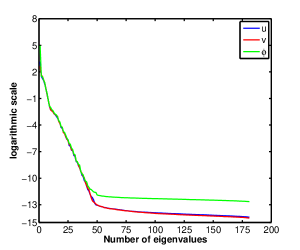
(a) Forward model snapshots only

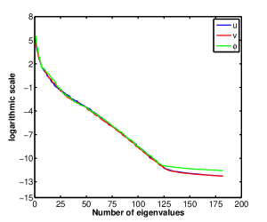
(b) Forward and adjoint models snapshots

Figure 1: The decay around of the singular values of the snapshots solutions for $u,v,\phi$ for $\Delta t=960s$ and integration time window of $3h$.

Forward snapshots consist in “predictor” and “corrector” state variables solutions ${\boldsymbol{w}}^{t_{i+1/2}}$, ${\boldsymbol{w}}^{t_{i}}$, $i=0,1,..,t_{f}-1$ and ${\boldsymbol{w}}^{t_{f}}$ obtained by solving the two steps forward ADI SWE model. The adjoint snapshots include the “predictor” and “corrector” adjoint solutions ${\bf\lambda}_{\bf w}^{t_{i-1/2}},~{}{\bf\lambda}_{\bf w}^{t_{i}},~{}i=1,2,.,t_{f}$ and ${\bf\lambda}_{\bf w}^{t_{0}}$ as well as other two additional intermediary solutions computed by the full adjoint model. An appendix is included providing details about the ADI SWE forward and adjoint models equations.

Next we compute the POD truncation relative errors for all three variables of reduced SWE models using the following norm at the initial time $t_{0}$

$$E_{\bar{\bf w}}=\frac{\|{\bar{\boldsymbol{w}}}^{t_{0}}-{\bar{\boldsymbol{w}}}^{t_{0}}_{\textsc{rom}}\|_{2}}{\|{\bar{\boldsymbol{w}}}^{t_{0}}\|_{2}},\quad E_{{\bar{\lambda}}_{\bf w}}=\frac{\|{{\bar{\lambda}}_{{\bf w}}}^{t_{0}}-{{\bar{\lambda}}_{{\bf w}^{ROM}}^{t_{0}}}\|_{2}}{\|{{\bar{\lambda}}_{{\bf w}}}^{t_{0}}\|_{2}},$$ (27)

where ${\bar{\boldsymbol{w}}}$ and ${{\bar{\lambda}}_{\bf w}}$ are general variables and span the sets of SWE state variables $\{u,v,\phi\}$ and adjoint variables $\{\lambda_{u},\lambda_{v},\lambda_{\phi}\}$. ${\bar{\boldsymbol{w}}}_{\textsc{rom}}$ and ${{\bar{\lambda}}_{{\bf w}^{ROM}}}$ are the full solutions reconstructed from the reduced order variables. $\|\cdot\|_{2}$ defines an Euclidian norm. The results are given in table 3.

AR ARRA $E_{u}$ $9.91e$-$16$ $5.16e$-$7$ $E_{v}$ $1.48e$-$15$ $1e$-$6$ $E_{\phi}$ $9.93e$-$16$ $6.78e$-$9$ AR ARRA $E_{\lambda_{u}}$ $0.969$ $5.94e$-$9$ $E_{\lambda_{v}}$ $0.926$ $5.18e$-$9$ $E_{\lambda_{\phi}}$ $0.220$ $1.65e$-$9$

Table 3: Relative errors of forward (left) and adjoint (right) tensorial POD SWE initial conditions using AR and ARRA approaches.

We did not scale the input snapshots. This approach seems to favor the reduced adjoint model with more accurate solutions than the reduced forward model.

Even if AR reduced data assimilation does not require a full adjoint model we chose to display the reduced adjoint time averaged relative error as a measure of increased probability that the output local minimum is far away from the local minimum computed with the high-fidelity configuration. Figure 2 depicts the minimization performances of the tensorial POD SWE 4D-Var systems using different set of snapshots in comparison with the output of the full space ADI SWE 4D-Var system. The cost function and gradient values are normalized by dividing them with their initial values.

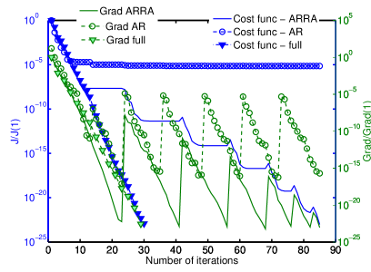
Figure 2: Tensorial POD/4DVAR ADI 2D Shallow water equations – Evolution of cost function and gradient norm as a function of the number of minimization iterations. The information from the adjoint equations has to be incorporated into POD basis.

Clearly the best POD basis construction strategy is “adjoint of reduced forward model + reduced order adjoint model” approach since the corresponding tensorial POD SWE 4D-Var achieved a cost function reduction close to the one obtained by the high-fidelity ADI SWE 4D-Var. One may notice that $6$ POD bases recalculations were required to achieve the suboptimal solution since $6$ plateaus regions followed by $6$ peaks are visible on the cost function curve. If only forward trajectory snapshots are utilized for POD basis construction the cost function decay is modest achieving only $5$ orders of magnitude decrease despite of carrying out $13$ POD bases updates. This underlines that the “adjoint of reduced forward model” approach is not able to represent well the controlled dynamics in its reduced manifold leading to an suboptimal cost function value of $0.48e$+$02$. In the case of “adjoint of reduced forward model + reduced order adjoint model” strategy the suboptimal cost function value is $0.48e$-$14$ while the optimal cost function calculated by the high fidelity ADI SWE 4D-Var system is $0.65e$-$16$. Two additional measures of the minimization performances are presented in Table 4 where the relative errors of tensorial POD suboptimal solutions with respect to observations and optimal solution are displayed. The data are generated using

$$E_{{\bar{\boldsymbol{w}}}}^{*}=\frac{\|{\bar{\boldsymbol{w}}}^{*}-{\bar{\boldsymbol{w}}}^{*}_{\textsc{rom}}\|_{2}}{\|{\bar{\boldsymbol{w}}}^{*}\|_{2}},\quad E_{{\bar{\boldsymbol{w}}}}^{o}=\frac{\|{\bar{\boldsymbol{w}}}^{\rm obs}-{\bar{\boldsymbol{w}}}^{*}_{\textsc{rom}}\|_{2}}{\|{\bar{\boldsymbol{w}}}^{\rm obs}\|_{2}},$$ (28)

${{\bar{\boldsymbol{w}}}}^{*}$ being the optimal solution provided by the full 4D-Var data assimilation system and spans the set $\{u^{*},v^{*},\phi^{*}\}$ , ${\bar{\boldsymbol{w}}}^{\rm obs}$ is the observation vector that spans the set $\{u^{\rm obs},v^{\rm obs},\phi^{\rm obs}\}$ and ${\bar{\boldsymbol{w}}^{*}}_{\textsc{rom}}$ is the sub-optimal solution proposed by the reduced 4D-Var systems and can take each of the following $\{{u^{\textsc{rom}}}^{*},{v^{\textsc{rom}}}^{*},{\phi^{\textsc{rom}}}^{*}\}$.

AR ARRA $E_{u}^{*}$ $1.57e$-$2$ $5.19e$-$11$ $E_{v}^{*}$ $1.81e$-$2$ $6.77e$-$11$ $E_{\phi}*$ $1.6e$-$2$ $5.96e$-$11$ AR ARRA $E_{u}^{o}$ $6.69e$-$5$ $2.39e$-$11$ $E_{v}^{o}$ $2.29e$-$4$ $8.71e$-$11$ $E_{\phi}^{o}$ $1.08e$-$6$ $3.7e$-$13$

Table 4: Relative errors of suboptimal solutions of reduced tensorial POD SWE systems using different snapshot sets and optimal solution (left) and observations (right). ^∗ denotes errors with respect to the optimal solution obtained using high-fidelity ADI SWE 4D-Var SWE system while ^o characterizes errors with respect to the observations.

We conclude that information from the full forward and adjoint solutions, as well as from the background term, must be included in the snapshots set used to derive the basis for Galerkin POD reduced order models. The smaller the error bounds $\varepsilon_{\textnormal{f}},~{}\varepsilon_{\textnormal{a}},~{}\varepsilon_{\textnormal{g}}$ in (19) are, the more accurate sub-optimal solutions are generated by the reduced order data assimilation systems. Next subsection includes experiments using only the ARRA strategy.

6.2 Reduced order POD based SWE 4D-Var data assimilation systems

This subsection is devoted to numerical experiments of the reduced SWE 4D-Var data assimilation systems introduced in subsection 5.2 using POD based models and discrete empirical interpolation method. In the on-line stage tensorial POD and POD/DEIM SWE forward models were shown to be faster than standard POD SWE forward model being $76\times$ and $450\times$ more efficient for more than $300,000$ variables (Ştefănescu et al. [35]). Moreover, a tensorial based algorithm was developed in [35] allowing the POD/DEIM SWE model to compute its off-line stage faster than the standard and tensorial POD approaches despite additional SVD calculations and other reduced coefficients calculations.

Consequently, one can assume that POD/DEIM SWE 4D-Var system would deliver suboptimal solutions faster than the other standard and tensorial POD data assimilation systems. The reduced Jacobians needed for solving the forward and adjoint reduced models are computed analytically for all three approaches. Since the derivatives computational complexity does not depend on full space dimension the corresponding adjoint models have similar CPU time costs. Thus, most of the CPU time differences will arise from the on-line stage of the reduced forward models and their off-line requirements.

6.2.1 POD/DEIM ADI SWE 4D-Var data assimilation system

Using nonlinear POD/DEIM approximation introduced in (8) we implement the reduced forward POD/DEIM ADI SWE obtained by projecting the ADI SWE equations onto the POD subspace. Then the reduced optimality conditions (13) are computed. For this choice of POD basis, the reduced POD/DEIM ADI SWE adjoint model is just the projection of the full adjoint model (5b) onto the reduced basis, and in consequence, they have similar algebraic structures requiring two different linear algebraic systems of equations to be solved at each time level (the algebraic form of ADI SWE adjoint model is given in appendix, see equations (35)-(36)).

The first reduced optimization test is performed for a mesh of $31\times 23$ points, a POD basis dimension of $k=50$, and $50$ and $180$ DEIM interpolation points are used. We obtain a cost function decrease of only $5$ orders of magnitude after $10$ POD bases updates and imposing a relaxed threshold of MXFUN $=100$ function evaluations per inner loop reduced optimization (see Figure 3a).

Thus we decide to incrementally increase the number of DEIM points until it reaches the number of space points and evaluate the reduced order POD/DEIM ADI SWE data assimilation system performances. However, our code is based on a truncated SVD algorithm that limits the number of POD modes of the nonlinear terms to a maximum of $2N_{t}-1$. This also constrains the maximum number of DEIM points to $2N_{t}-1$. Given this constraint, for the present space resolution $31\times 23$ points, we can not envisage numerical experiments where the number of DEIM points is equal to the number of space points since $N_{t}=91$.

In consequence we decrease the spatial resolution to $17\times 13$ points and perform the reduced optimization with increasing number of DEIM points and MXFUN $=20$ (see Figure 3b). For $m=165$, POD/DEIM nonlinear terms approximations are identical with standard POD representations since the boundary variables are not controlled. We notice that even for $m=135$ there is an important loss of performance since the cost function decreases by only $10^{-12}$ orders of magnitude in $178$ inner iterations while for $m=165$ (standard POD) the cost functions achieves a $10^{-23}$ orders of magnitude decrease in only $52$ reduced optimization iterations.

6.2.2 Adjoint and tangent linear POD/DEIM ADI SWE models verification tests

The initial level of root mean square error (RMSE) due to by truncation of POD expansion for $k=50$ and for a number of DEIM interpolation points $m=50$ at final time $t_{f}=3h$ are similar for all reduced order methods (see Table 5). It means that some of the nonlinear POD/DEIM approximations are more sensitive to changes in initial data during the optimization course while their nonlinear tensorial and standard POD counterparts proved to be more robust.

POD/DEIM tensorial POD standard POD $E_{u}$ $1.21e$-$7$ $1.2e$-$7$ $1.2e$-$7$ $E_{v}$ $7.6e$-$8$ $7.48e$-$8$ $7.48e$-$8$ $E_{\phi}$ $1.4e$-$7$ $1.36e$-$7$ $1.36e$-$7$

Table 5: RMSE of reduced order solutions of the forward SWE ROMS with respect to the full space ADI SWE state variables at final time $t_{f}=3h$ for the same initial conditions used for snapshots and POD basis generations. Number of mesh points is $n=17\times 13$, number of POD basis functions is $k=50$ and number of DEIM points is $m=50$.

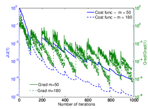
(a) Number of mesh points $31\times 23$

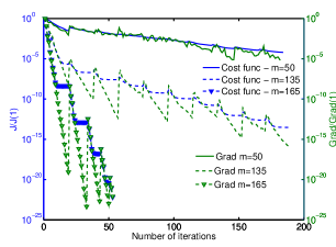
(b) Number of mesh points $17\times 13$

Figure 3: Standard POD/DEIM ADI SWE 4D-Var system – Evolution of cost function and gradient norm as a function of the number of minimization iterations for different number of mesh points and various number of DEIM points.

We verify the implementation of the POD/DEIM SWE 4D-Var system and the adjoint based gradient and the tangent linear model output agree with the finite difference approximations (see Figure 4a and [76, eq. (2.20)] for more details). The depicted values are obtained using

$$\rm{adj_{test}}=\frac{(J^{\textsc{pod}}({\bf\tilde{x}}_{0}+\delta{\bf\tilde{x}}_{0})-J^{\textsc{pod}}({\bf\tilde{x}}_{0}))}{<\nabla J^{\textsc{pod}}({\bf\tilde{x}}_{0}),\delta{\bf\tilde{x}}_{0}>_{2}}\quad\rm{tl_{test}}=\frac{\|\widetilde{\mathcal{M}}_{0,N_{t}}({\bf\tilde{x}}_{0}+\delta{\bf\tilde{x}}_{0})(N_{t})-\widetilde{\mathcal{M}}_{0,N_{t}}({\bf\tilde{x}}_{0})(N_{t})\|_{2}}{\|\widetilde{\bf M}_{0,N_{t}}(\delta{\bf\tilde{x}}_{0})(N_{t})\|_{2}},$$

where $\widetilde{\mathcal{M}}_{0,N_{t}}$, $\widetilde{\bf M}_{0,N_{t}}$ are the POD/DEIM forward and tangent linear models and $J^{\textsc{pod}}$ is computed using the POD/DEIM forward trajectory.

6.2.3 Hybrid POD/DEIM ADI SWE 4D-Var data assimilation system

Next we begin checking the accuracy of the POD/DEIM nonlinear terms during the optimization and compare them with the similar tensorial POD nonlinear terms (7). We found out that POD/DEIM nonlinear terms involving height ${\boldsymbol{\phi}}$, i.e. ${\tilde{F}}_{12},~{}{\tilde{F}}_{23},~{}{\tilde{F}}_{31},~{}{\tilde{F}}_{33}$ lose $2-3$ orders accuracy in comparison with tensorial nonlinear terms. Thus we replaced only these terms by their tensorial POD representations and the new hybrid POD/DEIM SWE system using $50$ DEIM interpolation points reached the expected performances (see Figure 4b).

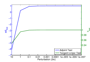
(a) Tangent Linear and Adjoint test

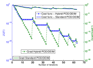
(b) Cost function and gradient decays

Figure 4: Tangent linear and adjoint test for standard POD/DEIM SWE 4D-Var system. Optimization performances of Standard POD/DEIM and Hybrid POD/DEIM 4D-Var ADI 2D shallow water equations for $n=17\times 13$.

Next we test the new hybrid POD/DEIM reduced data assimilation system using different POD basis dimensions and various numbers of DEIM points. For ROM optimization to deliver accurate suboptimal surrogate solutions similar to the output of full optimization one must increase the POD subspace dimension (see Figure 5a) for large number of mesh points configurations. Then we tested different configurations of DEIM points and for values of $m\geq 30$ the reduced optimization results are almost the same in terms of cost function decreases for $n=17\times 13$. Our findings were also confirmed by the relative errors accuracy of the suboptimal hybrid POD/DEIM SWE 4D-Var solutions with respect to the optimal solutions computed using high-fidelity ADI SWE 4D-Var system and observations (see Tables 6,7). We assumed that the background and observation errors are not correlated and their variances are equal to $1$.

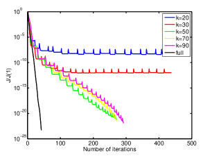
(a) Number of DEIM points $m=50$

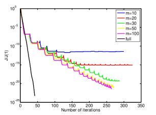
(b) Number of POD basis dimension $k=50$

Figure 5: Performances of hybrid POD/DEIM SWE DA system with various values of POD basis dimensions (a) and different number of interpolation points (b). The spatial configuration uses $n=61\times 45$ and maximum number of function evaluation per inner iteration is set MXFUN$=30$.

$k=20$ $k=30$ $k=50$ $k=70$ $k=90$ Full $E_{u}^{o}$ $1.03e$-$4$ $1.57e$-$6$ $4.1e$-$11$ $3.75e$-$11$ $2.1e$-$11$ $2.77e$-$12$ $E_{v}^{o}$ $4.04e$-$4$ $6.29e$-$6$ $1.72e$-$10$ $1.16e$-$10$ $8.55e$-$11$ $1.27e$-$11$ $E_{\phi}^{o}$ $2.36e$-$6$ $3.94e$-$8$ $1.09e$-$12$ $6.78e$-$13$ $2.3e$-$13$ $5.79e$-$14$

Table 6: Relative errors of suboptimal hybrid POD/DEIM SWE 4D-Var solutions with respect to observations. The number of DEIM interpolation points is held constant $m=50$ while $k$ is varied.

$m=10$ $m=20$ $m=30$ $m=50$ $m=100$ Full $E_{u}^{o}$ $4.28e$-$6$ $4.91e$-$8$ $4.15e$-$10$ $4.1e$-$11$ $3.08e$-$11$ $2.77e$-$12$ $E_{v}^{o}$ $6.88e$-$6$ $1.889e$-$7$ $1.54e$-$9$ $1.72e$-$10$ $1.25e$-$10$ $1.27e$-$11$ $E_{\phi}^{o}$ $7.15e$-$8$ $1.04e$-$9$ $7.79e$-$12$ $1.09e$-$13$ $7.39e$-$13$ $5.79e$-$14$

Table 7: Relative errors of suboptimal hybrid POD/DEIM SWE 4D-Var solutions with respect to observations. Different DEIM interpolation points are tested and $k$ is held constant $50$.

6.2.4 Computational cost comparison of reduced order 4D-Var data assimilation systems

This subsection is dedicated to performance comparisons between proposed optimization systems using reduced and full space configurations. We use different numbers of mesh points resolutions $31\times 23,~{}61\times 45,~{}101\times 71,~{}121\times 189,~{}151\times 111$ resulting in $1823,~{}7371,~{}20493,~{}28971$ and $48723$ control variables respectively. Various values of maximum number of function evaluations per each reduced minimization are also tested. We already proved that for increased number of POD basis dimensions the reduced data assimilation hybrid POD/DEIM ADI 4D-Var system leads to a cost function decrease almost similar with the one obtained by the full SWE 4D-Var system (see Figure 5a). Thus we are more interested to measure how fast the proposed data assimilation systems can reach the same threshold $\varepsilon_{3}$ in terms of cost function rate of decay.

Increasing the space resolution

The next experiment uses the following configuration: $n=61\times 45$ space points, number of POD basis modes $k=50$, MXFUN $=10$ and $\varepsilon_{3}=10^{-7}$. Figure 6 depicts the cost function evolution during hybrid POD/DEIM SWE 4D-Var, standard POD SWE 4D-Var and tensorial POD SWE 4D-Var minimizations versus number of iterations and CPU times. We notice that for $50$ DEIM points the hybrid POD/DEIM DA system requires $3$ additional POD basis updates to decrease the cost functional value below $10^{-7}$ in comparison with standard and tensorial POD DA systems. By increasing the number of DEIM points to $120$ the number of required POD basis recalculations is decreased by a factor of $2$ and the total number of reduced minimization iterations is reduced by $20$. The hybrid POD/DEIM SWE 4D-Var system using $m=120$ is faster with $\approx 37s$ and $\approx 86s$ than both the tensorial and standard POD SWE 4D-Var systems.

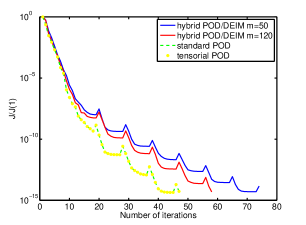
(a) Iteration performance

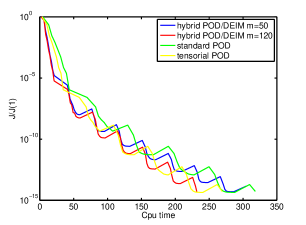
(b) Time performance

Figure 6: Number of minimization iterations and CPU time comparisons for the reduced order SWE DA systems vs. full SWE DA system. The spatial configuration uses $n=61\times 45$ and maximum number of function evaluation per inner iteration is set MXFUN$=10$.

Next we increase the number of spatial points to $n=151\times 111$ and use the same POD basis dimension $k=50$. MXFUN is set to $15$. The stopping criteria for all optimizations is $\|\mathcal{J}\|<\varepsilon_{3}=10^{-1}$. All the reduced order optimizations required two $POD$ basis recalculations and the hybrid POD/DEIM SWE 4D-Var needed one more iteration than the standard and tensorial POD systems (see Figure 7a). The hybrid POD/DEIM SWE 4D-Var system using $m=30$ is faster with $\approx 9s,92s,781s,4674s$ (by $1.01,~{}1.15,~{}2.31,~{}8.86$ times) than the hybrid POD/DEIM ($m=50$), tensorial POD, standard POD and full SWE 4D-Var data assimilation systems respectively (see Figure 7b).

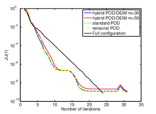
(a) Iteration performance

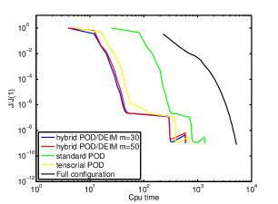
(b) Time performance

Figure 7: Number of iterations and CPU time comparisons for the reduced order SWE DA systems vs. full SWE DA system. The spatial configuration uses $n=151\times 111$ and maximum number of function evaluation per inner iteration is set MXFUN$=15$.

Table 8 displays the CPU times required by all the optimization methods to decrease the cost function values below a specific threshold $\varepsilon_{3}$ specific to each space configuration (row $2$ in table 8). The POD basis dimension is set to $k=30$. The bold values correspond to the best CPU time performances and some important conclusions can be drawn. There is no need for use of reduced optimization for $n=31\times 23$ or less since the full data assimilation system is faster. The hybrid POD/DEIM SWE 4D-Var using $50$ DEIM points is the most rapid optimization approach for numbers of space points larger than $61\times 45$. For $n=151\times 111$ it is $1.23,~{}2.27,~{}12.329$ faster than tensorial POD, standard POD and full SWE 4D-Var systems. We also notice that the CPU time speedup rates are directly proportional with the increase of the full space resolution dimensions.

Space points $31\times 23$ $61\times 45$ $101\times 71$ $121\times 89$ $151\times 111$ $\varepsilon_{3}$ $\|J\|<1.e$-$09$ $\|J\|<5.e$-$04$ $\|J\|<1.e$-$01$ $\|J\|<5$ $\|J\|<1e$+$03$ hybrid DEIM 50 48.771 63.345 199.468 358.17 246.397 hybrid DEIM 120 44.367 64.777 210.662 431.460 286.004 standard POD 63.137 131.438 533.052 760.462 560.619 tensorial POD 54.54 67.132 216.29 391.075 303.95 FULL 10.6441 117.02 792.929 1562.3425 3038.24

Table 8: CPU time for reduced optimization and full 4D-Var sharing the same stoping criterion $\|J\|<\varepsilon_{3}$. Number of POD modes is selected $30$ and MXFUN $=15$.

Increasing the POD basis dimension

Next we set the POD basis dimension to $50$ and the corresponding CPU times are described in Table $7$. Notice also that $\varepsilon_{3}$ values are decreased. The use of reduced optimization system is justified for $n>61\times 45$ where the hybrid POD/DEIM DA system using different numbers of DEIM points proves to be the fastest choice. For $151\times 111$ space points the hybrid POD/DEIM reduced optimization system is $1.15,~{}2.31,$ and $8.86$ times faster than tensorial POD, standard POD and full SWE 4D-Var systems respectively.

Space points $31\times 23$ $61\times 45$ $101\times 71$ $121\times 89$ $151\times 111$ $\varepsilon_{3}$ $\|J\|<1.e$-$14$ $\|J\|<1.e$-$07$ $\|J\|<1.e$-$04$ $\|J\|<5e$-$03$ $\|J\|<1e$-$01$ hybrid DEIM 30 214.78 288.627 593.357 499.676 594.04 hybrid DEIM 50 211.509 246.65 529.93 512.721 603.21 standard POD 190.572 402.208 1243.234 1315.573 1375.4 tensorial POD 269.08 311.106 585.509 662.95 685.57 FULL 14.1005 155.674 1057.715 2261.673 5268.7

Table 9: CPU time for reduced optimization and full 4D-Var sharing the same stoping criterion $\|J\|<\varepsilon_{3}$. Number of POD modes is selected $50$ and MXFUN $=15$.

Detailed computational cost analysis

Now we are able to describe the computational time required by each step of the high-fidelity and reduced optimization systems. We are using $151\times 111$ space points, POD basis dimension $k=50$, and number of DEIM points $m=30$. MXFUN is set to $15$ and $\varepsilon_{3}=10^{-1}$. For the full space 4D-Var system the line search and Hessian approximations are computational costly and are described separately (see table 10) while for reduced data assimilation systems these costs are very small being included in the reduced adjoint model CPU time.

Process	Time	#	Total
Solve full forward model	$\approx$ 80s	26x	$\approx$ 2080s
Solve full adjoint model	$\approx$ 76.45s	26x	$\approx$ 1987.7s
Other (Line Search, Hessian approx)	$\approx$ 46.165	26x	$\approx$ 1200.3s
Total full 4D-Var			$\approx$ 5268s

Table 10: The calculation times for solving the optimization problem using full 4D-Var for a number of mesh points of $151\times 111$. Stoping criterion $\|\mathcal{J}\|<10^{-1}$ is set.

The most expensive part of the Hybrid POD/DEIM 4D-Var optimization process (see table 11) occurs during the off-line stage and consists in the snapshots generation stage where the full forward and adjoint models are integrated in time. This is valid also for tensorial POD 4D-Var DA system (table 12) while in the case of standard POD 4D-Var system (table 13) the on-line stage is far more costly since the computational complexity of the corresponding reduced forward model still depends on the full space dimension.

Process	Time	#	Total
Off-line stage
Solve full forward model + nonlinear snap.	$\approx$ 80.88s	2x	$\approx$ 161.76s
Solve full adjoint model + nonlinear snap.	$\approx$ 76.45s	2x	$\approx$ 152.9s
SVD for state variables	$\approx$ 53.8	2x	$\approx$ 107.6s
SVD for nonlinear terms	$\approx$ 11.57	2x	$\approx$ 23.14s
DEIM interpolation points	$\approx$ 0.115	2x	$\approx$ 0.23s
POD/DEIM model coefficients	$\approx$ 1.06	2x	$\approx$ 2.12s
tensorial POD model coefficients	$\approx$ 8.8	2x	$\approx$ 17.6s
On-line stage
Solve ROM forward	$\approx$ 2s	33x	$\approx$ 66s
Solve ROM adjoint	$\approx$ 1.9s	33x	$\approx$ 62.69s
Total Hybrid POD/DEIM 4D-Var			$\approx$ 594.04s

Table 11: The calculation times for solving the optimization problem using Hybrid POD/DEIM 4D-Var for a number of mesh points of $151\times 111$, POD basis dimension $k=50$ and $30$ DEIM interpolation points.

The algorithm proposed in Ştefănescu and Navon [32, p.16] utilizes DEIM interpolation points, exploits the structure of polynomial nonlinearities and delivers fast tensorial calculations of POD/DEIM model coefficients. Consequently the hybrid POD/DEIM SWE 4D-Var systems has the fastest off-line stage among all proposed reduced data assimilation systems despite additional SVD calculations and other reduced coefficients computations.

Process	Time	#	Total
Off-line stage
Solve full forward model + nonlinear snap.	$\approx$ 80s	2x	$\approx$ 160s
Solve full adjoint model + nonlinear snap.	$\approx$ 76.45s	2x	$\approx$ 152.9s
SVD for state variables	$\approx$ 53.8s	2x	$\approx$ 107.6s
tensorial POD model coefficients	$\approx$ 23.735s	2x	$\approx$ 47.47s
On-line stage
Solve ROM forward	$\approx$ 4.9s	32x	$\approx$ 156.8s
Solve ROM adjoint	$\approx$ 1.9s	32x	$\approx$ 60.8s
Total Tensorial POD 4D-Var			$\approx$ 685.57s

Table 12: The calculation times for solving the optimization problem using Tensorial POD 4D-Var for a number of mesh points of $151\times 111$, and POD basis dimension $k=50$.

For all three reduced optimization systems the Jacobians are calculated analytically and their computations depend only on the reduced space dimension $k$. As a consequence, all the adjoint models have the same computational complexity and in the case of hybrid POD/DEIM SWE 4D-Var the on-line Jacobians computations rely partially on approximated tensors (40) calculated during the off-line stage while in the other two reduced order data assimilation systems exact tensorial POD model coefficients are used.

Process	Time	#	Total
On-line stage
Solve ROM forward	$\approx$ 26.523s	32x	$\approx$ 846.72s
Solve ROM adjoint	$\approx$ 1.9	32x	$\approx$ 60.8s
Total Standard 4D-Var			$\approx$ 1375.4s

Table 13: The calculation times for on-line stage of Standard POD 4D-Var for a number of mesh points of $151\times 111$ and POD basis dimension $k=50$. The off-line stage is identical with the one in Tensorial POD 4D-Var system.

Varying the number of function evaluations per reduced minimization cycle

The reduced optimization data assimilation systems become slow if it is repeatedly required to project back to the high fidelity model and reconstruct the reduced POD subspace. Thus, we compare the CPU times obtained by our reduced data assimilation systems using at most $10,~{}15,$ and $20$ function evaluations per reduced minimization cycle. The results for $k=30$ (see Table 14) shows that no more than $15$ function evaluations should be allowed for each reduced minimization cycle and hybrid POD/DEIM data assimilation system using $30$ interpolation points provides the fastest solutions. While for $101\times 71$ number of space points $15$ function evaluations are required, for other spatial configurations MXFUN $=10$ is sufficient.

Space points MXFUN $\varepsilon_{3}$ DEIM points Method $31\times 23$ - $1.e$-$9$ - Full $61\times 45$ 10 $5.e$-$04$ 30 Hybrid POD/DEIM $101\times 71$ 15 $1.e$-$01$ 30 Hybrid POD/DEIM $121\times 89$ 10 $5$ 30 Hybrid POD/DEIM $151\times 111$ 10 $1e$+$03$ 30 Hybrid POD/DEIM

Table 14: The fastest optimization data assimilation systems for various number of spatial points and different MXFUN values. Number of POD modes is $k=30$.

For POD basis dimension $k=50$, we discover that more function evaluations are needed during the inner reduced minimizations in order to obtain the fastest CPU times and MXFUN should be set to $15$. More DEIM points are also required as we notice in Table 15. Thus we can conclude that MXFUN should be increased with the decrease of $\varepsilon_{3}$ and increase of dimension of POD basis.

Space points MXFUN $\varepsilon_{3}$ DEIM points Method $31\times 23$ - $1.e$-$14$ - Full $61\times 45$ - $1.e$-$7$ - Full $101\times 71$ 15 $1.e$-$04$ 50 Hybrid POD/DEIM $121\times 89$ 15 $5.e$-$3$ 50 Hybrid POD/DEIM $151\times 111$ 15 $1.e$-$1$ 50 Hybrid POD/DEIM

Table 15: The fastest optimization data assimilation systems for various number of spatial points and different MXFUN values. Number of POD modes is $k=50$.

We conclude that hybrid POD/DEIM SWE 4D-Var system delivers the fastest suboptimal solutions and is far more competitive in terms of CPU time than the full SWE data assimilation system for space resolutions larger than $61\times 45$ points. Hybrid POD/DEIM SWE 4D-Var is at least two times faster than standard POD SWE 4D-Var for $n\geq 101\times 71$.

6.2.5 Accuracy comparison of reduced 4D-Var data assimilation suboptimal solutions

In terms of suboptimal solution accuracy, the hybrid POD/DEIM delivers similar results as tensorial and standard POD SWE 4D-Var systems (see tables 16, 17, 18). The accuracy of the reduced order models is tested via relative norms introduced in (27) at the beginning of reduced optimization algorithms and two different POD bases dimensions are tested, i.e. $k=30,~{}50$. To measure the suboptimal solutions accuracy we calculate the relative errors using $E_{{\bar{\boldsymbol{w}}}}^{*}$ defined in (28) and the corresponding values are depicted in the hybrid DEIM, sPOD and tPOD columns. MXFUN is set to $15$. We choose $\varepsilon_{3}=10^{-15}$ for all data assimilation systems and only $20$ outer iterations are allowed for all reduced 4D-Var optimization systems. For Hybrid POD/DEIM 4D-Var system we use $50$ DEIM interpolation points.

$n$ $E_{u}$ $E_{\lambda_{u}}$ hybrid DEIM sPOD tPOD $31\times 23$ $4.51e$-$5$ $5.09e$-$5$ $5.86e$-$8$ $9.11e$-$8$ $9.11e$-$8$ $61\times 45$ $1.55e$-$4$ $2.92e$-$4$ $2.4e$-$5$ $1.63e$-$5$ $1.63e$-$5$ $101\times 71$ $6.06e$-$4$ $6.56e$-$4$ $2.03e$-$4$ $1.83e$-$4$ $1.83e$-$4$ $121\times 89$ $9.88e$-$4$ $1.93e$-$3$ $1.16e$-$3$ $8.07e$-$4$ $8.07e$-$4$ $151\times 111$ $2.07e$-$3$ $2.97e$-$3$ $4.02e$-$3$ $4.2e$-$3$ $4.2e$-$3$ $E_{u}$ $E_{\lambda_{u}}$ hybrid DEIM sPOD tPOD $1.39e$-$6$ $1.87e$-$6$ $1.13e$-$10$ $2.51e$-$10$ $2.51e$-$10$ $1.58e$-$5$ $1.06e$-$5$ $2.16e$-$7$ $1.38e$-$7$ $1.38e$-$7$ $4.51e$-$5$ $4.76e$-$5$ $7.03e$-$6$ $5.14e$-$6$ $5.14e$-$6$ $7.17e$-$5$ $8.e$-$5$ $5.62e$-$5$ $3.15e$-$5$ $3.15e$-$5$ $1.02e$-$4$ $2.77e$-$4$ $1.59e$-$4$ $1.05e$-$4$ $1.05e$-$4$

Table 16: Reduced order forward and adjoint model errors vs. reduced order optimal solution errors for velocity component $u$ using $30$ (left) and $50$ (right) POD modes.

$n$ $E_{v}$ $E_{\lambda_{v}}$ hybrid DEIM sPOD tPOD $31\times 23$ $3.20e$-$5$ $4.06e$-$5$ $6.03e$-$8$ $9.95e$-$8$ $9.95e$-$8$ $61\times 45$ $3.13e$-$4$ $3.21e$-$4$ $3.75e$-$5$ $2.63e$-$5$ $2.63e$-$5$ $101\times 71$ $9.76e$-$4$ $5.71e$-$4$ $3.51e$-$4$ $2.93e$-$4$ $2.93e$-$4$ $121\times 89$ $1.37e$-$3$ $1.70e$-$3$ $1.38e$-$3$ $1.21e$-$3$ $1.21e$-$3$ $151\times 111$ $1.58$-$3$ $1.89e$-$3$ $6.21e$-$3$ $6.22e$-$3$ $6.22e$-$3$    $E_{v}$ $E_{\lambda_{v}}$ hybrid DEIM sPOD tPOD $7.54e$-$7$ $1.10e$-$6$ $1.25e$-$10$ $4.10e$-$10$ $4.10e$-$10$ $1.09e$-$5$ $9.71e$-$6$ $3.03e$-$7$ $2.82e$-$7$ $2.82e$-$7$ $3.05e$-$5$ $3.55e$-$5$ $8.32e$-$6$ $9.45e$-$6$ $9.45e$-$6$ $7.96e$-$5$ $8.12e$-$5$ $7.19e$-$5$ $6.85e$-$5$ $6.85e$-$5$ $1.06e$-$4$ $1.76e$-$4$ $2.95e$-$4$ $1.94e$-$4$ $1.94e$-$4$

Table 17: Reduced order forward and adjoint model errors vs. reduced order optimal solution errors for velocity component $v$ using $30$ (left) and $50$ (right) POD modes.

$n$ $E_{\phi}$ $E_{\lambda_{\phi}}$ hybrid DEIM sPOD tPOD $31\times 23$ $4.38e$-$5$ $4.16e$-$5$ $1.12e$-$7$ $1.83e$-$7$ $1.83e$-$7$ $61\times 45$ $1.84e$-$4$ $4.54e$-$4$ $5.63e$-$5$ $3.34e$-$5$ $3.34e$-$5$ $101\times 71$ $2.21e$-$3$ $3.16e$-$3$ $6.60e$-$4$ $6.45e$-$4$ $6.45e$-$4$ $121\times 89$ $5.60e$-$3$ $4.38e$-$3$ $2.88e$-$3$ $2.54e$-$3$ $2.54e$-$3$ $151\times 111$ $9.04e$-$3$ $1.2e$-$2$ $8.54e$-$3$ $8.46e$-$3$ $8.46e$-$3$     $E_{\phi}$ $E_{\lambda_{\phi}}$ hybrid DEIM sPOD tPOD $1.59e$-$6$ $1.04e$-$6$ $1.12e$-$10$ $2.87e$-$10$ $2.87e$-$10$ $9.58e$-$6$ $9.e$-$6$ $1.80e$-$7$ $2.37e$-$7$ $2.37e$-$7$ $3.52e$-$5$ $4.49e$-$5$ $7.60e$-$6$ $1.04e$-$5$ $1.04e$-$5$ $7.84e$-$5$ $1.03e$-$4$ $5.56$e-$5$ $5.04e$-$5$ $5.04e$-$5$ $1.8e$-$4$ $2.77e$-$4$ $2.76e$-$4$ $2.75e$-$4$ $2.75e$-$4$

Table 18: Reduced order forward and adjoint model errors vs. reduced order optimal solution errors for geopotential $\phi$ using $30$ (left) and $50$ (right) POD modes.

The suboptimal errors of all reduced optimization systems $E_{{\bar{\boldsymbol{w}}}}^{*}$ are well correlated with the relative errors of the reduced order models $E_{\bar{\bf w}}$ and $E_{{\bar{\lambda}}_{\bf w}}$ (27), having correlation coefficients higher than $0.85$. However the correlation coefficients between reduced adjoint model errors and suboptimal errors are larger than $0.9$ which confirm the a-priori error estimation results of Hinze and Volkwein [53] developed for linear-quadratic optimal problems. It states that error estimates for the adjoint state yield error estimates of the control. Extension to nonlinear-quadratic optimal problems is desired and represents subject of future research. In addition, an a-posteriori error estimation apparatus is required by the hybrid POD/DEIM SWE system to guide the POD basis construction and to efficiently select the number of DEIM interpolation points.

The suboptimal solutions delivered by the ROM DA systems equipped with BFGS algorithm are accurate and comparable with the optimal solution computed by the full DA system. In the future we plan to enrich the reduced data assimilation systems by implementing a trust region algorithm (see Arian et al. [10]). It has an efficient strategy for updating the POD basis and it is well known for its global convergence properties.

7 Conclusions

This work studies the use of reduced order modeling to speed up the solution of variational data assimilation problems with nonlinear dynamical models. The novel ARRA framework proposed herein guarantees that the Karush-Kuhn-Tucker conditions of the reduced order optimization problem accurately approximate the corresponding first order optimality conditions of the full order problem. In particular, accurate low-rank approximations of the adjoint model and of the gradient equation are obtained in addition to the accurate low-rank representation of the forward model. The construction is validated by an error estimation result.

The choice of the reduced basis in the ARRA approach depends on the type of projection employed. For a pure Petrov-Galerkin projection the test POD basis functions of the forward model coincide with the trial POD basis functions of the adjoint model; and similarly, the adjoint test POD basis functions coincide with the forward trial POD basis functions. Moreover the trial POD basis functions of the adjoint model should also include gradient information. It is well known that pure Petrov-Galerkin reduced order models can exhibit severe numerical instabilities, therefore stabilization strategies have to be included with this type of reduced data assimilation system [7, 22].

In the ARRA Galerkin projection approach the same reduced order basis has to represent accurately the full order forward solution, the full order adjoint solution, and the full order gradient. The Galerkin POD bases are constructed from the dominant eigenvectors of the correlation matrix of the aggregated set of vectors containing snapshots of the full order forward and adjoint models, as well as the full order background term. This reduced bases selection strategy is not limited to POD framework. It extends easily to every type of reduced optimization involving projection-based reduced order methods such the reduced basis approach.

Numerical experiments using tensorial POD SWE 4D-Var data assimilation system based on Galerkin projection and different type of POD bases support the proposed approach. The most accurate suboptimal solutions and the fastest decrease of the cost function are obtained using full forward and adjoint trajectories and background term derivative as snapshots for POD basis generation. If only forward model information is included into the reduced manifold the cost function associated with the data assimilation problem decreases by only five orders of magnitude during the optimization process. Taking into account the adjoint and background term derivative information leads to a decrease of the cost function by twenty orders of magnitude and the results of the reduced-order data assimilation system are similar with the ones obtained with the Full order SWE 4D-Var DA system. This highlights the importance of choosing appropriate reduced-order bases.

A numerical study of how the choice of reduced order technique impacts the solution of the inverse problem is performed. We consider for comparison standard POD, tensorial POD and standard POD/DEIM. For the first time POD/DEIM is employed to construct a reduced-order data assimilation system for a geophysical two-dimensional flow model. All reduced-order DA systems employ a Galerkin projection and the reduced-order bases use information from both forward and dual solutions and the background term derivative. The POD/DEIM approximations of several nonlinear terms involving the height field partially lose their accuracy during the optimization. It suggests that POD/DEIM reduced nonlinear terms are sensitive to input data changes and the selection of interpolation points is no longer optimal. On-going research focuses on increasing the robustness of DEIM for optimization applications. The number of DEIM points must be taken closer to the number of space points for accurate sub-optimal solutions leading to slower on-line stage. The reduced POD/DEIM approximations of the aforementioned nonlinear terms are replaced with tensorial POD representations. This new hybrid POD/DEIM SWE 4D-Var DA system is accurate and faster than other standard and tensorial POD SWE 4D-Var systems. Numerical experiments with various POD basis dimensions and numbers of DEIM points illustrate the potential of the new reduced-order data assimilation system to reduce CPU time.

For a full system spatial discretization with $151\times 111$ grid points the hybrid POD/DEIM reduced data assimilation system is approximately ten times faster then the full space data assimilation system. This rate increases in proportion to the increase in the number of grid points used in the space discretization. Hybrid POD/DEIM SWE 4D-Var is at least two times faster than standard POD SWE 4D-Var for numbers of space points larger or equal to $101\times 71$. This illustrates the power of DEIM approach not only for reduced-order forward simulations but also for reduced-order optimization.

Our results reveal a relationship between the size of the POD basis and the magnitude of the cost function error criterion $\varepsilon_{3}$. For a very small $\varepsilon_{3}$ the reduced order data assimilation system may not able to sufficiently decrease the cost function. The optimization stops only when the maximum number of outer loops is reached or the high-fidelity gradient based optimality condition is satisfied . In consequence, one must carefully select $\varepsilon_{3}$ since the ROM DA machinery is more efficient when the number of outer loops is kept small. In addition, the number of function evaluations allowed during the inner minimization phase should be increased with the decrease of $\varepsilon_{3}$ and increase of POD basis dimension in order to speed up the reduced optimization systems.

Future work will consider Petrov-Galerkin stabilization approaches [22, 7]. Moreover, we will focus on a generalized DEIM framework [34] to approximate operators since faster reduced Jacobian computations will further decrease the computational complexity of POD/DEIM reduced data assimilation systems. We will also address the impact of snapshots scaling in the accuracy of the sub-optimal solution. One approach would be to normalize each snapshot and to use vectors of norm one as input for the singular value decompositions.

We intend to extend our reduced-order data assimilation systems by implementing a trust region algorithm to guide the re-computation of the bases. On-going work of the authors seeks to develop a-priori and a-posteriori error estimates for the reduced-order optimal solutions, and to use a-posteriori error estimation apparatus to guide the POD basis construction and to efficiently select the number of DEIM interpolation points.

Appendix

This appendix contains a symbolic representation of the Gustafsson’s nonlinear ADI finite difference shallow water equations schemes defined in (22) and the formulas of SWE tensors required by all three studied reduced order models.

Gustafsson’s nonlinear ADI finite difference shallow water equations models

ADI SWE scheme requires two steps to solve for ${\boldsymbol{u}}^{N+1},\quad{\boldsymbol{v}}^{N+1},\quad{\boldsymbol{\phi}}^{N+1}$.

First step - get solution at $t_{N+\frac{1}{2}}$

$$\begin{split}&D_{-t}{\bf u}^{{N+\frac{1}{2}}}=-F_{11}({\bf u}^{N+\frac{1}{2}})-F_{12}(\bm{{\phi}}^{N+\frac{1}{2}})-F_{13}({\bf u}^{N},{\bf v}^{N})+{\bf F}\odot{\bf v}^{N},\\ &D_{-t}{\bf v}^{{N+\frac{1}{2}}}=-F_{21}({\bf u}^{N+\frac{1}{2}})-F_{22}({\bf v}^{N})-F_{23}(\bm{{\phi}}^{N})-{\bf F}\odot{\bf u}^{N+\frac{1}{2}},\\ &D_{-t}{\bm{{\phi}}}^{{N+\frac{1}{2}}}=-F_{31}({\bf u}^{N+\frac{1}{2}},\bm{{\phi}}^{N+\frac{1}{2}})-F_{32}({\bf u}^{N+\frac{1}{2}},\bm{{\phi}}^{N+\frac{1}{2}})-F_{33}({\bf v}^{N},\bm{{\phi}}^{N})-F_{34}({\bf v}^{N},\bm{{\phi}}^{N}),\end{split}$$ (29)

where $D_{-t}^{{N+\frac{1}{2}}}{\bf w}$ is the backward in time difference operator, ${\bf w}=({\bf u},{\bf v},{\bm{\phi}})$, $\odot$ is the component-wise multiplication operator, ${\bf F}=[\underbrace{{\bf f},{\bf f},..,{\bf f}}_{N_{x}}]$ stores Coriolis components ${\bf f}=[f(y_{j})]_{j=1,2,..,N_{y}}$ while the nonlinear terms $F_{i,j}$ are defined in (25).

Second step - get solution at $t_{N+1}$

$$\begin{split}&D_{-t}{\bf u}^{{N+1}}=-F_{13}({\bf u}^{N+1},{\bf v}^{N+1})+{\bf F}\odot{\bf v}^{N+1}-F_{11}({\bf u}^{N+\frac{1}{2}})-F_{12}(\bm{{\phi}}^{N+\frac{1}{2}}),\\ &D_{-t}{\bf v}^{{N+1}}=-F_{22}({\bf v}^{N+1})-F_{23}(\bm{{\phi}}^{N+1})-F_{21}({\bf u}^{N+\frac{1}{2}})-{\bf F}\odot{\bf u}^{N+\frac{1}{2}},\\ &D_{-t}{\bm{{\phi}}}^{{N+1}}=-F_{33}({\bf v}^{N+1},\bm{{\phi}}^{N+1})-F_{34}({\bf v}^{N+1},\bm{{\phi}}^{N+1})-F_{31}({\bf u}^{N+\frac{1}{2}},\bm{{\phi}}^{N+\frac{1}{2}})-F_{32}({\bf u}^{N+\frac{1}{2}},\bm{{\phi}}^{N+\frac{1}{2}}).\end{split}$$ (30)

The nonlinear systems of algebraic equations (29) and (30) are solved using quasi-Newton method, thereby we rewrite them in the form

$${\bf g}({\boldsymbol{w}})=0,\quad{\bf g}({\boldsymbol{w}})=\left(\begin{array}[]{c}{g_{1}({\boldsymbol{w}}^{N+\frac{1}{2}},{\boldsymbol{w}}^{N})}\\ {g_{2}({\boldsymbol{w}}^{N+1},{\boldsymbol{w}}^{N+\frac{1}{2}})}\\ \end{array}\right),$$ (31)

where ${g_{1}}$ and ${g_{2}}$ represent systems (29) and (30). The corresponding iterative Newton steps are

$$\begin{split}&{\delta\boldsymbol{w}}^{N+\frac{1}{2}}=-\frac{\partial g_{1}}{\partial w^{N+\frac{1}{2}}}({\boldsymbol{w}}^{N+\frac{1}{2}},{\boldsymbol{w}}^{N})^{-1}g_{1}({\boldsymbol{w}}^{N+\frac{1}{2}},{\boldsymbol{w}}^{N}),\\ &{\delta\boldsymbol{w}}^{N+1}=-\frac{\partial g_{2}}{\partial w^{N+1}}({\boldsymbol{w}}^{N+1},{\boldsymbol{w}}^{N+\frac{1}{2}})^{-1}g_{2}({\boldsymbol{w}}^{N+1},{\boldsymbol{w}}^{N+\frac{1}{2}}).\end{split}$$ (32)

We avoid evaluating the Jacobian matrices at every iteration by proposing a Quasi-Newton approach:

$$\begin{split}&{\delta\boldsymbol{w}}^{N+\frac{1}{2}}=-\frac{\partial g_{1}}{\partial w^{N+\frac{1}{2}}}({\boldsymbol{w}}^{N})^{-1}g_{1}({\boldsymbol{w}}^{N+\frac{1}{2}},{\boldsymbol{w}}^{N}),\\ &{\delta\boldsymbol{w}}^{N+1}=-\frac{\partial g_{2}}{\partial w^{N+1}}({\boldsymbol{w}}^{N+\frac{1}{2}})^{-1}g_{2}({\boldsymbol{w}}^{N+1},{\boldsymbol{w}}^{N+\frac{1}{2}}).\end{split}$$ (33)

Then, we linearize the discrete models using the total variation method [33, eq. (3.2)] and obtain the tangent linear model by subtracting the set of equations (31) using different arguments $({\boldsymbol{w}}^{N+\frac{1}{2}},{\boldsymbol{w}}^{N})$ and $({\boldsymbol{w}}^{N+1},{\boldsymbol{w}}^{N+\frac{1}{2}})$ and their increments $({\boldsymbol{w}}^{N+\frac{1}{2}}+{\delta\boldsymbol{w}}^{N+\frac{1}{2}},{\boldsymbol{w}}^{N}+{\delta\boldsymbol{w}}^{N})$ and $({\boldsymbol{w}}^{N+1}+{\delta\boldsymbol{w}}^{N+1},{\boldsymbol{w}}^{N+\frac{1}{2}}+{\delta\boldsymbol{w}}^{N+\frac{1}{2}})$

$$\left\{\begin{split}&\frac{\partial g_{1}}{\partial w^{N+\frac{1}{2}}}({\boldsymbol{w}}^{N}){\delta\boldsymbol{w}}^{N+\frac{1}{2}}=-\frac{\partial g_{1}}{\partial w^{N}}({\boldsymbol{w}}^{N}){\delta\boldsymbol{w}}^{N},\\ &\frac{\partial g_{2}}{\partial w^{N+1}}({\boldsymbol{w}}^{N+\frac{1}{2}}){\delta\boldsymbol{w}}^{N+1}=-\frac{\partial g_{2}}{\partial w^{N+\frac{1}{2}}}({\boldsymbol{w}}^{N+\frac{1}{2}}){\delta\boldsymbol{w}}^{N+\frac{1}{2}},\\ \end{split}\right.$$ (34)

and ${\delta\boldsymbol{w}}=({\delta\boldsymbol{u}},{\delta\boldsymbol{v}},{\delta\boldsymbol{\phi}})$ are the tangent linear unknowns.

The adjoint model is obtained by transposing (34)

First step - get solution at $t_{N+\frac{1}{2}}$

$$\left\{\begin{split}&\big{[}\frac{\partial g_{2}}{\partial w^{N+1}}({\boldsymbol{w}}^{N+\frac{1}{2}})\big{]}^{T}{\boldsymbol{z}}^{N+1}={\boldsymbol{\lambda}}^{N+1},\\ &{\boldsymbol{\lambda}}^{N+\frac{1}{2}}=\big{[}-\frac{\partial g_{2}}{\partial w^{N+\frac{1}{2}}}({\boldsymbol{w}}^{N+\frac{1}{2}})\big{]}^{T}{\boldsymbol{z}}^{N+1}.\end{split}\right.$$ (35)

Second step - get solution at $t_{N}$

$$\left\{\begin{split}&\big{[}\frac{\partial g_{1}}{\partial w^{N+\frac{1}{2}}}({\boldsymbol{w}}^{N})\big{]}^{T}{\boldsymbol{z}}^{N+\frac{1}{2}}={\boldsymbol{\lambda}}^{N+\frac{1}{2}},\\ &{\boldsymbol{\lambda}}^{N}=\big{[}-\frac{\partial g_{1}}{\partial w^{N}}({\boldsymbol{w}}^{N})\big{]}^{T}{\boldsymbol{z}}^{N+\frac{1}{2}},\end{split}\right.$$ (36)

where ${\boldsymbol{\lambda}}=({\boldsymbol{\lambda}_{u}},{\boldsymbol{\lambda}_{v}},{\boldsymbol{\lambda}_{\phi}})$ are the adjoint unknowns and ${\boldsymbol{z}}$ is an intermediary variable. By $\big{[}\frac{\partial g_{1}}{\partial w^{N+\frac{1}{2}}}({\boldsymbol{w}}^{N})\big{]}^{T}$ we denote the transpose of Jacobian $\frac{\partial g_{1}}{\partial w^{N+\frac{1}{2}}}({\boldsymbol{w}}^{N})$.

SWE tensors

The Jacobian matrices required by the quasi-Newton method to solve the standard POD and tensorial POD reduced models are the same and their formulations are obtained analytically. The Jacobian matrices depend on specific tensors computed based on the general formula introduced in (7). In the case of standard POD/DEIM SWE model we approximate these tensors using the algorithm introduced in [35, p.7]. For each nonlinear SWE term (25) we need to define one tensor. Before introducing their formulas we first define the POD bases and their derivatives. We recall that the discrete full space dimension is $n$ and for each state variable we compute the test and trial functions assuming the bases have the same dimension $k$.

$$\begin{split}&{\bf U},~{}{\bf V},~{}{\bf\Phi},~{}{\bf W^{u}},~{}{\bf W^{v}},~{}{\bf W^{\phi}}\in\mathbb{R}^{n\times k}\\ &{\bf U_{x}}=A_{x}{\bf U}\in\mathbb{R}^{n\times k},~{}{\bf V_{x}}=A_{x}{\bf V}\in\mathbb{R}^{n\times k},~{}{\bf\Phi_{x}}=A_{x}{\bf\Phi}\in\mathbb{R}^{n\times k},\\ &{\bf U_{y}}=A_{y}{\bf U}\in\mathbb{R}^{n\times k},~{}{\bf V_{y}}=A_{y}{\bf V}\in\mathbb{R}^{n\times k},~{}{\bf\Phi_{y}}=A_{y}{\bf\Phi}\in\mathbb{R}^{n\times k},\\ \end{split}$$ (37)

where $A_{x},A_{y}\in\mathbb{R}^{n\times n}$ are constant coefficient matrices for discrete first-order and second-order differential operators which incorporate the boundary conditions.

The SWE tensors formulas for the standard POD and tensorial POD reduced order models are

$$\begin{split}&T^{f}=\left(T^{f}_{i,j,l}\right)_{i,j,l=1,..,k}\in\mathbb{R}^{k\times k\times k},~{}f=11,12,13,21,22,23,31,32,33,34.\\ &T^{11}_{i,j,l}=\sum_{r=1}^{n}W^{u}_{r,i}U_{r,j}{U_{x}}_{r,l},\quad T^{12}_{i,j,l}=\sum_{r=1}^{n}W^{u}_{r,i}\Phi_{r,j}{\Phi_{x}}_{r,l},\quad T^{13}_{i,j,l}=\sum_{r=1}^{n}W^{u}_{r,i}V_{r,j}{U_{y}}_{r,l},\\ &T^{21}_{i,j,l}=\sum_{r=1}^{n}W^{v}_{r,i}U_{r,j}{V_{x}}_{r,l},\quad T^{22}_{i,j,l}=\sum_{r=1}^{n}W^{v}_{r,i}V_{r,j}{V_{y}}_{r,l},\quad T^{23}_{i,j,l}=\sum_{r=1}^{n}W^{v}_{r,i}\Phi_{r,j}{\Phi_{y}}_{r,l},\\ &T^{31}_{i,j,l}=\sum_{r=1}^{n}W^{\phi}_{r,i}\Phi_{r,j}{U_{x}}_{r,l},\quad T^{32}_{i,j,l}=\sum_{r=1}^{n}W^{\phi}_{r,i}U_{r,j}{\Phi_{x}}_{r,l},\quad T^{33}_{i,j,l}=\sum_{r=1}^{n}W^{\phi}_{r,i}\Phi_{r,j}{V_{y}}_{r,l},\\ &T^{34}_{i,j,l}=\sum_{r=1}^{n}W^{\phi}_{r,i}V_{r,j}{\Phi_{y}}_{r,l}.\\ \end{split}$$ (38)

In the case of standard POD/DEIM SWE model, the above tensors are computed by making use of the DEIM approximation of the nonlinear terms, resulting in an off-line stage that is faster [35, Figure 8(b)] than the versions proposed by standard POD and tensorial POD, even if additional SVD decompositions and low-rank terms are calculated.

To render the manuscript as self-contained as possible we describe the methodology used for computing one POD/DEIM tensor. For example, the POD/DEIM reduced nonlinear version of $F_{11}$ defined in (25) is given by

$${\tilde{F}}_{11}\approx\underbrace{{\bf W^{u}}^{T}{\bf F}_{11}^{\rm{POD}}(P^{T}{\bf F}_{11}^{\rm{POD}})^{-1}}_{k\times m}\underbrace{\left(P^{T}{\bf U}{\bf\tilde{x}}\odot P^{T}{\bf U_{x}}{\bf\tilde{x}}\right)}_{m\times 1},$$ (39)

where ${\bf F}_{11}^{\rm{POD}}\in\mathbb{R}^{n\times m}$ is the POD basis of dimension $m$ obtained from the snapshots of the SWE nonlinear term $F_{11}$ (for more details see also the general form of POD/DEIM expansion (8)). Let us denote by $E={{\bf W^{u}}^{T}{\bf F}_{11}^{\rm{POD}}(P^{T}{\bf F}_{11}^{\rm{POD}})^{-1}}\in\mathbb{R}^{k\times m}$, ${\bf U}^{m}=P^{T}{\bf U}\in\mathbb{R}^{m\times k}$ and ${\bf U_{x}}^{m}=P^{T}{\bf U_{x}}\in\mathbb{R}^{m\times k}$, than the associated tensor computed during the POD/DEIM off-line stage is

$${T^{11}}^{\rm{DEIM}}_{i,j,l}=\sum_{r=1}^{m}E_{i,r}U^{m}_{j,r}{U_{x}}^{m}_{r,l},\quad i,j,l=1,..,k.$$ (40)

In comparison with the formula used by standard and tensorial POD (38), we notice that the summation spans only the location of DEIM points instead of entire discrete space. For completeness, we recall that $n$ is the size of the full discrete space, $k$ is the size of reduced order model and $m$ is the number of DEIM points.

References

- A. et al. [2014] Caiazzo A., T. Iliescu, V. John, and S. Schyschlowa. A numerical investigation of velocity–pressure reduced order models for incompressible flows. Journal of Computational Physics, 259(0):598 – 616, 2014.
- Afanasiev and Hinze [2001] K. Afanasiev and M. Hinze. Adaptive Control of a Wake Flow Using Proper Orthogonal Decomposition. Lecture Notes in Pure and Applied Mathematics, 216:317–332, 2001.
- Alexe [2011] M. Alexe. Adjoint-based space-time adaptive solution algorithms for sensitivity analysis and inverse problems. PhD thesis, Computer Science Department, Virginia Tech, 2011.
- Alexe and Sandu [2014] Mihai Alexe and Adrian Sandu. Space–time adaptive solution of inverse problems with the discrete adjoint method. Journal of Computational Physics, 270:21–39, 2014.
- Altaf et al. [2013] M.U. Altaf, M.E. Gharamti, A.W. Heemink, and I. Hoteit. A reduced adjoint approach to variational data assimilation. Computer Methods in Applied Mechanics and Engineering, 254:1–13, 2013.
- Ambrozic [2013] M. Ambrozic. A Study of Reduced Order 4D-VAR with a Finite Element Shallow Water Model. Master’s thesis, Delft University of Technology, Netherlands, 2013.
- Amsallem and Farhat [2012] D. Amsallem and C. Farhat. Stabilization of projection-based reduced-order models. Int. J. Numer. Meth. Engng., 91:358–377, 2012.
- Amsallem et al. [2013] D. Amsallem, M. Zahr, Y. Choi, and C. Farhat. Design Optimization Using Hyper-Reduced-Order Models. Technical report, Stanford University, 2013.
- Arian et al. [2000a] E. Arian, M. Fahl, and E.W. Sachs. Trust-region proper orthogonal decomposition for flow control. ICASE: Technical Report 2000-25, 2000a.
- Arian et al. [2000b] E. Arian, M. Fahl, and E.W. Sachs. Trust-region proper orthogonal decomposition for flow control. Institute for Computer Applications in Science and Engineering, Hampton VA, 2000b.
- Atwell and King [2001] J.A. Atwell and B.B. King. Proper orthogonal decomposition for reduced basis feedback controllers for parabolic equations. Mathematical and Computer Modelling, 33(1–3):1–19, 2001.
- Atwell and King [2004] J.A. Atwell and B.B. King. Reduced Order Controllers for Spatially Distributed Systems via Proper Orthogonal Decomposition. SIAM J. Sci. Comput., 26(1):128–151, 2004.
- Barrault et al. [2004] M. Barrault, Y. Maday, N.C. Nguyen, and A.T. Patera. An ’empirical interpolation’ method: application to efficient reduced-basis discretization of partial differential equations. Compt. Rend. Math., 339(9):667–672, 2004.
- Barrett et al. [1994] R. Barrett, M. Berry, T. F. Chan, J. Demmel, J. Donato, J. Dongarra, V. Eijkhout, R. Pozo, C. Romine, and H. Van der Vorst. Templates for the Solution of Linear Systems: Building Blocks for Iterative Methods, 2nd Edition. SIAM, Philadelphia, PA, 1994.
- Baumann [2013] M.M. Baumann. Nonlinear Model Order Reduction using POD/DEIM for Optimal Control of Burgers equation. Master’s thesis, Delft University of Technology, Netherlands, 2013.
- Becker and Vexler [2005] R. Becker and B. Vexler. Mesh refinement and numerical sensitivity analysis for parameter calibration of partial differential equations. J. Comput. Phys., 206(1):95–110, 2005.
- Bergmann and Cordier [2007] M. Bergmann and L. Cordier. Drag minimization of the cylinder wake by trust-region proper orthogonal decomposition. Notes on Numerical Fluid Mechanics and Multidisciplinary Design, 95(16):309–324, 2007.
- Bergmann and Cordier [2008] M. Bergmann and L. Cordier. Optimal control of the cylinder wake in the laminar regime by trust-region methods and pod reduced-order models. Journal of Computational Physics, 227(16):7813–7840, 2008.
- Bergmann et al. [2005] M. Bergmann, L. Cordier, and J.P. Brancher. Optimal rotary control of the cylinder wake using Proper Orthogonal Decomposition reduced-order model. Physics of Fluids, 17(9):097101, 2005.
- Bergmann et al. [2009] M. Bergmann, C.H. Bruneau, and A. Iollo. Enablers for robust POD models. Journal of Computational Physics, 228(2):516 – 538, 2009.
- BROYDEN [1970] C. G. BROYDEN. The Convergence of a Class of Double-rank Minimization Algorithms 1. General Considerations. IMA Journal of Applied Mathematics, 6(1):76–90, 1970.
- Bui-Thanh et al. [2007] T. Bui-Thanh, K. Willcox, O. Ghattas, and B. van Bloemen Waanders. Goal-oriented, model-constrained optimization for reduction of large-scale systems. J. Comput. Phys., 224(2):880–896, 2007.
- Cao et al. [2007] Y. Cao, J. Zhu, I.M. Navon, and Z. Luo. A reduced order approach to four-dimensional variational data assimilation using proper orthogonal decomposition. Int. J. Numer. Meth. Fluids., 53(10):1571–1583, 2007.
- Carlberg and Farhat [2011] K. Carlberg and C. Farhat. A low-cost, goal-oriented compact proper orthogonal decomposition basis for model reduction of static systems. International Journal for Numerical Methods in Engineering, 86(3):381–402, 2011.
- Carlberg et al. [2011] K. Carlberg, C. Bou-Mosleh, and C. Farhat. Efficient non-linear model reduction via a least-squares Petrov- Galerkin projection and compressive tensor approximations. International Journal for Numerical Methods in Engineering, 86(2):155–181, 2011.
- Chaturantabut [2008] S. Chaturantabut. Dimension Reduction for Unsteady Nonlinear Partial Differential Equations via Empirical Interpolation Methods. TR09-38, CAAM, Rice University, 2008.
- Chaturantabut and Sorensen [2010] S. Chaturantabut and D.C. Sorensen. Nonlinear model reduction via discrete empirical interpolation. SIAM J. Sci. Comput., 32(5):2737–2764, 2010.
- Chaturantabut and Sorensen [2012] S. Chaturantabut and D.C. Sorensen. A state space error estimate for POD-DEIM nonlinear model reduction. SIAM J. Numer. Anal., 50(1):46–63, 2012.
- Chen et al. [2012] X. Chen, S. Akella, and I. M. Navon. A dual weighted trust-region adaptive POD 4D-Var applied to a Finite-Volume shallow-water Equations Model on the sphere. Int. J. Numer. Meth. Fluids, 68:377–402, 2012.
- Chen et al. [2011] Xiao Chen, I. M. Navon, and F. Fang. A dual weighted trust-region adaptive POD 4D-Var applied to a Finite -Element Shallow water Equations Model. Int. J. Numer. Meth. Fluids, 68:520–541, 2011.
- Cohn [1997] S.E. Cohn. An introduction to estimation theory. Journal of the Meteorological Society of Japan, 75(B):257–288, 1997.
- Ştefănescu and Navon [2013] R. Ştefănescu and I.M. Navon. POD/DEIM Nonlinear model order reduction of an ADI implicit shallow water equations model. J. Comput. Phys., 237:95–114, 2013.
- Ştefănescu and Pogan [2013] R. Ştefănescu and M.C. Pogan. Optimal Control in Chemotherapy of a Viral Infection. Annals of the Alexandru Ioan Cuza University - Mathematics, 59(2):321–338, 2013.
- Ştefănescu and Sandu [2014, submitted to International Journal for Numerical Methods in Engineering] R. Ştefănescu and A. Sandu. Efficient Approximation of Sparse Jacobians for Time-Implicit Reduced Order Models. Technical Report TR 15, Virginia Polytechnic Institute and State University, September 2014, submitted to International Journal for Numerical Methods in Engineering.
- Ştefănescu et al. [2014] R. Ştefănescu, A. Sandu, and I.M. Navon. Comparison of POD Reduced Order Strategies for the Nonlinear 2D Shallow Water Equations. International Journal for Numerical Methods in Fluids, 76(8):497–521, 2014.
- Daescu and Navon [2007] D.N. Daescu and I.M. Navon. Efficiency of a POD-based reduced second order adjoint model in 4-D VAR data assimilation. Int. J. Numer. Meth. Fluids., 53:985–1004, 2007.
- Daescu and Navon [2008] D.N. Daescu and I.M. Navon. A Dual-Weighted Approach to Order Reduction in 4D-Var Data Assimilation. Mon. Wea. Rev., 136(3):1026–1041, 2008.
- Dihlmann and Haasdonk [2013] M. Dihlmann and B. Haasdonk. Certified PDE-constrained parameter optimization using reduced basis surrogate models for evolution problems. Submitted to the Journal of Computational Optimization and Applications, 2013. URL http://www.agh.ians.uni-stuttgart.de/publications/2013/DH13.
- Dimitriu et al. [2010] G. Dimitriu, N. Apreutesei, and R. Stefanescu. Numerical simulations with data assimilation using an adaptive POD procedure. LNCS, 5910:165–172, 2010.
- Diwoky and Volkwein [2001] F. Diwoky and S. Volkwein. Nonlinear boundary control for the heat equation utilizing proper orthogonal decomposition. In Karl-Heinz Hoffmann, Ronald H.W. Hoppe, and Volker Schulz, editors, Fast Solution of Discretized Optimization Problems, volume 138 of ISNM International Series of Numerical Mathematics, pages 73–87. Birkhäuser Basel, 2001. ISBN 978-3-0348-9484-5.
- Du et al. [2013] J. Du, I.M. Navon, J. Zhu, F. Fang, and A.K. Alekseev. Reduced order modeling based on POD of a parabolized Navier-Stokes equations model II: Trust region POD 4-D VAR Data Assimilation. Computers and Mathematics with Applications, 65:380– 394, 2013.
- Fairweather and Navon [1980] G. Fairweather and I.M. Navon. A linear ADI method for the shallow water equations. Journal of Computational Physics, 37:1–18, 1980.
- Fang et al. [2009] F. Fang, C.C. Pain, I.M. Navon, M.D. Piggott, G.J. Gorman, P. E. Farrell, P. Allison, and A.J.H. Goddard. A POD reduced order 4D-Var adaptive mesh ocean modelling approach. Int. J. Numer. Meth. Fluids., 60(7):709–732, 2009.
- Fletcher [1970] R. Fletcher. A new approach to variable metric algorithms. The Computer Journal, 13(3):317–322, 1970.
- Goldfarb [1970] Donald Goldfarb. A family of variable-metric methods derived by variational means. Mathematics of computation, 24(109):23–26, 1970.
- Grammeltvedt [1969] A. Grammeltvedt. A survey of finite difference schemes for the primitive equations for a barotropic fluid. Monthly Weather Review, 97(5):384–404, 1969.
- Grepl and Patera [2005] M.A. Grepl and A.T. Patera. A posteriori error bounds for reduced-basis approximations of parametrized parabolic partial differential equations. ESAIM: Mathematical Modelling and Numerical Analysis, 39(01):157–181, 2005.
- Gubisch and Volkwein [2013] M. Gubisch and S. Volkwein. Proper Orthogonal Decomposition for Linear-Quadratic Optimal Control. Technical report, University of Konstanz, 2013.
- Gustafsson [1971] B. Gustafsson. An alternating direction implicit method for solving the shallow water equations. Journal of Computational Physics, 7:239–254, 1971.
- Hay et al. [2009] A. Hay, J.T. Borggaard, and D. Pelletier. Local improvements to reduced-order models using sensitivity analysis of the proper orthogonal decomposition. Journal of Fluid Mechanics,, 629:41–72, 2009.
- Hinze [2011] M. Hinze. Adaptive concepts in reduced order modeling with emphasis on PDE constrained optimization, Manchester, July 2011. URL http://www.maths.manchester.ac.uk/~chahlaoui/AMR11/MichaelH.pdf.
- Hinze and Volkwein [2005] M. Hinze and S. Volkwein. Proper orthogonal decomposition surrogate models for nonlinear dynamical systems: Error estimates and suboptimal control. Lecture Notes in Computational Science and Engineering, 45:261–306, 2005.
- Hinze and Volkwein [2008a] M. Hinze and S. Volkwein. Error Estimates for Abstract Linear-Quadratic Optimal Control Problems Using Proper Orthogonal Decomposition. Computational Optimization and Applications, 39(3):319–345, 2008a.
- Hinze and Volkwein [2008b] M. Hinze and S. Volkwein. Error estimates for abstract linear-quadratic optimal control problems using proper orthogonal decomposition. Computational Optimization and Applications, 39:319–345, 2008b.
- Hotelling [1933] H. Hotelling. Analysis of a complex of statistical variables with principal components. Journal of Educational Psychology, 24:417–441, 1933.
- Ito and Kunisch [2006] K. Ito and K. Kunisch. Reduced Order Control Based on Approximate Inertial Manifolds. Linear Algebra and its Applications, 415(2-3):531–541, 2006.
- Ito and Kunisch [2008] K. Ito and K. Kunisch. Reduced-Order Optimal Control Based on Approximate Inertial Manifolds for Nonlinear Dynamical Systems. SIAM Journal on Numerical Analysis, 46(6):2867–2891, 2008.
- Kahlbacher and Volkwein [2012] M. Kahlbacher and S. Volkwein. POD a-Posteriori Error Based Inexact SQP Method for Bilinear Elliptic Optimal Control Problems. ESAIM-Mathematical Modelling and Numerical Analysis-Modelisation Mathematique et Analyse Numerique, 46(2):491–511, 2012.
- Kammann et al. [2013] E. Kammann, F. Tröltzsch, and S. Volkwein. A method of a-posteriori error estimation with application to proper orthogonal decomposition. ESAIM: Mathematical Modelling and Numerical Analysis, 47:555–581, 2013.
- Karhunen [1946] K. Karhunen. Zur spektraltheorie stochastischer prozesse. Annales Academiae Scientarum Fennicae, 37, 1946.
- Karush [1939] W. Karush. Minima of Functions of Several Variables with Inequalities as Side Constraints. Technical Report TR 3, M.Sc. Dissertation, Dept. of Mathematics,Univ. of Chicago, Illinois, March 1939.
- Kelley [1995] C. T. Kelley. Iterative Methods for Linear and Nonlinear Equations. Number 16 in Frontiers in Applied Mathematics. SIAM, 1995.
- Kuhn and Tucker [1951] H.W. Kuhn and A.W. Tucker. Nonlinear programming. In Proc. of the Second Berkeley Symposium on Mathematical Statistics and Probability, pages 481–492, Berkeley and Los Angeles, 1951. University of California Press.
- Kunisch and Volkwein [1999] K. Kunisch and S. Volkwein. Control of the Burgers Equation by a Reduced-Order Approach Using Proper Orthogonal Decomposition. Journal of Optimization Theory and Applications, 102(2):345–371, 1999.
- Kunisch and Volkwein [2008] K. Kunisch and S. Volkwein. Proper Orthogonal Decomposition for Optimality Systems. Math. Modelling and Num. Analysis, 42:1–23, 2008.
- Kunisch and Volkwein [2010] K. Kunisch and S. Volkwein. Optimal snapshot location for computing POD basis functions. ESAIM: Math. Model. Numer. Anal., M2AN 44(3):509–529, 2010.
- Kunisch and Xie [2005] K. Kunisch and L. Xie. POD-Based Feedback Control of the Burgers Equation by Solving the Evolutionary HJB Equation. Computers and Mathematics with Applications, 49(7-8):1113–1126, 2005.
- Kunisch et al. [2004] K. Kunisch, S. Volkwein, and L. Xie. HJB-POD-Based Feedback Design for the Optimal Control of Evolution Problems. SIAM J. Appl. Dyn. Syst, 3(4):701–722, 2004.
- Lass and Volkwein [2012] O. Lass and S. Volkwein. Adaptive POD basis computation for parameterized nonlinear systems using optimal snapshot location. Konstanzer Schriften Math., 304:1–27, 2012.
- Lassila and Rozza [2010] T. Lassila and G. Rozza. Parametric free-form shape design with pde models and reduced basis method. Computer Methods in Applied Mechanics and Engineering, 199(23):1583–1592, 2010.
- Leibfritz and Volkwein [2008] F. Leibfritz and S. Volkwein. Reduced Order Output Feedback Control Design for PDE Systems Using Proper Orthogonal Decomposition and Nonlinear Semidefinite Programming. Linear Algebra and its Applications, 415(2–3):542–575, 2008.
- Loève [1955] M.M. Loève. Probability Theory. Van Nostrand, Princeton, NJ, 1955.
- Lorenz [1956] E.N. Lorenz. Empirical Orthogonal Functions and Statistical Weather Prediction. Technical report, Massachusetts Institute of Technology, Dept. of Meteorology, 1956.
- Manzoni et al. [2012] A. Manzoni, A. Quarteroni, and G. Rozza. Shape optimization for viscous flows by reduced basis methods and free-form deformation. International Journal for Numerical Methods in Fluids,, 70(5):646–670, 2012.
- Navon and Villiers [1986] I. M. Navon and R. De Villiers. GUSTAF: A Quasi-Newton Nonlinear ADI FORTRAN IV Program for Solving the Shallow-Water Equations with Augmented Lagrangians. Computers and Geosciences, 12(2):151–173, 1986.
- Navon et al. [1992] I.M. Navon, X. Zou, J. Derber, and J. Sela. Variational data assimilation with an adiabatic version of the nmc spectral model. Mon. Wea. Rev., 120:1433 –1446, 1992.
- Noack et al. [2005] B.R. Noack, P. Papas, and P.A. Monkewitz. The need for a pressure-term representation in empirical galerkin models of incompressible shear flows. Journal of Fluid Mechanics, 523:339–365, 1 2005. ISSN 1469-7645.
- Patera and Rozza [2007] A.T. Patera and G. Rozza. Reduced basis approximation and a posteriori error estimation for parametrized partial differential equations, 2007.
- Peherstorfer et al. [2013] B. Peherstorfer, D. Butnaru, K. Willcox, and H.J. Bungartz. Localized Discrete Empirical Interpolation Method. MIT Aerospace Computational Design Laboratory Technical Report TR-13-1, 2013.
- Pelc et al. [2012] Joanna S. Pelc, Ehouarn Simon, Laurent Bertino, Ghada El Serafy, and Arnold W. Heemink. Application of model reduced 4D-Var to a 1D ecosystem model. Ocean Modelling, 57–58(0):43 –58, 2012. ISSN 1463-5003.
- Rao and Sandu [2014] V. Rao and A. Sandu. A-posteriori error estimates for inverse problems. Technical Report TR 16, Virginia Polytechnic Institute and State University, March 2014.
- Rapún and Vega [2010] M.L. Rapún and J.M. Vega. Reduced order models based on local POD plus Galerkin projection. J. Comput. Phys., 229(8):3046–3063, 2010.
- Ravindran [2000] S.S. Ravindran. Reduced-Order Adaptive Controllers for Fluid Flows Using POD. Journal of Scientific Computing, 15(4):457–478, 2000.
- Ravindran [2002] S.S. Ravindran. Adaptive Reduced-Order Controllers for a Thermal Flow System Using Proper Orthogonal Decomposition. J. Sci. Comput., 23:1924–1942, 2002.
- Rozza and Manzoni [2010] G. Rozza and A. Manzoni. Model order reduction by geometrical parametrization for shape optimization in computational fluid dynamics. In J.C.F. Pereira and A. Sequeira, editors, ECCOMAS CFD 2010, V European Conference on Computational Fluid Dynamics, Lisbon, Portugal, 2010.
- Rozza et al. [2008] G. Rozza, D.B.P. Huynh, and A.T. Patera. Reduced basis approximation and a posteriori error estimation for affinely parametrized elliptic coercive partial differential equations. Archives of Computational Methods in Engineering, 15(3):229–275, 2008.
- Saad [1994] Y. Saad. Sparsekit: a basic tool kit for sparse matrix computations. Technical Report, Computer Science Department, University of Minnesota, 1994.
- Saad [2003] Y. Saad. Iterative Methods for Sparse Linear Systems. Society for Industrial and Applied Mathematics, Philadelphia, PA, USA, 2nd edition, 2003.
- Sachs and Volkwein [2010] E. W. Sachs and S. Volkwein. POD-Galerkin Approximations in PDE-Constrained Optimization. GAMM-Mitteilungen, 33(2):194–208, 2010.
- Sava [2012] D. Sava. Model-Reduced Gradient Based Production Optimization. (M.S) Delft University of Technology, 2012.
- Shanno [1970] David F Shanno. Conditioning of quasi-newton methods for function minimization. Mathematics of computation, 24(111):647–656, 1970.
- Shanno and Phua [1980] D.F. Shanno and K.H. Phua. Remark on algorithm 500 - a variable method subroutine for unconstrained nonlinear minimization. ACM Transactions on Mathematical Software, 6:618–622, 1980.
- Tonna et al. [2010] T. Tonna, K. Urbana, and S. Volkwein. Comparison of the Reduced-Basis and POD a-Posteriori Error Estimators for an Elliptic Linear-Quadratic Optimal Control Problem. Mathematical and Computer Modelling of Dynamical Systems: Methods, Tools and Applications in Engineering and Related Sciences, 17(4):355–369, 2010.
- Tröltzsch and Volkwein [2009] F. Tröltzsch and S. Volkwein. POD a-Posteriori Error Estimates for Linear-Quadratic Optimal Control Problems. Computational Optimization and Applications, 44(1):83–115, 2009.
- Vermeulen and Heemink [2006] P.T.M. Vermeulen and A.W. Heemink. Model-reduced variational data assimilation. Mon. Wea. Rev., 134:2888–2899, 2006.
- Vreugdenhil [1995] C.B. Vreugdenhil. Numerical Methods for Shallow-Water Flow. Springer, 1995.
- Weller et al. [2010] J. Weller, E. Lombardi, M. Bergmann, and A. Iollo. Numerical methods for low-order modeling of fluid flows based on POD. Int. J. Numer. Meth. Fluids, 63:249 – 268, 2010.
- Willcox and Peraire [2002] K. Willcox and J. Peraire. Balanced model reduction via the Proper Orthogonal Decomposition. AIAA Journal, pages 2323–2330, 2002.
- Yue and Meerbergen [2013] Y. Yue and K. Meerbergen. Accelerating Optimization of Parametric Linear Systems by Model Order Reduction. SIAM Journal on Optimization, 23(2):1344–1370, 2013.
- Zahr and Farhat [2014] M.J. Zahr and C. Farhat. Progressive construction of a parametric reduced-order model for PDE-constrained optimization. International Journal on Numerical Methods in Engineering, (special edition on Model Reduction), accepted for publication, 2014.
- Zahr et al. [2013] M.J. Zahr, D. Amsallem, and C. Farhat. Construction of parametrically-robust cfdbased reduced-order models for pde-constrained optimization. In 42nd AIAA Fluid Dynamics Conference and Exhibit, (San Diego, CA), June 2013.