Time resolved spectroscopy of SGR J1550-5418 bursts detected with Fermi/GBM

Abstract

We report on time-resolved spectroscopy of the 63 brightest bursts of SGR J1550-5418, detected with Fermi/Gamma-ray Burst Monitor during its 2008-2009 intense bursting episode. We performed spectral analysis down to 4 ms time-scales, to characterize the spectral evolution of the bursts. Using a Comptonized model, we find that the peak energy, $E_{\rm peak}$, anti-correlates with flux, while the low-energy photon index remains constant at $\sim-0.8$ up to a flux limit $F\approx 10^{-5}$ erg s^-1 cm^-2. Above this flux value the $E_{\rm peak}$$-$flux correlation changes sign, and the index positively correlates with flux reaching $\sim$1 at the highest fluxes. Using a two black-body model, we find that the areas and fluxes of the two emitting regions correlate positively. Further, we study here for the first time, the evolution of the temperatures and areas as a function of flux. We find that the area$-kT$ relation follows lines of constant luminosity at the lowest fluxes, $R^{2}\propto kT^{-4}$, with a break at higher fluxes ($F>10^{-5.5}$ erg s^-1 cm^-2). The area of the high$-kT$ component increases with flux while its temperature decreases, which we interpret as due to an adiabatic cooling process. The area of the low$-kT$ component, on the other hand, appears to saturate at the highest fluxes, towards $R_{\rm max}\approx 30$ km. Assuming that crust quakes are responsible for SGR bursts and considering $R_{\rm max}$ as the maximum radius of the emitting photon-pair plasma fireball, we relate this saturation radius to a minimum excitation radius of the magnetosphere, and put a lower limit on the internal magnetic field of SGR J1550-5418, $B_{\rm int}\gtrsim 4.5\times 10^{15}$ G.

1. Introduction

Soft gamma repeaters (SGRs) represent a small subset of the isolated neutron star (NS) population. They are characterized by short ($\sim$0.1 s), bright ($10^{38}-10^{41}$ erg) bursts of hard X-ray/soft gamma-ray emission. Very rarely, they emit giant flares with extreme energies ($10^{44}-10^{46}$ erg), characterized by an initial very short, hard spike and a decaying tail lasting several minutes. Intermediate duration and luminosity bursts were also recorded for a few SGRs (e.g., Kouveliotou et al. 2001). Most SGRs are bright X-ray sources, with luminosities significantly larger than those expected from rotational energy losses. Their spin periods are clustered between 2-12 s, and their large spin-down rates imply very high surface dipole magnetic fields of $10^{14}-10^{15}$ G (e.g., Kouveliotou et al. 1998, 1999, but also see Rea et al. 2013). The above properties argue strongly in favor of the nature of SGRs as very strongly magnetized neutron stars, i.e., magnetars (Duncan & Thompson 1992; Paczynski 1992).

Another class of isolated NS, the Anomalous X-ray Pulsars (AXPs), show very similar characteristics to SGRs, including spin down rates leading to extreme magnetic fields. AXPs were discovered as bright persistent X-ray sources (Mereghetti & Stella 1995), however, Gavriil et al. (2002) reported in 2002 the discovery of SGR-like X-ray bursts from AXP 1E 1048.1$-$5937. Many other burst detections from AXPs followed (with the exception of giant flares), implying a possible evolutionary link between these two classes of magnetars (see Woods et al. 2005; Mereghetti & Stella 1995; Perna & Pons 2011, for reviews).

Magnetars become burst active randomly with active periods lasting for relatively small time-intervals of weeks to months, between several years of quiescence. The total energy released during these episodes varies from source to source, and between active episodes of the same source (e.g., Kouveliotou et al. 1993a). Past spectral analyses of SGR short and intermediate bursts revealed that an optically thin thermal bremsstrahlung (OTTB) model fits the data above $\sim 15$ keV well, with temperatures in the range of 20-40 keV (Aptekar et al. 2001). However, the OTTB model overestimates fluxes below 15 keV (e.g., Fenimore et al. 1994; Feroci et al. 2004). Models consisting of a two black-body (2BB) or a power-law (PL) with a high-energy cutoff (Comptonized model; $f=A\exp{[-E(2+\lambda)/E_{\rm peak}](E/E_{\rm piv})^{\lambda}}$, where $E_{\rm pivot}$ is set to 30 keV) were shown to best fit the 1-150 keV broad-band spectra of SGR bursts (e.g., Feroci et al. 2004; Olive et al. 2004; Lin et al. 2012; van der Horst et al. 2012, V12 hereafter).

The origin and radiative mechanism of the persistent and burst emission from magnetars are not yet fully understood. In the magnetar framework, the decay of the magnetic field powers the quiescent emission through fracturing of the NS crust and sub-surface heating (Thompson & Duncan 1996). Bursts occur when a build-up of magnetic stresses on the NS crust from a twisted magnetic field causes the crust to crack, ejecting hot plasma into the magnetosphere (Thompson & Duncan 1995; Thompson et al. 2002). Alternatively, magnetar bursts could result from magnetic field reconnection in the magnetosphere (Lyutikov 2003, see also Gill & Heyl 2010). Although the distinction between the two models is extremely challenging to measure, detailed statistical, temporal, and spectral studies of magnetar bursts have been effectively used for model comparisons (e.g., Göğüş et al. 1999; Göğüş et al. 2000; Woods et al. 2005; Israel et al. 2008; Lin et al. 2012, 2011; Savchenko et al. 2010, V12).

SGR J1550-5418, which is the subject of this study, was suggested as a magnetar candidate in the supernova remnant G327.24$-$0.13 based on its X-ray spectral shape and varying flux (Gelfand & Gaensler 2007). Subsequent radio observations revealed its magnetar nature with the discovery of radio pulsations at a period of 2.1 s, and $\dot{P}=2.3\times 10^{-11}$ s^-1, implying a surface field strength of $2.2\times 10^{14}$ G (Camilo et al. 2007). A XMM-Newton observation caught the source in outburst, which allowed the detection of X-ray pulsations at the same spin period (Halpern et al. 2008). No bursts from SGR J1550-5418 were detected until 2008 when the source entered three active episodes: October 2008 (Israel et al. 2010; von Kienlin et al. 2012), January 2009, and March 2009. The most prolific activity took place on 22 January 2009, when the source emitted hundreds of bursts in 24 hours. These latter bursts were detected by multiple high-energy instruments such as the Fermi/GBM, Swift/BAT, RXTE/PCA, and INTEGRAL, and their temporal and spectral properties have been studied extensively (V12; Mereghetti et al. 2009; Savchenko et al. 2010; Kaneko et al. 2010; Scholz & Kaspi 2011).

Here we report on the time-resolved spectroscopy of the brightest bursts from SGR J1550-5418 seen with Fermi/GBM, which is ideal for such analyses owing to its high time-resolution and spectral capabilities. In particular, we concentrate on the spectral evolution of these bursts using the two spectral models established earlier as best for the source (V12), i.e., Comptonized model and the 2BB model. In Section 2, we describe the data selection and burst identification technique. We present our results on the time-resolved spectroscopy in Section 3. In Section 4, we first compare our results to the ones derived with time-integrated spectroscopy, and then to previous results on time-resolved spectroscopy of different sources. We interpret our results in the context of the current theoretical models for the origin of magnetar bursts, and the radiative processes that accompany them. Finally, we conclude with a few remarks in Section 5.

2. Data selection

The Gamma-ray Burst Monitor (GBM) onboard Fermi telescope has a continuous broadband energy coverage (8 keV$-$40 MeV) of the earth un-occulted sky. It consists of 12 NaI detectors (8$-$1000 keV) and 2 Bismuth Germanate (BGO) detectors (0.2$-$40 MeV). We analyzed bursts with time-tagged photon event (TTE) data (2 $\mu$s and 128 energy channels), which at the time of the outburst, were provided 30 s before a trigger occurs, to 300 s post-trigger. See Meegan et al. (2009) for a detailed description of the instrument and data products.

For our entire analysis, we used the NaI detectors with an angle to the source smaller than 50^∘ to avoid attenuation effects. We also excluded any detectors blocked by the Fermi Large Area Telescope or by the spacecraft radiators or solar panels. The BGO detectors were not used as there was no obvious emission in the NaIs above 200 keV (see V12 for details).

The time-integrated spectroscopy of SGR J1550-5418 bursts detected with GBM has been presented in V12, von Kienlin et al. (2012) and Collazzi et al. (in preparation). To ensure that the bursts studied here have enough statistics for time-resolved spectroscopy we selected bursts with a fluence $>10^{-6}$ erg cm^-2 or with an average flux $>5\times 10^{-6}$ erg s^-1 cm^-2 (both in the 8$-$200 keV range), resulting in an initial sample of 63 bursts (the log of these bursts will be presented in the Collazzi et al. 2013, in prep.).

The time intervals used for time-integrated spectroscopy of SGR J1550-5418 bursts in the aforementioned papers were chosen to be close to T₉₀ (the time interval in which the central 90% of the burst counts are accumulated; Kouveliotou et al. 1993b). While this is adequate for such analysis, it is not ideal when performing time-resolved spectroscopy. In the time-integrated analysis the spectrum is dominated by the brightest time intervals, while the low level emission intervals do not contribute significantly to the total burst spectrum. These intervals, however, can contain important information for studying the burst spectral evolution, so we proceeded to identify the faintest, statistically significant intervals that could be used for spectral analysis for each burst. First we inspected the light curves plotted with 4 ms bins of all selected bursts using the GBM detector with the smallest angle to the source (brightest detector). Then we searched for the start and end times of a given burst by looking at intervals of 0.1 s before and after the start and end times of T₉₀ for each burst. We required that the count rates remained at least $2\sigma$ continuously above the background, to ensure that we included the faint wings of each event. The resulting bins were used for spectral analysis, either in 4 ms resolution or binned with a coarser resolution, to achieve $>3\sigma$ significance (see also section 3.1). We note that saturation intervals, e.g., Figure 1, were excluded from all analyses (V12).

3. Time-resolved spectroscopy

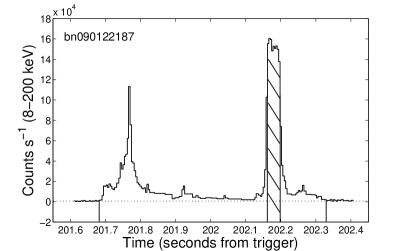
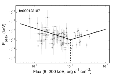
Figure 1.— Upper panel. Example of a Fermi-GBM bright burst (untriggered) from SGR J1550-5418. Each data bin is fit with either a COMPT or a 2BB model. The shaded region represents saturated intervals, which were not included in our analysis. The dotted line represents the background. Lower panel. COMPT $E_{\rm peak}$ as a function of flux for the same burst. The solid line is the best fit BPL model. The dashed line indicates where the break occurs in flux space, i.e., $F\approx 10^{-5}$ erg s^-1 cm^-2. The two PL indices are $-0.12$ and $0.11$, for the parts below and above the break, respectively.

The time-integrated spectroscopy of SGR J1550-5418 bursts (von Kienlin et al. 2012, V12, Collazzi et al. in prep) has shown that their spectra are well fit by a Comptonized model (COMPT). The other model to best fit the data is a combination of two blackbody (BB) functions (2BB model), except for the bursts in October 2008. During that time frame, however, there were no bursts that met our fluence and flux selection criteria, therefore we were able to use COMPT and 2BB models in our time-resolved spectroscopy. In this section we discuss the analysis with both spectral models separately. For the spectral analysis we have used the software package RMFIT (v4.3), and we generated the detector response matrices with GBMRSP v1.81. Given the low number of counts per time bin we have minimized the Castor C-statistic to obtain the best spectral fit.

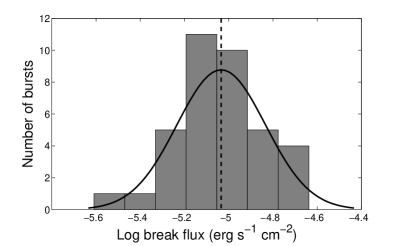
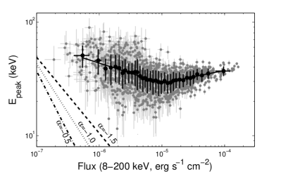
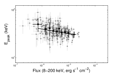
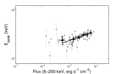
Figure 2.— Upper-left panel. Distribution of the break flux values in the $E_{\rm peak}$ evolution as a function of flux for the 37 bursts in our sample showing a break in the correlation between these two parameters. The solid and dashed lines are the best fit Gaussian model to the distribution and its respective mean. Upper-right Panel. $E_{\rm peak}$ evolution as a function of the 8-200 keV flux for all 49 bursts in our sample. Each dark-grey point is the result of a COMPT fit to a burst bin. The black dots represent the flux-binned data with 40 individual data points per bin. The black solid line is the best fit BPL model to the binned data. The dahsed, dotted, and dashed-dotted lines delimit the flux$-$$E_{\rm peak}$ parameter space, for index values of -1.5, -1.0, and -0.5, respectively. Lower-left panel. $E_{\rm peak}$ evolution as a function of the 8-200 keV flux for the 7 bursts with not enough data points above the flux break value. Lower-right panel. $E_{\rm peak}$ evolution as a function of the 8-200 keV flux for the 5 bursts with not enough data points below the flux break value. See text for more details.

3.1. Comptonized model

We started by fitting the COMPT model to all selected 4 ms time bins of each burst. The fit parameters of some time bins within the bursts were not well constrained due to a low number of counts. In such cases we binned the data with a coarser time resolution to accomplish a minimum constraint of 3$\sigma$ on $E_{\rm peak}$, the peak energy of the COMPT spectrum. As a result, 14 bursts have less than 5 time bins for spectral fitting, and we removed these bursts from our sample. Our final sample for spectral analysis with the COMPT model is, therefore, 49 bursts with a total number of 1393 time bins, for which we studied the correlations of the COMPT model parameters ($E_{\rm peak}$ and power-law index) with the 8$-$200 keV flux.

We first studied the spectral evolution with flux of each burst separately, plotting $E_{\rm peak}$ as a function of flux. To identify the trend of the evolution, we fit this correlation with a PL and a broken PL (BPL) model. The choice for a BPL model is based on the time-integrated spectroscopy results of SGR J1550-5418 (V12), and time-resolved spectroscopy of SGR J0501+4516 (Lin et al. 2011) which indicated a more complex relation between $E_{\rm peak}$ and flux than a PL (e.g., see Figure 1). An F-test showed an improvement in the fit, with a $>$99.99% non-chance occurrence, for 19 out of the 49 bursts. A more relaxed F-test criterion of $>$95% results in 37 out of the 49 bursts being better represented by a BPL than a PL (see e.g., Figure 1). Interestingly, the flux values at which the break occurs for these 37 bursts seem to cluster around a common value and does not depend on any of the burst parameters, e.g., $T_{\rm 90}$, average flux, etc. A Gaussian fit to the distribution of these break flux-values results in $F\approx(1.0\pm 0.2)\times 10^{-5}$ erg s^-1 cm^-2 (Figure 2, upper-left panel).

For the remaining 12 bursts, a single PL model was a better fit to the $E_{\rm peak}$ versus flux evolution. However, examining these bursts closely, we noticed that none of them had more than 5 data points above (7 out of 12) or below (5 out of 12) the break flux level of the majority of events. Figure 2 displays these single PL trends of the 7 and 5 events in the lower-left and lower-right panels, respectively. It is unclear whether these events would have followed the same break trend described above, had they had more intense or faint data points, respectively. Finally, we studied the correlation between $E_{\rm peak}$ and flux for all 49 bursts simultaneously, and we show this result as dark-grey points in the upper-right panel of Figure 2. Here we binned the data in flux requiring 40 individual data points in each bin, with the last bin (at the highest fluxes) having a slightly lower number of points. Each black dot in Figure 2 represents the weighted averages (in flux and $E_{\rm peak}$) of these 40 individual measurments, while the error bars correspond to their 1$\sigma$ deviations. Although not shown here, we also binned the data sorted by $E_{\rm peak}$, and tried different number of data points per bin (from 20 to 60), and we obtained consistent results. A BPL fit to the binned data is preferred at the $>99.99\%$ level over a single PL model. The BPL fit has a low-flux PL index of $-0.18\pm 0.02$ and a high-flux PL index of $0.12\pm 0.02$, with the break between the two PL regimes at a flux of $(9.1\pm 0.7)\times 10^{-6}$ erg s^-1 cm^-2 (8$-$200 keV) and a break $E_{\rm peak}$ of $32\pm 2$ keV, consistent with the 37-burst only fit. Finally, our PL indices and the break flux and $E_{\rm peak}$ values are similar to the values found in the time-integrated spectroscopy of SGR J1550-5418 bursts, and also in the time-resolved spectroscopy of SGR J0501+4516 bursts (Lin et al. 2011). These results are further discussed in Section 4.

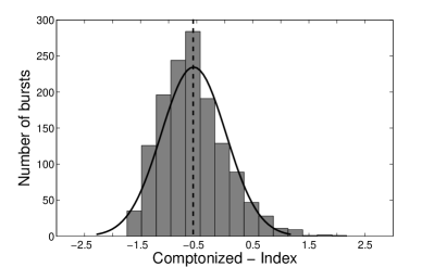
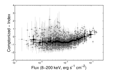
Figure 3.— Upper panel. COMPT index distribution from our time-resolved analysis. The solid line is a Gaussian fit to the data and the dashed line represents the mean of the Gaussian $\approx-0.5$. Lower Panel. COMPT index as a function of flux. Above the flux value of $10^{-5}$ erg s^-1 cm^-2 the index positively correlates with flux, whereas below, it remains constant around $-0.8$.

We find a more complicated correlation with flux than a single PL also for the COMPT PL index. V12 have shown that the index of the COMPT model in time-integrated spectroscopy is distributed narrowly around $-1$. Therefore, the OTTB model was an equally good fit to their time-integrated spectra, since it is similar to a COMPT model with an index of $-1$. We show in the top panel of Figure 3 the distribution of the index for our time-resolved analysis. The distribution is broader than for the V12 time-integrated study and the peak has now shifted to a higher value of $-0.55\pm 0.58$. To understand what prompted this shift, we plot in the bottom panel of Figure 3 the index as a function of flux. Below the flux value of $\sim 10^{-5}$ erg s^-1 cm^-2, identified as the break point in the $E_{\rm peak}$$-$flux correlation, the index appears constant with flux, with a value around $\sim-0.8$. It is only above the break where the indices become gradually steeper, following the same trend observed between the $E_{\rm peak}$ and flux values. We also note that, fitting some of the time-bins with the highest fluxes with the OTTB model, results in a bad fit, as one would expect if the index were deviating significantly from $-1$.

3.2. Two blackbody (2BB) function

We fit the initially selected 63 bursts (see Section 2) with a 2BB model, using our 4 ms time-bins. We binned parts of the light curves for significance, i.e., to different time resolutions to accomplish a $3\sigma$ constraint on the low and high BB temperatures. Since the 2BB model has more free parameters than the COMPT one, coarser time bins were required. Again, we removed bursts from the initial sample with less than 5 time bins after re-binning, resulting in 48 bursts and 994 individual time bins.

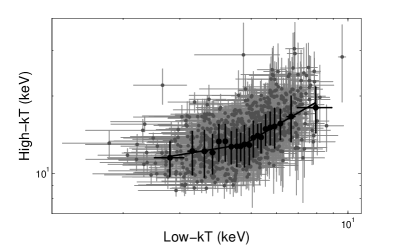
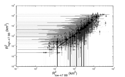
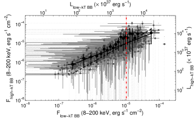
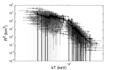
Figure 4.— Upper-left panel. High$-kT$ versus low$-kT$ BB temperature. The solid line is a BPL fit to the data with a break at $\sim$4.8 keV. Upper-right panel. Positive correlation between the radii of the emitting areas for the low- and high$-kT$ BB. Lower-left panel. Positive correlation between the fluxes (and luminosities assuming a distance of 5 kpc) of the low- and high$-kT$ BB. The dashed line represents a 1 to 1 relation. The dotted-dashed line is the $3\times 10^{40}$ erg s^-1 limit. Lower-right panel. Radius of emitting area as a function of temperature for the low- and high$-kT$ BB simultaneously. The low- and high$-kT$ BB are clearly separated in the plot, with the area of the high$-kT$ BB decreasing at a faster pace compared to the area of the low$-kT$ BB, as a function of temperature. In all four panels, dark-grey dots represent individual measurements with grey crosses as their error bars; the light-grey dotted lines represent the errors of data points with uncertainty in the flux and/or area larger than its measurement value. Black dots are binned data with 50 points per bin. The black solid lines are the best fit PL or BPL model to the binned data.

We examined several correlations between the fit parameters of the 2BB model, i.e., (1) temperatures of the low temperature (low$-kT$) BB versus high temperature (high$-kT$) BB; (2) the individual fluxes of the 2 BBs; (3) the emitting areas corresponding to the low$-kT$ and high$-kT$ BBs; (4) the radii of the emitting areas versus temperature for both BBs simultaneously. The effective radii of the emitting regions were calculated as in Lin et al. (2011), $R^{2}=(FD^{2}/\sigma T^{4})$ km², where $F$ is the flux in erg s^-1 cm^-2, $D$ is the distance to the source in km (here assumed as 5 kpc, Gelfand & Gaensler 2007; Tiengo et al. 2010), $\sigma$ is the Stefan-Boltzmann constant, and $T$ is the temperature in Kelvin. We used the same approach as for the COMPT model parameters to identify the trends of these different correlations, fitting them for each burst separately to a PL and a BPL model, and performing F-tests to evaluate the improvement in the fits.

For 26 of the 48 bursts, we find that the temperatures of the low$-kT$ BB versus high$-kT$ BB are best fit with a BPL ($>$95% probability for an improvement from a PL fit to occur by chance) with indices and breaks consistent with each other. The rest of the bursts follow similar but not statistically significant trends, due to low number of data points. Figure 4, upper-left panel, shows the relation between low$-kT$ and high$-kT$ values for all 48 bursts simultaneously. Here (and in all panels of Figure 4), we binned the data at 50 points per bin (black dots). We find that a BPL is a better fit to the data (black-solid line) compared to a single PL, at the $>99.99\%$ confidence level. Above the break, the relation is much steeper than below the break with slopes of $0.7\pm 0.2$ and $0.2\pm 0.1$, respectively. The corresponding break is at ($4.8\pm 0.3,13.1\pm 0.4$) keV. These results are different than the time-integrated spectroscopy of these bursts, which showed only a positive correlation between the low- and high$-kT$s, with a very weak hint for a possible break at low temperatures (V12); in that work, the slope of the single PL fit was much steeper, i.e., $1.86\pm 0.09$.

To rule out any systematic effect as the origin of the break, and in particular the fact that the temperature of the low$-kT$ BB falls below the Fermi/GBM energy coverage, we looked at Lin et al. (2012), who studied the combined spectra of the SGR J1550-5418 bursts simultaneously seen with Swift/XRT and GBM, thus extending the energy coverage down to 1 keV (see also Section 3.3). The authors found that the low- and high$-kT$ temperatures derived solely with GBM are equal to the ones derived from the joint XRT/GBM fits. The only deviations ($<1\sigma$) between the two results are noticeable at very low temperatures (below 4.8 keV for the low$-kT$), where the GBM-only fits gave slightly (but consistently) higher low$-kT$ temperatures than the joint ones. Therefore, if the break we see in our relation is due to systematic effects, one would also expect another break below a certain low$-kT$, where the relation becomes steeper.

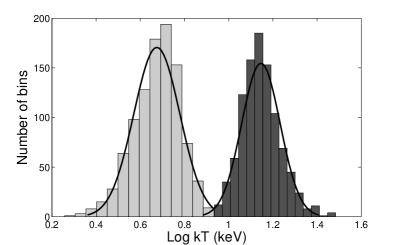
Figure 5.— Distributions of the low- and high$-kT$ BB temperatures with their respective best fit Gaussian models (solid lines).

The areas of the emitting regions as well as the fluxes of the low- and high$-kT$ BBs are positively correlated, with consistent single PL slopes for all 48 bursts in our sample. These correlations are shown at the upper-right and lower-left panels of Figure 4 (the areas are represented as $R^{2}$, with $R$ the radius). The PL slope of the correlation between the areas is $1.2\pm 0.3$, while for the fluxes it is $0.7\pm 0.1$. These slopes are consistent with the slopes for the time-integrated analysis of SGR J1550-5418 GBM bursts, which were $1.34\pm 0.04$ and $0.83\pm 0.02$, respectively. The slope of the correlation between the low- and high$-kT$ BB fluxes is close to the 1 to 1 relation (dashed line), indicating that the BBs contribute almost equally to the total burst flux. We note that in the case of time-resolved spectral analysis of SGR J0501+4516 bursts this slope is $1.1\pm 0.1$ (Lin et al. 2011), while for SGR 1900+14 it is $0.70\pm 0.03$ (Israel et al. 2008).

Besides comparisons between the two BB components, we investigated the relation between the emission area and temperature, for both the low- and high$-kT$ BB simultaneously. Most of the bursts showed a similar trend between these two parameters, namely that the area of the low$-kT$ BB decreases with temperature at a different pace than the area of the high$-kT$ BB. This same trend is seen when combining all the individual time bins, as shown in the lower-right panel of Figure 4. A BPL fit to the binned data has slopes of $-1.0\pm 0.3$ and $-6.4\pm 0.5$ for the low$-kT$ and high$-kT$ correlations, respectively and a break at a temperature of $\sim 7.9$ keV.

To determine the significance of this last relation, we calculated the Spearman rank correlation coefficients of the low- and high$-kT$ BB areas versus their corresponding temperatures. We found a correlation coefficient $r\approx-0.7$ and a probability of $\sim 99.9\%$ that the low$-kT$ area is correlated to the temperature, while for the high$-kT$ BB we found a stronger correlation $r\approx-1.0$ and a probability $>99.99\%$. The time-integrated spectroscopy of the SGR J1550-5418 bursts (V12) hint at a similar relation for the high$-kT$ BB, however, the low$-kT$ BB did not show any correlation between area and temperature.

Finally, we investigated the evolution of temperature and area with flux, $F$. The upper-left panel of Figure 6 (here we binned the data at 40 points per bin, i.e., black dots) shows the relation between the low- and high$-kT$ areas (corresponding to the high- and low$-kT$ BB temperatures) and fluxes. We again fit these correlations with a PL and a BPL to look for any possible breaks. It is clear that the area of both the low and high temperature BB increases with increasing flux. There is, however, a tendency for the low$-kT$ area to flatten at the highest fluxes, while the high$-kT$ area increases steadily. Indeed, the low$-kT$ area as a function of flux is best fit with a BPL with slopes of $1.3\pm 0.2$ and $0.5\pm 0.1$, respectively, and a break at $F=(3\pm 1)\times 10^{-6}$ erg s^-1 cm^-2, whereas the high$-kT$ area is best fit with a single PL with a slope of $1.3\pm 0.1$. A Spearman rank test shows that the correlation coefficients and probabilities for the low- and high$-kT$ areas as a function of flux are $r=0.8$, $p>99.99\%$ and $r=0.7$, $p>99.99\%$, respectively. We estimate that about $92\%$ of the low$-kT$-area data points with $F>10^{-4.5}$ erg s^-1 cm^-2 land at $\lesssim 10^{3}$ km², which corresponds to the 1$\sigma$ limit of the highest-flux binned data point.

The temperatures of the 2 BBs follow opposite trends with respect to flux, as can be seen in the upper-right panel of Figure 6. The low$-kT$ appears to positively correlate with flux, only above a break limit. This relation is best fit with a BPL, with slopes of $0.0\pm 0.1$ and $0.13\pm 0.02$, below and above $F=4\pm 2)\times 10^{-6}$ erg s^-1 cm^-2. The high$-kT$, on the other hand, shows a mild negative correlation with flux, and it is best fit with a single PL with a slope of $-0.04\pm 0.02$. The Spearman-rank correlation coefficients and probabilities are $r=0.5$, $p>99.99\%$, and $r=-0.3$, $p>99.99\%$, for the low- and high$-kT$ as a function of flux, respectively.

Given the correlations between the area and temperature with flux, next we examined the effect of the flux on the relation between area and $kT$. We created a color-coded plot by flux of these two parameters, which is shown in the lower-left panel of Figure 6. We note that the relation between area and $kT$ remains the same across all flux values, decreasing more steeply for the high temperatures compared to low temperatures. We show that also by separating our data into four flux ranges ($F<10^{-5.5}$, $10^{-5.5}<F<10^{-5.0}$, $10^{-5.0}<F<10^{-4.5}$ and $F>10^{-4.5}$), and fitting a PL and a BPL to the data in each flux range separately (Figure 6, lower-right panel; flux groups have been shifted for clarity). For the three highest flux ranges we find that a BPL is preferred over a PL fit at the $>99.99\%$ level, while for $F<10^{-5.5}$ a BPL is only required by the data at the $90\%$ level. Table 1 shows all fit results.

Table 1Area ($R^{2}$) versus $kT$ fit parameters for the different flux groups in the bottom-right panel of Figure 6.

Flux range	Slope below $kT_{\rm break}$	Slope above $kT_{\rm break}$	$kT_{\rm break}$
erg s-1 cm-2			keV
$F>10^{-4.5}$	$-2.2\pm 0.3$	$-5.3\pm 0.4$	$9\pm 1$
$10^{-5.0}<F<10^{-4.5}$	$-2.8\pm 0.3$	$-4.6\pm 0.4$	$7\pm 1$
$10^{-5.5}<F<10^{-5.0}$	$-3.0\pm 0.3$	$-4.4\pm 0.5$	$7\pm 1$
$F<10^{-5.5}$	$-3.8\pm 0.4$∗

• ^(∗) A single PL fit to the data.
  

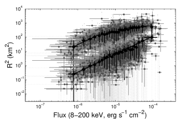
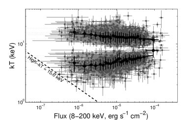
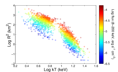
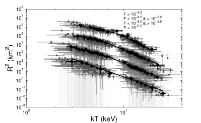
Figure 6.— Upper-left panel. Low- and high$-kT$ BB areas as a function of flux. Upper-right panel. Low- and high$-kT$ BB temperatures as a function of flux. The dashed line delimit the flux$-$low-kT parameter space for a high-kT value of 15 keV. Lower-left panel. Flux color-coded plot of the area as a function of temperature. Lower-right panel. Area as a function of temperature grouped in flux intervals from top to bottom as indicated by the legend. Flux groups are shifted arbitrarily for clarity. See text for details.

3.3. Simulations

We performed simulations with RMFIT (rmfit4.3) to determine the parameter space for the COMPT and 2BB models, for a typical magnetar burst spectrum detected with GBM.

We first checked whether we can recover the different spectral parameters we get from the real data through simulations of a large set of synthetic spectra. We chose three bursts with at least 10 bins at low fluxes ($<5\times 10^{-6}$ erg s^-1 cm^-2). We then generated 1,000 synthetic spectra for each bin and each relevant detector. Each synthetic spectrum was based on the sum of the predicted source counts and the measured background counts in each energy channel. The former counts were computed from the analytical function used to fit the real data (COMPT or 2BB) folded with the instrumental response function of the relevant detector. The background counts were estimated for each detector from the real data. Next, we applied Poisson fluctuations to the summed counts to obtain the final synthetic spectrum (see also, V12 and Guiriec et al. 2011). The resulting synthetic spectra were fitted with the model used to generate them. All input spectral parameters of both models were well recovered in these fits by comparing them and their statistical errors to the simulated parameter distributions and their uncertainties.

Next, we generated 1000 synthetic spectra using random input spectral parameters for the COMPT and 2BB models, decreasing the 8-200 keV flux from $4\times 10^{-6}$ erg s^-1 cm^-2 down to $10^{-7}$ erg s^-1 cm^-2, in steps of 0.2 dex. We then checked if the input spectral parameters were recovered within 1$\sigma$ , at the $90\%$ confidence level.

For the COMPT model, we varied the index between three different values ($\alpha=-0.5,-1.0,-1.5$), in order to have a better handle on $E_{\rm peak}$. The COMPT parameter space is shown in the upper-right panel of Figure 2, for all three values of the index; for each value, the area below the line cannot be retrieved with the instrumental sensitivity of GBM. It is clear from the simulations that even with a soft spectrum ($\alpha=-1.5$), we should have been able to detect bursts with $E_{\rm peak}$ as low as 10 keV for a 8-200 keV flux of $\sim 10^{-6}$ erg s^-1 cm^-2. The flux level goes down to $3\times\sim 10^{-7}$ erg s^-1 cm^-2 for a burst with a hard spectrum, $\alpha=-0.5$. Hence, we can conclude that the break we see in the $E_{\rm peak}-$flux (and $\alpha-$flux) relation at $\sim 10^{-5}$ erg s^-1 cm^-2 is not due to any systematic effects. We note that a very soft burst with $\alpha=-2.0$, would have been detected down to a $E_{peak}\approx 16$ keV, had it had a flux of $\sim 10^{-6}$ erg s^-1 cm^-2.

For the 2BB model, and similar to COMPT, we varied high-kT in a pre-defined set of values of 10, 15, and 20 keV, in order to have a good handle over the low-kT spectral parameters, which are harder to determine with GBM. We made sure to vary the normalizations of the two components in a way that both BBs contribute equally to the total flux, according to the well established relation between the low- and high-kT fluxes (Figure 4, Israel et al. 2008). We first found that the temperature of the high-kT component has little effect on the constraint of the low-kT spectral parameters. In the upper-right panel of Figure 6, we show the parameter space of the low-kT temperature with total flux. The parameter space in case of the 2BB model is smaller than in the case of COMPT, which is expected considering the extra free parameter. Nonetheless, according to our simulations, we should have been able to detect bursts with temperatures falling in the area of the extrapolation of the low-kT relation with flux seen above the break, hence concluding that the break we see in the $kT-$flux relation is real, and not due to systematic effects.

4. Discussion

4.1. Comparison to previous results

A large number of bursts were emitted by SGR J1550-5418 during the 2008-2009 active episode, especially on 2009 January 22 when the source emitted hundreds of bursts in nearly 24 hours. These bursts were detected by a multitude of high-energy space instruments. Savchenko et al. (2010, see also ) analyzed about 100 bursts detected on 2009 January 22 with the INTEGRAL SPI$-$ACS and ISGRI detectors. Scholz & Kaspi (2011) presented a detailed time-averaged spectral study of hundreds of bursts from SGR J1550-5418 detected with Swift/XRT. Finally, Enoto et al. (2012) studied 13 very weak bursts detected with Suzaku from SGR J1550-5418 ($F\lesssim 10^{-8}$ erg cm^-2). The better energy coverage and sensitivity of Fermi/GBM compared to these instruments allowed for a more detailed time-averaged spectroscopy of hundreds of bursts from SGR J1550-5418 (V12, see also von Kienlin et al. 2012). A COMPT model and a 2BB model were used to fit the time-integrated spectra, and V12 looked for correlations between the different fit parameters. For the COMPT model, V12 found a hint for a weak double correlation between $E_{\rm peak}$ and flux as opposed to the strong one we find here (Figure 2). This could be attributed to the fact that only very few bursts showed an average flux above the flux break-limit that we establish here (i.e., $F\sim 10^{-5}$ erg s^-1 cm^-2). On the other hand, for the 2BB model, V12 found a strong positive correlation between the low$-kT$ fluence and high$-kT$ fluence with a slope of 0.83, and between the low$-kT$ area and the high$-kT$ area with a slope of 1.34. These results are in perfect agreement with the results we derive for our time-resolved spectroscopy (Figure 4, but with fluxes instead of fluences). However, the area$-kT$ relation is clearer in our analysis than in V12, where we show that the low$-kT$ area decreases with temperature, only at a slower pace than the high$-kT$ area. This could be due to a combination of better statistics (more data) when performing time-resolved spectroscopy and/or the fact that the relation might be smeared out when performing time-integrated spectroscopy. Lin et al. (2012) studied the bursts of SGR J1550-5418 seen simultaneously with Swift/XRT and GBM, hence, broadening the energy coverage down to $\sim 1$ keV. Interestingly, fitting the time-integrated spectra of these bursts with the 2BB model, Lin et al. (2012) recovered, although at a much lower significance (most likely due to much lower statistics), the trend we see here between the areas and temperatures of the 2 BBs (Figure 4, lower-right panel). We also note that the values of our fit parameters are comparable to results derived from time-integrated spectroscopy of the bursts of other sources, e.g., SGR $1900+14$, SGR $1806-20$, and SGR J$0501+4516$ (Feroci et al. 2004; Nakagawa et al. 2007; Lin et al. 2011).

Detailed time-resolved spectroscopy on a large number of bursts with good statistics have been performed for SGR $1900+14$ (Israel et al. 2008), and SGR J$0501+4516$ (Lin et al. 2011). Israel et al. (2008) have studied the 2006 March 29 burst forest emitted by SGR $1900+14$, when more than 40 bursts were detected by Swift/BAT, 7 of which were intermediate flares (see also Olive et al. 2004; Lenters et al. 2003; Ibrahim et al. 2001). The authors found that a 2BB or a COMPT model explains the spectra best. For the 2BB model, they found average temperatures of $4.8\pm 0.3$ and $9.0\pm 0.3$ keV, and radii of $30\pm 2$ and $5.7\pm 0.5$ km, for the low- and high$-kT$ BB respectively. The average temperatures and radii for SGR J1550-5418 that we find are similar within $\sim 2\sigma$ uncertainties, $<$low$-kT>=4.8\pm 0.7$ keV, $<$high$-kT>=14\pm 2$ keV, and $<R_{\rm low-kT}>=20\pm 4$ km, $<R_{\rm high-kT}>=3.0\pm 1.0$ km.

However, the correlations between the 2BB-model parameters that Israel et al. (2008) found for SGR $1900+14$ differ slightly from the one we find here for SGR J1550-5418. For instance, Israel et al. (2008) found that the low- and high$-kT$ luminosities contributed almost similarly to the total energy up to a luminosity of $\sim 3\times 10^{40}$ erg s^-1, above which the low$-kT$ luminosity appears to saturate, and the high$-kT$ luminosity increases steadily to $\sim 3\times 10^{41}$ erg s^-1. We do not see a similar effect for SGR J1550-5418 in the lower-right panel of Figure 4, where the luminosities of the low- and high$-kT$ components are positively correlated up to $\sim 3\times 10^{41}$ erg s^-1, an order of magnitude higher than the $\sim 3\times 10^{40}$ erg s^-1 limit (red dotted-dashed line) derived with Israel et al. (2008).

Finally, the $R^{2}-kT$ correlation that Israel et al. (2008) found is similar to the one we find here but only for their brightest events with luminosities $>3\times 10^{40}$ erg s^-1, where the area of the low$-kT$ decreases with temperature, at a slower pace than the area of the high$-kT$ component. Below this luminosity, the relation for both the low- and high$-kT$ areas changes sharply. Although we see a change in the area$-kT$ correlation with flux for SGR J1550-5418 (Figure 6, lower panels), it is more gradual than the sharp turnover that Israel et al. (2008) reports for SGR $1900+14$.

Lin et al. (2011) studied the time-resolved spectra of the five brightest Fermi/GBM bursts emitted by SGR J$0501+4516$, fitting them with a COMPT model and a 2 BB model. The authors found a clear double correlation between $E_{\rm peak}$ and flux with a break at a flux value of $\sim 10^{-5}$ erg s^-1 cm^-2. Although this value is consistent with the one we derive for SGR J1550-5418 (Figure 2), this could be a pure coincidence, considering the difference in distance between the two sources (2 and 5 kpc for SGR J$0501+4516$ and SGR J1550-5418 respectively). Moreover, the slopes of the BPL of the $E_{\rm peak}$-flux relation for SGR J$0501+4516$ are in agreement, within uncertainties, to the values we report here for SGR J1550-5418 (Section 3.1). For the 2BB model, Lin et al. (2011) found (similar to Israel et al. 2008 and our results) that the high$-kT$ area decreases faster than the low$-kT$ area as a function of temperature. The authors did not find a correlation between $kT$ or area and flux, although, the quality of the data was not constraining.

Finally, we note that the large amount and superb quality of data that we have in hand helped reveal new trends between the fit parameters of the COMPT and, especially, the 2BB model, showing the spectral evolution during short bursts with unprecedented detail. For the COMPT model, we established for the first time a strong positive correlation between the index and flux, above the break flux-value of $\sim 10^{-5}$ erg cm^-2 s^-1; the exact value of the $E_{\rm peak}$-flux relation turnover. Noteworthy new trends for the 2BB model are, (1) the increase in area with flux, accompanied with a decrease in temperature, for the high$-kT$ component, (2) the increase in low$-kT$ area with flux while $kT$ remains constant, until they reach a common break point in flux where the area starts to saturate and $kT$ starts increasing, and (3) the smooth change in the slopes of the BPL fit to the area$-kT$ relation, and disappearing at the lowest fluxes where a PL is sufficient to explain the area$-kT$ relation, with a slope of $\sim-4$. We discuss the physical interpretation of these new results in the context of the magnetar model in the next section.

4.2. Radiative mechanism of SGR J1550-5418 bursts

In the following subsections, we interpret our results in the context of the magnetar model. We would like to note first that the similarity in the evolution of the 2BB and COMPT model parameters with flux for all SGR J1550-5418 bursts indicates that they were all triggered, more or less, by the same mechanism. Moreover, all the correlations that we find here do not seem to depend on the intrinsic parameters of a given burst, i.e., independent of the average flux, $T_{90}$, fluence, etc., implying that the radiative region is developing, and subsequently cooling, in similar fashion during all bursts.

4.2.1 Two black body model

There are several models that describe the triggering mechanism of magnetar short bursts, most famously, the model of Thompson & Duncan (1995, TD95 hereafter, see also ). TD95 considered the possibility that departure from magnetostatic equilibrium in the internal magnetic field of a magnetar, due for instance to Hall drift and ambipolar diffusion, will cause a build up of crustal stresses. These stresses, with the presence of the ultra-strong magnetic field, will result in the cracking of the crust, and the injection of an Alfven wave into the magnetosphere. Energetic particles are accelerated throughout the region of the Alfven wave, creating a trapped fireball of photon-pair plasma in the magnetosphere. Another model for triggering SGR bursts involves a magnetospheric reconnection caused by magnetic instability in the magnetosphere (Lyutikov 2003; Gill & Heyl 2010). This model can lead to the formation of a plasma fireball trapped inside magnetospheric flux lines (Gill & Heyl 2010), and also to thermal emission from heating of the magnetar surface. We note that the crust cracking model can lead to significant magnetospheric reconnection, since the external magnetic field will feel any instability in the internal one.

Regardless of the triggering mechanism, the trapped fireball formed during SGR bursts is hot, $T\gtrsim 50~{}$keV, with an extremely high density (TD95). Hence, the radiative mechanism of short SGR bursts is the cooling of a hot, optically thick plasma, confined by an ultra-strong magnetic field (B$>$B_QED). In this regime, the dominant energy exchange process is Compton scattering, and due to the high optical depth in the fireball, photons will most likely be thermalized. The diffusion time-scale across the fireball at a distance $R$ from the NS surface is much larger ($\sim 10^{4}$ s, TD95) than the typical SGR burst time-scale ($\sim 0.2$ s) due to the enormous optical depth through the pair plasma. Hence, the fireball likely loses energy as its cool surface layer propagates inwards (TD95). A gradient in the magnetic field is expected throughout the fireball due to its large coronal volume ($B\propto R^{-(2+p)}$, $0<p<1$ depending on the twist of the external dipole field, and $R$ is the distance from the NS surface, Thompson et al. 2002), causing a gradient in the effective temperature of the fireball at different heights above the NS surface (TD95). The true spectrum would then be a distorted multi-color BB.

Alternatively, Israel et al. (2008, see also ) attributed the 2BB model, which they used to fit the SGR $1900+14$ bursts, to the effect of the strong magnetic field ($B>B_{\rm QED}$) on the scattering cross-sections of the two polarization states of the photons (Herold 1979; Meszaros et al. 1980). In super-strong magnetic fields, E-mode photons (photons with electric vector perpendicular to B) have a much reduced cross-section and can potentially diffuse out from deep inside the magnetosphere very close to the NS surface, equivalent to the high$-kT$ component. O-mode photons, on the other hand, have a much higher cross-section and diffuse out from further out in the magnetosphere at large radii, correpsonding to the low$-kT$ component (TD95, Lyubarsky 2002). However, van Putten et al. (2013), modeling hydrostatic atmospheres in super-strong magnetic fields, showed that the E- and O-mode photospheres are very close in both temperature ($\Delta kT_{\rm E-O}\sim 1$ keV) and location, in sharp contrast to our findings (and those of Israel et al. 2008) between the low- and high$-kT$ components. We note that the true picture is even more complicated due to the fact that the evolving fireball during a given burst will sample a large range of field strengths and orientations, thereby mixing the radiative transfer elements of Compton opacity.

One way of overcoming the complications mentioned above, is if the 2BB components represent two physically, and geographically distinct emitting regions, each with their own E-mode and O-mode photospheres. According to the distribution of areas and temperatures of our 2BB modeling, one would expect a hot one located close to the NS surface (or a hot spot on the surface), and a cooler one located further out in the magnetosphere. The large spatial separation between the two emitting areas ($\sim$2 orders of magnitude in $R^{2}$) will most likely induce a profound difference in magnetic field morphology between these two zones. Nonetheless, the strong positive correlations that we find between the areas and fluxes of these two regions indicate that they are very strongly connected, and emitting at similar rates.

How do these two emitting regions evolve during a burst? For the high$-kT$ emitting region, the decrease in temperature (although small) and increase in area with flux (Figure 6, upper-panels, which is also true within each burst) is a clear indication of an adiabatically expanding emitting region, in line with the fireball model. The area of this emitting region ranges from a small hot spot on the NS surface ($\sim 0.2$ km) up to a radius of $\sim 5$ km. This radius is consistent with the size of the effective radiative zone of the footpoints of the plasma fireball according to TD95 (considered to be the E-mode photosphere), which is about $R_{\rm NS}/2$. Also, the temperature of this emitting region varies slightly, ranging on average from 10 keV to 15 keV (Figures 5 and 6), although fluxes vary by more than 3 orders of magnitude. This is also in line with the cooling fireball model, which predicts a slight spectral variation of the emergent spectrum from the emitting region (TD95).

The evolution of the low$-kT$ component with flux is not straightforward to interpret. The temperature of this emitting region appears constant at very low fluxes while the area increases at a similar rate as the high$-kT$ area (i.e., with the same slope of $\sim 1$, Figure 6, upper-panels). At $F\approx 10^{-5.5}$ erg s^-1 cm^-2, the area starts to saturate while the temperature starts increasing. Since both BB components emit radiation at the same rate (Figure 4, lower-left panel), an increase in temperature for the low$-kT$ component with increasing flux, while its area starts saturating, is inevitable in order to maintain the same energy density as the high$-kT$ component.

At the highest fluxes, the radius of the low$-kT$ emitting area seems to reach a maximum of $R_{\rm max}\sim 30$ km (see Section 3.2, and upper-left panel of Figure 6). This radius is much bigger than the NS radius (assuming surface emission), even if we include the effect of gravitational lensing, $R_{\rm app}=R(1-2GM/Rc^{2})^{-1/2}$, where $R_{\rm app}$ is the apparent radius of the NS at infinity, $R$ and $M$ are its radius and mass (Pechenick et al. 1983; Psaltis et al. 2000; Özel 2013). In fact, considering even the largest and most massive neutron stars allowed by theoretical equation of states (Lattimer & Prakash 2001), we have $R_{\rm app}\approx 20$ km (Figure 3 in Lattimer 2012), much lower than the saturation radius of the low$-kT$ emitting region. On the other hand, in the context of the fireball model, where the surface area $A_{\rm max}=\pi R_{\rm max}^{2}$ is a closed magnetospheric magnetic field bundle that anchors the emitting plasma, the saturation at such a level is expected since, for obvious geometrical reasons, it is difficult for the emitting region to be significantly larger than the NS area.

In the crust-cracking model for triggering SGR bursts (TD95), this saturation radius, $R_{\rm max}\sim 30$ km, of the high$-kT$ component has very important consequences. The frequency of the Alfven wave responsible for the creation of the photon-pair plasma fireball is, $\nu_{\rm max}=c/R_{\rm max}\approx 10^{4}$ Hz (which is consistent with a characteristic seismic mode frequency for neutron star crusts; Blaes et al. 1989). This harmonic excitation of the magnetosphere, like any other, has a minimum characteristic excitation radius, $R_{\nu}$ (TD95). This excitation radius cannot exceed the radius of the magnetic loop, $R_{\rm Loop}$, trapping the plasma fireball, $R_{\nu}<R_{\rm Loop}$, as this will result in an inefficient excitation (TD95).

The maximum effective area of the low$-kT$ component, $\pi R_{\rm max}^{2}$, could be assumed to be a fraction, $l_{5}/R_{*}$, of the expected projected area of the relevant magnetic field loop, $\pi R_{\rm Loop}^{2}$, where $l=l_{5}\times 10^{5}$ cm is the length-scale of the surface crack (TD95), and $R_{*}$ is the NS radius (assumed to be 10 km). This implies that

$$R_{\rm Loop}\sim(R_{*}/l_{5})^{1/2}R_{\rm max}\sim 100~{}{\rm km,}$$ (1)

assuming $R_{\rm max}=30$ km. This $l_{5}/R_{*}$ scaling comes from the fact that the derived radius, $R_{\rm max}$, of the low$-kT$ effective area spans magnetic field lines anchored over a large angle of order unity on the stellar surface, whereas in the case of a magnetic loop with small area footpoints (corresponding to the hot BB effective area), a smaller angle of order $\sim l_{5}/R_{*}$ is expected. Finally, according to the star-quake model, the minimum excitation radius of the Alfven wave is (TD95),

$$R_{\nu}\sim 10~{}B_{15}^{-2}\left(\frac{\theta_{\rm max}}{10^{-3}}\right)\left(\frac{V_{\mu}}{1.4\times 10^{8}{\rm~{}cm~{}s^{-1}}}\right)^{-1}~{}l_{5}~{}{\rm km},$$ (2)

where $B=B_{15}\times 10^{15}$ G is the core magnetic field strength, $\theta_{\rm max}\sim 10^{-3}-2\times 10^{-1}$ is the yield strain of the crust (Horowitz & Kadau 2009), and $V_{\mu}\sim(0.4-1.4)\times 10^{8}$ cm s^-1 is the shear wave velocity (Steiner & Watts 2009; Douchin & Haensel 2001). As mentioned above, since $R_{\nu}<R_{\rm Loop}\sim 100$ km, this yields a crustal internal magnetic field,

$$\begin{split}B&\gtrsim 3.2\times 10^{14}\left(\frac{R_{\rm Loop}}{100{\rm~{}km}}\right)^{-1/2}\left(\frac{\theta_{\rm max}}{10^{-3}}\right)^{1/2}\\ &\left(\frac{V_{\mu}}{1.4\times 10^{8}{\rm~{}cm~{}s^{-1}}}\right)^{-1/2}l_{5}^{1/2}~{}{\rm G}.\end{split}$$ (3)

We note that we used the limits on $V_{\mu}$ and $\theta_{\rm max}$ that yield the stringent lower limit on the crustal internal magnetic field $B$. A more reasonable values for $V_{\mu}$ ($=0.7\times 10^{8}$ cm s^-1, Steiner & Watts 2009), and $\theta_{\rm max}$ ($=0.1$, Horowitz & Kadau 2009), and substituting $R_{\rm Loop}$ with $R_{\rm max}$ results in,

$$\begin{split}B&\gtrsim 4.5\times 10^{15}\left(\frac{R_{\rm max}}{30{\rm~{}km}}\right)^{-1/2}\left(\frac{\theta_{\rm max}}{0.1}\right)^{1/2}\\ &\left(\frac{V_{\mu}}{0.8\times 10^{8}{\rm~{}cm~{}s^{-1}}}\right)^{-1/2}l_{5}^{1/2}~{}{\rm G}.\end{split}$$ (4)

We could also derive an upper-limit on the crustal internal magnetic field considering that the maximum observed energy, $E_{\rm max}=L_{\rm max}\times 4_{\rm ms}\sim 1.2\times 10^{39}$ erg, where $4_{\rm ms}$ is the bin time-interval, does not exceed the maximum magnetic energy possibly released in an area $l_{5}^{2}$ on the crust, which is $E_{\rm max}\sim 4\times 10^{40}~{}l_{5}^{2}~{}B_{15}^{-2}~{}(\theta_{\rm max}/10^{-3})^{2}$ erg (TD95). Taking $\theta_{\rm max}=0.1$, the above implies,

$$B\lesssim 5.8\times 10^{17}\left(\frac{\theta_{\rm max}}{0.1}\right)l_{5}~{}{\rm G}.$$ (5)

Another interesting finding in our analysis is the $R^{2}-kT$ relation, and its dependence on flux, which is once again a complicated result to interpret qualitatively (Figure 6, lower-panels). For instance, at the lowest fluxes ($F<10^{-5.5}$ erg s^-1 cm^-2) we find that $R^{2}\propto kT^{-3.8\pm 0.4}$, i.e., following lines of constant luminosities ($F\propto R^{2}kT^{4}$). The relation breaks from the above with increasing flux. This indicates that at the lowest fluxes, photons emitted by both components follow a perfect Planckian distribution, and starts deviating from it with increasing flux. One possible way to achieve a purely thermal spectrum is if photon splitting (Adler et al. 1970; Baring 1995; Baring & Harding 2001; Usov 2002; Chistyakov et al. 2012) is the dominant source of photon number changing (TD95). At the lowest fluxes, the size of the high$-kT$ component is extremely small (some tens of meters), and very likely most of the emitted radiation is in the form of E-mode photons. At such small distance from the NS, the magnetic field is super-critical, and due to the high temperature of the high$-kT$ component at these lowest fluxes, photon splitting is very efficient (low$-kT\sim 14$ keV$>kT_{\rm sp}\sim 11$ keV, where $kT_{\rm sp}$ is the BB temperature at which the photon splitting rate is sufficient to maintain LTE, TD95), leading to complete thermalization of the high$-kT$ component. With increasing flux, the high$-kT$ temperature starts dropping and the spectrum starts deviating from a pure Planckian, perhaps due to other radiative processes coming into play, e.g., double Compton scattering ($e+\gamma\rightarrow e+\gamma+\gamma$) and Bremsstrahlung. For the low$-kT$ component, the picture is not clear, mostly due to the variation in field morphology and opacity for both scattering and photon splitting at high altitudes. However, since these two components appear to be strongly coupled (Figure 4), we speculate that a deviation in the high$-kT$ photon distribution from a pure Planckian model would lead to the deviation in the low$-kT$ component as well.

4.2.2 Comptonized model

The COMPT model that we use here in our time-resolved spectroscopy is meant to mimic classical problems of unsaturated Comptonization (see Lin et al. 2011 for more details). In this model, photons scatter repeatedly inside a corona of hot electrons, until they reach the plasma temperature, $E\sim kT_{\rm e}$. Further heating is impossible and a spectral turnover ($E_{\rm peak}$) emerges. The power-law index below the turnover ($\lambda$) depends on the mean energy gain per collision and the probability of photon loss from the bubble (Rybicki & Lightman 1979). Hence, the index $\lambda$ depends only on the magnetic Compton$-y$ parameter ($y_{\rm B}$), $\lambda=1/2-\sqrt{9/4+4/y_{\rm B}}$, with $y_{\rm B}=4kT_{\rm e}/(m_{\rm e}c^{2}){\rm max}\{\tau_{\rm B},\tau_{\rm B}^{2}\}$. Here $\tau_{\rm B}$ is the effective optical depth inside the scattering medium, modified by the strong magnetic field, and ${\rm max}\{\tau_{\rm B},\tau_{\rm B}^{2}\}$ is the mean number of scatterings per photon.

We note that in magnetars, such a corona of hot electrons could develop in the inner magnetosphere, caused by the twisting of the external magnetic field lines (Beloborodov & Thompson 2007; Thompson et al. 2002; Thompson & Beloborodov 2005; Nobili et al. 2008). The magnetic reconnection model of Lyutikov (2003) for triggering SGR bursts fits this picture well, with any reconnection event being accompanied with magnetic field line twists.

The correlation that we find between the index $\lambda$ and flux is interesting in the context of the COMPT model (Figure 3). At low fluxes, $F\lesssim 10^{-5}$ erg s^-1 cm^-2, $\lambda$ is distributed around $\sim-1$, i.e., the flattest possible spectra. Such spectra are achieved through repeated Compton upscattering with $y_{\rm B}>>1$. However, with increasing fluxes, $\lambda$ starts increasing to reach $\sim 1$ at the highest fluxes. Compton upscattering of soft photons has difficulty generating such spectra. These high values for $y_{\rm B}$ suggest high opacity, and strong thermalization might be taking place inside the corona. Moreover, the $E_{\rm peak}$-flux relation enforces this conclusion. The anti-correlation that we see between these two parameters below the break at $F\approx 10^{-5}$ erg s^-1 cm^-2 (Figure 2, which roughly corresponds to the break we see in the $R^{2}-$flux and $kT-$flux relations for the low$-kT$ component) could be explained if there were coronal radius expansion (exactly the case of the high$-kT$ BB component, see above). On the other hand, the switch in this relation above the break and the hardening of the spectra with flux, indicates a saturation radius of the coronal volume, again corresponding to the saturation radius that we see for the low$-kT$ component. In the light of the above results, there is no reason not to prefer a true thermal spectrum at all fluxes for SGR J1550-5418 bursts, i.e., throughout the evolution of a given burst. Similar results were derived by Lin et al. (2012) when studying the broadband, 1$-$200 keV, time-integrated spectra of SGR J1550-5418 bursts.

5. Concluding remarks

In this paper, we have shown the importance of high time-resolution in the study of the spectral evolution of SGR bursts. We were able to put to test the emission from a hot, optically thick, fireball of photon-pair plasma, predicted to form during SGR short bursts, according to a number of models for triggering magnetar flares (TD95, Gill & Heyl 2010, Heyl & Hernquist 2005). We were able to follow the evolution of the emitting plasma in an unprecedented detail. Nonetheless, the very detailed observational picture presented in this paper motivates a more in depth modeling of the development and evolution of scattering/splitting cascades involving photon-pair fireballs in magnetar magnetospheres, taking into account the many physical and geometrical effects, to better understand the emission mechanism taking place during magnetar bursts.

References

- Adler et al. (1970) Adler, S. L., Bahcall, J. N., Callan, C. G., & Rosenbluth, M. N. 1970, Physical Review Letters, 25, 1061
- Aptekar et al. (2001) Aptekar, R. L., Frederiks, D. D., Golenetskii, S. V., et al. 2001, ApJS, 137, 227
- Baring (1995) Baring, M. G. 1995, ApJ, 440, L69
- Baring & Harding (2001) Baring, M. G. & Harding, A. K. 2001, ApJ, 547, 929
- Beloborodov & Thompson (2007) Beloborodov, A. M. & Thompson, C. 2007, ApJ, 657, 967
- Blaes et al. (1989) Blaes, O., Blandford, R., Goldreich, P., & Madau, P. 1989, ApJ, 343, 839
- Camilo et al. (2007) Camilo, F., Ransom, S. M., Halpern, J. P., & Reynolds, J. 2007, ApJ, 666, L93
- Chistyakov et al. (2012) Chistyakov, M. V., Rumyantsev, D. A., & Stus’, N. S. 2012, Phys. Rev. D, 86, 043007
- Douchin & Haensel (2001) Douchin, F. & Haensel, P. 2001, A&A, 380, 151
- Duncan & Thompson (1992) Duncan, R. C. & Thompson, C. 1992, ApJ, 392, L9
- Enoto et al. (2012) Enoto, T., Nakagawa, Y. E., Sakamoto, T., & Makishima, K. 2012, MNRAS, 427, 2824
- Fenimore et al. (1994) Fenimore, E. E., Laros, J. G., & Ulmer, A. 1994, ApJ, 432, 742
- Feroci et al. (2004) Feroci, M., Caliandro, G. A., Massaro, E., Mereghetti, S., & Woods, P. M. 2004, ApJ, 612, 408
- Gavriil et al. (2002) Gavriil, F. P., Kaspi, V. M., & Woods, P. M. 2002, Nature, 419, 142
- Gelfand & Gaensler (2007) Gelfand, J. D. & Gaensler, B. M. 2007, ApJ, 667, 1111
- Gill & Heyl (2010) Gill, R. & Heyl, J. S. 2010, MNRAS, 407, 1926
- Göğüş et al. (1999) Göğüş , E., Woods, P. M., Kouveliotou, C., et al. 1999, ApJ, 526, L93
- Göğüş et al. (2000) Göğüş, E., Woods, P. M., Kouveliotou, C., et al. 2000, ApJ, 532, L121
- Guiriec et al. (2011) Guiriec, S., Connaughton, V., Briggs, M. S., et al. 2011, ApJ, 727, 33
- Halpern et al. (2008) Halpern, J. P., Gotthelf, E. V., Reynolds, J., Ransom, S. M., & Camilo, F. 2008, ApJ, 676, 1178
- Herold (1979) Herold, H. 1979, Phys. Rev. D, 19, 2868
- Heyl & Hernquist (2005) Heyl, J. S. & Hernquist, L. 2005, ApJ, 618, 463
- Horowitz & Kadau (2009) Horowitz, C. J. & Kadau, K. 2009, Physical Review Letters, 102, 191102
- Ibrahim et al. (2001) Ibrahim, A. I., Strohmayer, T. E., Woods, P. M., et al. 2001, ApJ, 558, 237
- Israel et al. (2010) Israel, G. L., Esposito, P., Rea, N., et al. 2010, MNRAS, 408, 1387
- Israel et al. (2008) Israel, G. L., Romano, P., Mangano, V., et al. 2008, ApJ, 685, 1114
- Kaneko et al. (2010) Kaneko, Y., Göğüş, E., Kouveliotou, C., et al. 2010, ApJ, 710, 1335
- Kouveliotou et al. (1998) Kouveliotou, C., Dieters, S., Strohmayer, T., et al. 1998, Nature, 393, 235
- Kouveliotou et al. (1993a) Kouveliotou, C., Fishman, G. J., Meegan, C. A., et al. 1993a, Nature, 362, 728
- Kouveliotou et al. (1993b) Kouveliotou, C., Meegan, C. A., Fishman, G. J., et al. 1993b, ApJ, 413, L101
- Kouveliotou et al. (1999) Kouveliotou, C., Strohmayer, T., Hurley, K., et al. 1999, ApJ, 510, L115
- Kouveliotou et al. (2001) Kouveliotou, C., Tennant, A., Woods, P. M., et al. 2001, ApJ, 558, L47
- Kumar et al. (2010) Kumar, H. S., Ibrahim, A. I., & Safi-Harb, S. 2010, ApJ, 716, 97
- Lattimer (2012) Lattimer, J. M. 2012, Annual Review of Nuclear and Particle Science, 62, 485
- Lattimer & Prakash (2001) Lattimer, J. M. & Prakash, M. 2001, ApJ, 550, 426
- Lenters et al. (2003) Lenters, G. T., Woods, P. M., Goupell, J. E., et al. 2003, ApJ, 587, 761
- Lin et al. (2012) Lin, L., Göğüş, E., Baring, M. G., et al. 2012, ApJ, 756, 54
- Lin et al. (2011) Lin, L., Kouveliotou, C., Baring, M. G., et al. 2011, ApJ, 739, 87
- Lyubarsky (2002) Lyubarsky, Y. E. 2002, MNRAS, 332, 199
- Lyutikov (2003) Lyutikov, M. 2003, MNRAS, 346, 540
- Meegan et al. (2009) Meegan, C., Lichti, G., Bhat, P. N., et al. 2009, ApJ, 702, 791
- Mereghetti et al. (2009) Mereghetti, S., Götz, D., Weidenspointner, G., et al. 2009, ApJ, 696, L74
- Mereghetti & Stella (1995) Mereghetti, S. & Stella, L. 1995, ApJ, 442, L17
- Meszaros et al. (1980) Meszaros, P., Nagel, W., & Ventura, J. 1980, ApJ, 238, 1066
- Nakagawa et al. (2007) Nakagawa, Y. E., Yoshida, A., Hurley, K., et al. 2007, PASJ, 59, 653
- Nobili et al. (2008) Nobili, L., Turolla, R., & Zane, S. 2008, MNRAS, 386, 1527
- Olive et al. (2004) Olive, J.-F., Hurley, K., Sakamoto, T., et al. 2004, ApJ, 616, 1148
- Özel (2013) Özel, F. 2013, Reports on Progress in Physics, 76, 016901
- Paczynski (1992) Paczynski, B. 1992, actaa, 42, 145
- Pechenick et al. (1983) Pechenick, K. R., Ftaclas, C., & Cohen, J. M. 1983, ApJ, 274, 846
- Perna & Pons (2011) Perna, R. & Pons, J. A. 2011, ApJ, 727, L51
- Psaltis et al. (2000) Psaltis, D., Özel, F., & DeDeo, S. 2000, ApJ, 544, 390
- Rea et al. (2013) Rea, N., Israel, G. L., Pons, J. A., et al. 2013, ArXiv e-prints
- Rybicki & Lightman (1979) Rybicki, G. B. & Lightman, A. P. 1979, Radiative processes in astrophysics
- Savchenko et al. (2010) Savchenko, V., Neronov, A., Beckmann, V., Produit, N., & Walter, R. 2010, A&A, 510, A77
- Scholz & Kaspi (2011) Scholz, P. & Kaspi, V. M. 2011, ApJ, 739, 94
- Steiner & Watts (2009) Steiner, A. W. & Watts, A. L. 2009, Physical Review Letters, 103, 181101
- Thompson & Beloborodov (2005) Thompson, C. & Beloborodov, A. M. 2005, ApJ, 634, 565
- Thompson & Duncan (1995) Thompson, C. & Duncan, R. C. 1995, MNRAS, 275, 255
- Thompson & Duncan (1996) Thompson, C. & Duncan, R. C. 1996, ApJ, 473, 322
- Thompson et al. (2002) Thompson, C., Lyutikov, M., & Kulkarni, S. R. 2002, ApJ, 574, 332
- Tiengo et al. (2010) Tiengo, A., Vianello, G., Esposito, P., et al. 2010, ApJ, 710, 227
- Usov (2002) Usov, V. V. 2002, ApJ, 572, L87
- van der Horst et al. (2012) van der Horst, A. J., Kouveliotou, C., Gorgone, N. M., et al. 2012, ApJ, 749, 122
- van Putten et al. (2013) van Putten, T., Watts, A. L., D’Angelo, C. R., Baring, M. G., & Kouveliotou, C. 2013, MNRAS
- von Kienlin et al. (2012) von Kienlin, A., Gruber, D., Kouveliotou, C., et al. 2012, ApJ, 755, 150
- Woods et al. (2005) Woods, P. M., Kouveliotou, C., Gavriil, F. P., et al. 2005, ApJ, 629, 985