Predicting missing links via significant paths

Abstract

Link prediction plays an important role in understanding the intrinsic evolving mechanisms of networks. With the belief that the likelihood of the existence of a link between two nodes is strongly related to their similarity, many methods have been proposed to calculate node similarity based on node attributes and/or topological structures. Among a large variety of methods that take into account paths connecting the target pair of nodes, most of them neglect the heterogeneity of those paths. Our hypothesis is that a path consisting of small-degree nodes provides a strong evidence of similarity between two ends, accordingly, we propose a so-called significant path index in this Letter to leverage intermediate nodes’ degrees in similarity calculation. Empirical experiments on twelve disparate real networks demonstrate that the proposed index outperforms the mainstream link prediction baselines.

PACS numbers

89.20.Ff, 89.75.Hc, 89.65.-s

I Introduction

Plenty of empirical and theoretical studies aim at understanding the intrinsics of evolving networks, from characterizing topological features to revealing network functions Albert and Barabási (2002); Dorogovtsev et al. (2002); Newman (2003); Boccaletti et al. (2006); Costa et al. (2007). Among fruitful research issues, link prediction is a fundamental challenge Lü and Zhou (2011); Getoor and Diehl (2005). Indeed, the extent to which the network evolution is explicable coincides with our capacity to predict missing links Wang et al. (2012); Zhang et al. (2013). In addition, the accurate predictions help recommend friends in online social networks Scellato et al. (2011); Wang et al. (2011), explore protein-to-protein interactions Mamitsuka (2012); Cannistraci et al. (2013), reconstruct airline networks Guimerà and Sales-Pardo (2009), boost e-commerce scales Huang et al. (2005); Lü et al. (2012), and so on.

Most conventional methods formalized the task of link prediction in the form of estimating the probability that two disconnected nodes would be linked, which was believed to be positively correlated with the similarity between them Lü and Zhou (2011); Liben-Nowell and Kleinberg (2007). Some researchers extracted node attributes and calculated node similarity in the Euclidean space of attributes, but unfortunately met the difficulty in extraction and sparsity  Yin et al. (2010); Schifanella et al. (2010). Instead, mainstream methods took into account topological similarity based on network structures only, and could be classified into three major classes Lü and Zhou (2011). The first class calculated topological similarity with global structural information, such as the Katz Index that counts all paths connecting two nodes with shorter paths preferred Katz (1953). Such global metrics showed fair performance in prediction but suffered from high computational complexity. The second class, defined on local structures, were much easier to calculate. Typical methods counted the number of common neighbors (CN) Newman (2001), usually with a penalization of large-degree end nodes (e.g., Salton Index Salton and McGill (1986), Sørensen Index Sørensen (1948), Hub Promoted Index Ravasz et al. (2002), Leicht-Holme-Newman Index Leicht et al. (2006), etc.), or of large-degree common neighbors, such as Adamic-Adar Index (AA) Adamic and Adar (2003) and Resource Allocation Index (RA) Zhou et al. (2009). Although successfully reducing the computational expense, local metrics suffered from relatively poor prediction performance. In order to find a nice tradeoff between performance and complexity, the third class of similarity metrics were proposed on quasi-local structures. The Local Path Index (LP) ignored long-path terms in Katz Index Zhou et al. (2009); Lü et al. (2009), and its bounded version (BLP) relates local paths in an elaborate way Papadimitriou et al. (2012). The Local Random Walk Index (LRW) limits a random walker within a local range Liu and Lü (2010), while the Superposed Random Walk Index (SRW) continuously released a random walker at the starting node to emphasize the nodes near the target node Liu and Lü (2010).

However, most existing methods simply summed paths up and neglected the heterogeneity in paths, i.e., the possibility that different paths, even with the same length, indicate different similarities between two end nodes. Take a problem in collaborative filtering Goldberg et al. (1992) for example. Since many people has read the popular series of Harry Potter, reading a Harry Potter book does not expose much information of a reader’s taste, and therefore finding neighbors for him is sometimes random. The overestimated similarity between such a reader and his dissimilar neighbors attributes to the user-book-user paths containing a large-degree node, the book of Harry Potter. Intuitively speaking, a path containing small-degree nodes indicates a greater similarity. An intermediate node with fewer neighbors is usually more selective in establishing links, and thus has greater similarity with each neighbor. Besides, its small degree sometimes implies a concentrated range of interests. Both reasons lead to a high probability that two of its neighbors are mutually similar. The case of a node with numerous neighbors is the opposite. It is not necessarily that two of its neighbors are mutually similar, e.g., it is probable that a reader with wide interests over various topics have two of his favorite books totally different. With that intuition we believe, two nodes with a small-degree common neighbor are more probable to be similar, which could be extended to a more general form that a path containing small-degree nodes provides an evidence of a greater similarity between two ends.

Inspired by the above discussion, we propose a new index to measure the contribution of a path when calculating the similarity between its two ends, namely the significant path index, or SP for short. The proposed index incorporates degrees of intermediate nodes into the path length, defining a path is significant if it is short and consists of small-degree intermediate nodes. Such a significant path is believed to reflect a great similarity between its two ends. Empirical results verify that the proposed index significantly improves prediction accuracy in link prediction, compared with five mainstream baselines.

II Problem and Metric

We here consider an undirected network $G(V,E)$, where $V$ and $E$ stand for the sets of nodes and links, respectively. To test the algorithm’s accuracy, the set of links, $E$, is randomly divided into two parts: the training set, $E^{T}$, is treated as known information, while the testing set (also called probe set or validation set in the literature), $E^{P}$, is used for testing and no information in this set is allowed to be used for prediction. Clearly, $E^{T}\bigcup E^{P}=E$ and $E^{T}\bigcap E^{P}=\emptyset$. Every link prediction algorithm aims at uncovering links in the testing set.

A standard metric, called the area under the receiver operating characteristic curve (AUC for short) Hanley and McNeil (1983) is used to quantify the prediction accuracy. Provided the rank of all non-observed links (i.e., links in $U-E^{T}$, where $U$ is the universal set) according to their estimated existent likelihoods, the AUC value can be interpreted as the probability that a randomly chosen link in $E^{P}$ (i.e., a link that indeed exists but does not belong to $E^{T}$ yet) is ranked higher than a randomly chosen link in $U-E$ (i.e., a non-existent link). If all the likelihood scores are generated from an independent and identical distribution, the AUC value should be about 0.5. Therefore, the degree to which the value exceeds 0.5 indicates how much better the algorithm performs than pure chance.

III Baselines

Under the simplest framework of link prediction Lü and Zhou (2011), each pair of nodes, $v_{x}$ and $v_{y}$, is assigned a similarity score $s_{xy}$. All non-observed links are ranked according to their scores, and the links with higher scores are supposed to be of higher existent likelihoods. Five mainstream algorithms (each corresponding to a similarity index) are implemented as baselines for performance comparison, described below.

Common Neighbors Index (CN) Newman (2001) measures the similarity between two nodes with the number of their common neighbors:

$$s^{CN}_{\mbox{\tiny xy}}=\left|\Gamma(x)\cap\Gamma(y)\right|,$$ (1)

where $\Gamma(x)$ denotes the set of neighbors of node $v_{x}$, and $\Gamma(x)\cap\Gamma(y)$ represents the set of common neighbors of node $v_{x}$ and $v_{y}$.

Adamic-Adar Index (AA) Adamic and Adar (2003) expands CN by emphasizing less-connected common neighbors, as:

$$s^{AA}_{\mbox{\tiny xy}}=\sum_{z\in\Gamma(x)\cap\Gamma(y)}\frac{1}{\log(k_{{}_{z}})}.$$ (2)

Resource-Allocation Index (RA) Zhou et al. (2009); Ou et al. (2007) simulates resource transmissions between two nodes, and penalizes common neighbors with large degrees, as:

$$s^{RA}_{\mbox{\tiny xy}}=\sum_{z\in\Gamma(x)\cap\Gamma(y)}\frac{1}{k_{{}_{z}}}.$$ (3)

Local Path Index (LP) Zhou et al. (2009); Lü et al. (2009) additionally counts the contribution of local paths with length three, as:

$$S^{LP}=A^{2}+\varepsilon A^{3},$$ (4)

where $A$ is the adjacency matrix and $\varepsilon$ is a free parameter.

Bounded Local Path Index (BLP) Papadimitriou et al. (2012) bounds local paths with structural coefficients according to path lengths:

$$s^{BLP}_{\tiny xy}=\sum_{i=2}^{l_{\max}}\frac{1}{i-1}\cdot\frac{\left|P_{i}(v_{x},v_{y})\right|}{\prod_{j=2}^{i}(N-j)},$$ (5)

where $l_{\max}$ indicates the maximum length under consideration, $P_{i}(v_{x},v_{y})$ is the set of all paths connecting $v_{x}$ and $v_{y}$ with length $i$, and $\left|P_{i}(v_{x},v_{y})\right|$ is the number of these paths.

IV Significant Paths

Our basic idea comes from the intuition that paths should not be counted indifferently: a short path consisting of small-degree intermediate nodes provides more evidence of a missing link connecting its two ends. In the proposed significant path index, we calculate the similarity between a pair of non-adjacent node by counting paths connecting them while penalizing both the lengths and the intermediate nodes’ degrees of those paths.

Definition 1

On an undirected unweighted network $G(V,E)$, the significance $\zeta$ of a path $q=\{v_{1},v_{2},\cdots,v_{n}\}$ equals to the sum of penalized degree of each intermediate node, as

$$\zeta(q)=\sum_{v_{i}\in M(q)}k_{i}^{\beta},$$ (6)

where $k_{i}$ is the degree of node $v_{i}$, $M(q)=\{v2_{,}\cdots,v_{n-1}\}$ is the set of intermediate nodes of path $q$, and $\beta$ is the degree-penalizing parameter that penalizes nodes with large degrees when $\beta<0$. This index has previously been applied to quantify the expected traffic congestion in transportation networks Yan et al. (2006).

Definition 2

On an undirected unweighted network $G(V,E)$, the significant path index $S_{xy}^{SP}$ of a pair of node $v_{x}$ and $v_{y}$ is the sum of significance of every path connecting $v_{x}$ and $v_{y}$, as:

$$S_{xy}^{SP}\propto\alpha_{1}\sum_{q\in P_{2}(v_{x},v_{y})}\zeta(q)+\alpha_{2}\sum_{q\in P_{3}(v_{x},v_{y})}\zeta(q)+\cdots,$$ (7)

where $\alpha_{\bullet}$ are the length-penalizing parameters that penalize paths with longer lengths and thus $\alpha_{l}>\alpha_{l^{\prime}}$ if $l<l^{\prime}$.

Since paths longer than three cost expensive computations but contribute little to predicting links Lü et al. (2009), we ignore those paths in practice. As only two length-penalizing parameters remain, we simply let $\alpha=\frac{\alpha_{2}}{\alpha_{1}}$ and rewrite Eq. (7) as follows:

$$\small S_{xy}^{SP}=\sum_{q\in P_{2}(v_{x},v_{y})}\sum_{v_{i}\in M(q)}k_{i}^{\beta}+\alpha\sum_{q\in P_{3}(v_{x},v_{y})}\sum_{v_{i}\in M(q)}k_{i}^{\beta}.$$ (8)

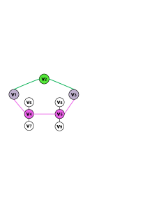
Figure 1: An example network to illustrate the significant path index.

The two parameters $\alpha$ and $\beta$ penalize path length and node degree respectively, capturing the intuition that the fewer nodes it passes through, the smaller degrees such nodes have, the stronger evidence the two ends of such path is actually connected by a missing link. Figure 1 shows a simple example to illustrate the significant path index. We calculate the SP index of node $v_{1}$ and $v_{3}$, and find a total of $2$ paths connecting them: $q_{1}=\{v_{1},v_{2},v_{3}\}$, $q_{2}=\{v_{1},v_{4},v_{5},v_{3}\}$. Comparing those two paths, $v_{2}$, the only intermediate node of $q_{1}$, appears more selective and is thus more similar with both $v_{1}$ and $v_{3}$, which suggests a larger probability that $v_{1}$ and $v_{3}$ are also similar to each other. In opposite, $q_{2}$ provides less evidence since $q_{2}$ is longer and its intermediate nodes have larger degrees.

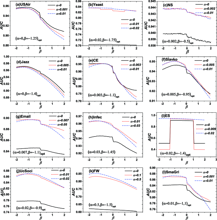
Figure 2: The prediction performance of SP index on twelve benchmark networks with different values of $\alpha$ and $\beta$ . For each network, the optimal values of $\alpha$ and $\beta$ are presented inside the corresponding plot. Notice that, for every case, the optimal $\beta$ is smaller than zero, indicating that to penalize the large-degree intermediate nodes.

V Data

Table 1: The basic topological features of the twelve benchmark networks. $\left|\textit{V}\right|$ denotes the number of nodes, $\left|\textit{E}\right|$ is the number of links, $\langle k\rangle$ represents the average degree, $\langle d\rangle$ denotes the average distance, $C$ indicates the clustering coefficient Watts and Strogatz (1998), $r$ indicates the assortativity coefficient Newman (2002), and $H$ is the degree heterogeneity, defined as $H=\frac{\langle k^{2}\rangle}{\langle k\rangle^{2}}$.

Nets	$\left|\textit{V}\right|$	$\left|\textit{E}\right|$	$\langle k\rangle$	$\langle d\rangle$	C	r	$H$
USAir	332	2128	12.81	2.74	0.749	-0.208	3.36
Yeast	2370	10904	9.2	5.16	0.378	0.469	3.35
NS	1461	2742	3.75	5.82	0.878	0.461	1.85
Jazz	198	2742	27.7	2.24	0.633	0.02	1.4
CE	453	2025	8.94	2.66	0.655	-0.225	4.49
Slavko	334	2218	13.28	3.05	0.488	0.247	1.62
Email	1133	5451	9.62	3.61	0.254	0.078	1.94
Infec	410	2765	13.49	3.63	0.467	0.226	1.39
ES	1272	6454	10.15	3.86	0.382	-0.012	2.46
UcSoci	1893	13825	14.62	3.06	0.138	-0.188	3.81
FW	128	2075	32.42	1.78	0.334	-0.112	1.24
SmaGri	1024	4916	9.6	2.98	0.349	-0.193	3.95

Experiments are performed on twelve real networks. We converted arcs into undirected links and removed loops and multi-links to make them simple networks, keeping their connectivity. (i) US Air97 (USAir) Batagelj and Mrvar (1998): the network of the US air transportation system. (ii) Yeast PPI (Yeast) Bu et al. (2003): the protein-protein interaction network of yeast. (iii) NetScience (NS) Newman (2006): the network of coauthorships between scientists publishing on the topic of networks. (iv) Jazz Gleiser and Danon (2003): the network of Jazz musicians. (v) C.elegans (CE) Watts and Strogatz (1998): the neural network of the nematode worm C.elegans. (vi) Slavko Blagus et al. (2012): the Facebook friendship network of Slavko $\check{Z}$itnik. (vii) Email network (Email) Guimera et al. (2003): the email communication network of University Rovira i Virgili (URV) in Tarragona, Spain. (viii) Infectious (Infec) Isella et al. (2011): the face-to-face contact network of people during the exhibition “Infectious: Stay Away” in 2009 at the Science Gallery in Dublin. (ix) EuroSiS web mapping study (ES) Van Welden (2004): mapping interactions between Science in Society actors on the Web of 12 European countries. (x) UC Irvine messages social network (UcSoci) Opsahl and Panzarasa (2009): the communication network according to the sent messages between users of an online community of students from the University of California, Irvine. (xi) Food Web of Florida ecosystem (FW) Bascompte (2004): the relationship of carbon exchanges in the cypress wetlands of South Florida during the wet season. (xii) Small & Griffith and Descendants (SmaGri) Hummon and Dereian (1989): the network composed of citations to Small & Griffith and Descendants. Table 1 reports the basic topological features of these networks.

Each original data set is randomly divided into a training set $E^{T}$ containing $80\%$ links, and a testing set $E^{P}$ containing $20\%$ links, while the connectivity in $E^{T}$ is guaranteed.

Table 2: Prediction accuracy measured by AUC values on the twelve benchmark networks. Each data point is an average over 10 independent realizations, each of which corresponds to a random 80%-20% division of training set and testing set. All the present results corresponding to the optimal cases by tuning the parameters if any. Numbers in brackets stand for the standard deviations.

AUC	CN	AA	RA	LP	BLP	SP
USAir	0.938(0.0064)	0.950(0.0072)	0.956(0.0075)	0.938(0.0073)	0.931(0.0100)	0.960(0.0132)
Yeast	0.703(0.0053)	0.705(0.0051)	0.705(0.0052)	0.780(0.0068)	0.836(0.0089)	0.847(0.0086)
NS	0.940(0.0114)	0.940(0.0114)	0.940(0.0114)	0.940(0.0118)	0.943(0.0095)	0.944(0.0094)
Jazz	0.954(0.0054)	0.961(0.0047)	0.970(0.0046)	0.954(0.0053)	0.951(0.0056)	0.972(0.0044)
CE	0.914(0.0119)	0.948(0.0102)	0.954(0.0101)	0.914(0.0112)	0.911(0.0076)	0.957(0.0089)
Slavko	0.941(0.0098)	0.945(0.0099)	0.946(0.0100)	0.944(0.0101)	0.943(0.0104)	0.951(0.0096)
Email	0.844(0.0071)	0.846(0.0071)	0.846(0.0070)	0.893(0.0064)	0.902(0.0054)	0.899(0.0077)
Infec	0.939(0.0096)	0.943(0.0094)	0.944(0.0093)	0.954(0.0124)	0.958(0.0065)	0.964(0.0062)
ES	0.910(0.0059)	0.912(0.0061)	0.912(0.0061)	0.936(0.0073)	0.938(0.0051)	0.945(0.0056)
UcSoci	0.773(0.0066)	0.778(0.0068)	0.778(0.0068)	0.838(0.0051)	0.870(0.0059)	0.871(0.0073)
FW	0.612(0.0162)	0.615(0.0158)	0.620(0.0146)	0.800(0.0121)	0.641(0.0051)	0.873(0.0142)
SmaGri	0.833(0.0074)	0.843(0.0073)	0.843(0.0076)	0.857(0.0079)	0.875(0.0076)	0.874(0.0103)

VI Results

We firstly report the performance of SP with $\beta$ varying in the range $[-2,2]$ and $\alpha$ from $0$ to $1.0$ as suggested in Lü et al. (2009), measured with average AUC under $10$ independent runs with different random divisions of training sets and testing set. As shown in Figure 2, the performance varies with $\beta$ continuously in most cases. For every data set, a single peak is observed when $\beta<0$. It demonstrates the intuition we claimed that the intermediate nodes with smaller degrees provide stronger evidence of the existence of a missing link than nodes with larger degrees. Specifically, in most data sets a sudden decrease around $\beta=0$ is observed, at which the index changes from penalizing paths consisting of large-degree intermediate nodes ($\beta<0$) to penalizing paths consisting of small-degree intermediate nodes ($\beta>0$). Since large-degree nodes usually lie in many paths (as suggested by the strong correlation between degree and betweenness, see for example Guimera et al. (2005)), in the case of $\beta>0$, many paths with large-degree nodes are wrongly assigned high contributions and thus a large proportion of nonexistent links will be put in the top positions, eventually leading to a large decline in algorithm’s performance.

The performance seems not sensitive to $\alpha$ as long as $\alpha>0$. In Figure 2, besides curves when $\alpha$ takes typical positive values such as $0.001$ and $0.01$, we intentionally provide the curve when $\alpha=0$, meaning deletion of long paths’ contributions. In most data sets, except for USAir and Jazz, there is a distinctive deviation between curves with $\alpha=0$ and $\alpha>0$. The AUC performance curve with $\alpha=0$ is obviously beneath the contrasts. Accordingly, SP is particularly useful for the networks with many long paths. The phenomenon indeed confirms that combination with long paths is very necessary.

To demonstrate the prediction ability, we report the performance of SP index with the optimal $(\alpha,\beta)$ value on $12$ data sets respectively. Table 2 reports the average AUC values of SP and baselines. SP achieves the best performance in $10$ out of $12$ data sets, and is the runner-up in the remaining two (see boldface in Table 2). Notice that those data sets represent different kinds of networks with heterogeneous topological features (see Table 1) and disparate organization principles, the comparison highlights that SP works well consistently on various situations.

Analyzing the difference in performance between SP and baselines, we realize that it is the penalization on large-degree nodes and consideration of long paths that explain the difference. CN indifferently counts the number of common neighbors on 2-hop paths, ignoring node degrees and long paths, resulting in its worst performance in most data sets. AA and RA extend CN by similarly penalizing large-degree nodes, and not surprisingly obtain better performance than CN. However, the fixed form of penalization limits their flexibility to adjust for disparate networks. Besides, ignoring long paths prevents them from better predictions in networks fulfilled with long paths such as Yeast. In contrast, LP and BLP take long paths into account and thus outperform on those two networks. However, lacking consideration of large-degree nodes, LP and BLP meets difficulty in accurately predict missing links in networks with plenty of large-degree nodes, such as USAir.

VII Conclusion and Discussion

We start from the intuition that a path containing small-degree nodes indicates a greater similarity, and thus provide more evidence of a missing link between its two ends. A Significant Path index (SP) is proposed to formalize that intuition into a similarity metric, summing up the discounted degrees of all intermediate nodes over all local paths connecting two non-adjacent nodes. Empirical results demonstrate that, with a negative parameter $\beta$ that penalizes large-degree nodes, the proposed SP outperforms five representative mainstream baselines, evaluated with AUC as binary classifiers. A sudden decrease in prediction performance is observed when $\beta$ changes from penalizing to encouraging large-degree nodes.

Looking at the parameters $\alpha$ and $\beta$, we find that instead of a fixed value of penalizing parameter, i.e., $\beta=-1$ in RA, the SP allows flexible value of penalizing parameter $\beta$, resulting in its performance among the best in most data sets. The contribution of long paths are weak but not negligible. In networks where long paths play a more important role, ignoring long paths is unwise and leads to poor performance, suggested by the performance of RA in Yeast, meanwhile an inappropriately large $\alpha$ also depresses the performance.

The SP starts a broad space for investigation on link prediction and facilitates new promising applications in the future, such as infrastructure constructions planning like traffic transportation, researches on the reactions between organisms in biological experiments, evolutions of people’s relations in social activities, controls of propagation of disease, protections of ecological system network, and so on.