Controlling Chimeras

Abstract

Coupled phase oscillators model a variety of dynamical phenomena in nature and technological applications. Non-local coupling gives rise to chimera states which are characterized by a distinct part of phase-synchronized oscillators while the remaining ones move incoherently. Here, we apply the idea of control to chimera states: using gradient dynamics to exploit drift of a chimera, it will attain any desired target position. Through control, chimera states become functionally relevant; for example, the controlled position of localized synchrony may encode information and perform computations. Since functional aspects are crucial in (neuro-)biology and technology, the localized synchronization of a chimera state becomes accessible to develop novel applications. Based on gradient dynamics, our control strategy applies to any suitable observable and can be generalized to arbitrary dimensions. Thus, the applicability of chimera control goes beyond chimera states in non-locally coupled systems.

1 Introduction

Collective behavior emerges in a broad range of oscillatory systems in nature and technological applications. Examples include flashing fireflies, superconducting Josephson junctions, oscillations in neural circuits and chemical reactions, and many others [1, 2]. Phase coupled oscillators serve as paradigmatic models to study the dynamics of such systems [3, 4, 5, 6]. Remarkably, localized synchronization—in contrast to global synchrony—may arise in non-locally coupled systems where the coupling depends on the spatial distance between two oscillators. Dynamical states consisting of locally phase-coherent and incoherent parts have been referred to as chimera states [7, 8], alluding to the fire-breathing Greek mythological creature composed of incongruous parts from different animals. Chimera states are relevant in a range of systems; they have been observed experimentally in mechanical, (electro-)chemical, and laser systems [9, 10, 11, 12], and related localized activity has been associated with neural dynamics [13, 14, 15, 16, 17, 18, 19, 20, 21, 22, 23, 24]. By definition, local synchrony is tied to a spatial position that may directly relate to function: in a neural network, for example, different neurons encode different information [25, 26, 27]. In non-locally coupled phase oscillator rings, the spatial position of partial synchrony not only depends strongly on the initial conditions [7], but it also is subject to pseudo-random (i.e., low number) fluctuations [28]. These fluctuations are particularly strong for persistent chimeras for just few oscillators [29] as in typical experimental setups. This naturally leads to the question whether it is possible to control a chimera state and keep at a desired spatial location.

In this article, we derive a control scheme to dynamically modulate the position of the coherent part of a chimera. To the best of our knowledge, this is the first application of noninvasive control to spatial properties of chimera states. Our control is based on gradient dynamics to optimize general location-dependent averages of dynamical states. Defined as the place where local synchronization is maximal, the spatial location of a chimera state is such a space-dependent average. As control of spatially localized patterns, chimera control relates—by definition—to both traditional control approaches [30, 31, 32] as well as other of localized patterns in, for example, chemical [33] or optical [34] systems. However, the aim of chimera control differs from these control approaches. First, chimera control preserves a chimera state as a whole as opposed to classical engineering control. More specifically, its goal is not to change the dynamics qualitatively, that is, for example, to restore a turbulent system to a periodic state, but rather to control space dependent averages. Second, chimera control is noninvasive as a result of the underlying gradient dynamics. That is, in contrast to some approaches to control the spatial position of localized patterns [34], the control strength vanishes upon convergence. Third, chimera control extends beyond the spatial continuum limit, where the dynamics of individual oscillators are negligible. It applies to systems of finite dimension, even down to just a handful of inhomogeneous oscillators. In contrast to continuous spatial systems, where static or periodic localized patterns [35, 36, 14, 37] may shift, chimeras in finite dimensions are localized chaotic states [38] (similar to localized turbulence in pipe flows [39, 40]) subject to strong low number fluctuations [28]. In summary, chimera control modulates the spatial location of a chimera noninvasively even in low-dimensional system and preserves its “internal” incoherent oscillatory dynamics.

We anticipate chimera control to have a broad impact across different fields. On the one hand, the control scheme may elucidate how position is maintained in (noisy and heterogeneous) real world systems where spatial localization of synchrony plays a functional role, such as neural systems. On the other hand, however, it is the first step towards actually employing chimera states as functional localized spatio-temporal patterns. In fact, instead of passively observing chimera states, the aim of control is to actively exploit chimeras for applications by making the spatial location accessible. Its location could encode information which allows, for example, control mediated computation. Despite the differences to chimera control, the control of dynamical states, such as chaos, has led to many intriguing applications in their own right [32, 41, 42, 43]. So in analogy to the Greek mythological creature one may ask: what would you be able to do if you could control a fire-breathing chimera?

2 Chimeras in Non-Locally Coupled Rings

Rings of non-locally coupled phase oscillators provide a well studied model in which chimera states may occur [8]. Let $\mathbf{S}:=\varmathbb{R}/\varmathbb{Z}$ be the unit interval with endpoints identified and let $\mathbf{T}:=\varmathbb{R}/2\pi\varmathbb{Z}$ denote the unit circle. Let $d$ be a distance function on $\mathbf{S}$, $h:\varmathbb{R}\to\varmathbb{R}$ be a positive function, and $\alpha\in\mathbf{T}$, $\omega\in\varmathbb{R}$ be parameters. The dynamics of the oscillator at position $x\in\mathbf{S}$ on the ring is given by

$$\partial_{t}\varphi(x,t)=\omega-\int_{0}^{1}h(d(x,y))\sin\!\left(\varphi(x,t)-\varphi(y,t)+\alpha\right)\mathrm{d}y.$$ (1)

The coupling kernel $h$ determines the interaction strength between two oscillators depending on their mutual distance. The system evolves on the torus $\mathbf{S}\times\mathbf{T}$ where $x\in\mathbf{S}$ is the spatial position of an oscillator on the ring and $\varphi(x,t)\in\mathbf{T}$ its phase at time $t$ on the torus.

Chimera states are characterized by a region of local phase coherence while the rest of the oscillators rotate incoherently. Let $\phi\in\Phi:=\left\{\phi:\mathbf{S}\to\mathbf{T}\right\}$ denote a configuration of phases on the ring. The local order parameter

$$Z(x,\phi)=\int_{0}^{1}h(d(x,y))\exp(i\phi(y))\mathrm{d}y$$ (2)

is an observable which encodes the local level of synchrony of $\phi$ at $x\in\mathbf{S}$. That is, its absolute value $R(x,\phi)=\left|Z(x,\phi)\right|$ is close to zero if the oscillators are locally spread out and attains its maximum if the phases are phase synchronized close to $x$. A chimera state is a solution $\varphi(x,t)$ of (1) which consists of locally synchronized and locally incoherent parts. The value of the local order parameter yields local properties of a chimera. The local order parameter obtains its maximum at the center of the phase synchronized region and its minimum at the center of the incoherent region; cf. Figure 1 for a finite dimensional approximation.

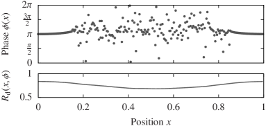
Figure 1: The local order parameter $R(x,\phi)$ encodes the spatial position of a chimera state in a ring of $N=256$ oscillators. Non-local coupling is given by the exponential kernel $h_{0}$; cf. (8). As a function of the oscillator phase $\phi(x)$ on the circle $\mathbf{S}$ (top panel), the maximum of $R$ indicates the center of the synchronized region, the minimum the position of the incoherent part (bottom panel).

3 Chimera Control

Is it possible to dynamically move a state to a desired position by exploiting drift properties? Before considering chimera states, we consider general solutions moving in space. Here we focus on systems with one spatial dimension but it is straightforward to extend the notions to higher dimensions. A solution of (1) may be seen as a one-parameter family of functions $\varphi_{t}\in\Phi$ which assign a phase to each spatial position. Let $Q:\mathbf{S}\times\Phi\to\varmathbb{R}^{n}$ be differentiable in the first argument. Think of $Q$ as an observable of the system which depends on the spatial position $\mathbf{S}$; here we look at the particular circular geometry because of its relevance in the context of chimera states on a ring, but one could as well consider observables on other geometries, such as the line $\varmathbb{R}$. A solution $\varphi_{t}$ of (1) with initial condition $\varphi_{0}\in\Phi$ is called $Q$-traveling along $\mathbf{S}$ if there are suitably smooth functions $y(t)$ and $q:\mathbf{S}\to\varmathbb{R}^{n}$ such that $Q(x,\varphi_{t})=q(x-y(t))$ for all $t$; in particular, a solution is $Q$-traveling at constant speed $v\in\varmathbb{R}$ along $\mathbf{S}$ if $Q(x,\varphi_{t})=q(x-vt)$ for all $t$. Hence, the temporal evolution of a $Q$-traveling solutions in terms of the observable $Q$ is a shift along $\mathbf{S}$.

If there is a way to influence the spatial motion in a controlled way, it can be used to optimize a general observable $Q$. Let $\partial_{z}f(z)|_{z_{0}}$ denote the partial derivative of a function $f$ with respect to $z$ at $z_{0}$, let $f^{\prime}$ denote its total derivative, and $\dot{z}$ the temporal derivative of a function $z(t)$. Let $\varphi_{t}$ be a $Q$-traveling solution with $q(x)$ and $y(t)$ such that $Q(x,\varphi_{t})=q(x-y(t))$. The function $y(t)$ describes the spatial position of $\varphi_{t}$ with respect to $Q$. For now, fix a target $x_{*}\in\mathbf{S}$ and assume that $q$ is differentiable with all critical points being extrema. The idea is to use an accessible system parameter that governs the evolution of $\varphi_{t}$ in terms of the observable $Q$ to maximize $Q$ at $x_{*}$, or, put differently, to use the knowledge how this accessible system parameter influences the evolution of $y(t)$ to maximize $q_{x_{*}}(y):=q(x_{*}-y)$ in $y$. To this end, we assume that for a given observable $Q$ there is a family $h_{a}$ of coupling kernels, indexed by ${a}\in A\subset\varmathbb{R}$, and a continuous invertible map $\nu:A\to\varmathbb{R}$ such that $\varphi_{t}$ is a $Q$-traveling solution at speed $\dot{y}=\nu({a})$ of (1) with coupling kernel $h_{a}$. In other words, we assume that the position $y(t)$ of the solution $\varphi_{t}$ is given by integrating $\nu({a})$. Of course, if ${a}$ is constant we have $Q(x,\varphi_{t})=q(x-\nu({a})t)$, i.e., $\varphi_{t}$ is $Q$-traveling at constant speed along $\mathbf{S}$.

Control can now be realized as gradient dynamics by choosing the parameter ${a}$ suitably. For $\gamma>0$ and assuming that the initial condition is not a local minimum, the function $q_{x_{*}}(y)$ is maximized if $y$ is subject to the gradient dynamics ${\dot{y}}=\gamma\partial_{y}q_{x_{*}}(y)$ since this choice implies that $\dot{q}_{x_{*}}\geq 0$. Note that $\partial_{y}q_{x_{*}}(y)=-q^{\prime}(x_{*}-y)=-\partial_{x}q(x-y)|_{x_{*}}$. Thus, if the function $y(t)$ of a $Q$-traveling solution $\varphi_{t}$ obeys

$${\dot{y}}=-\gamma\partial_{x}q(x-y)|_{x_{*}}=-\gamma\partial_{x}Q(x,\varphi_{t})|_{x_{*}},$$ (3)

then the function $Q(x,\varphi_{t})$ will attain a (local) maximum at $x=x_{*}$ in the limit of $t\to\infty$. At the same time, the map $\nu$ allows to use ${a}$ as a control parameter. By definition we have $\dot{y}(t)=\nu(a(t))$ and therefore (3) yields

$$a(t)=\nu^{-1}\left(-\gamma\partial_{x}Q(x,\varphi_{t})|_{x_{*}}\right),$$ (4)

a direct relationship between the traveling solution and the parameter ${a}$. More precisely, choosing a time dependent control parameter ${a}$ according to (4) yields a traveling solution whose dynamics maximize the observable $Q$ at $x_{*}$.

Note that convergence to the target through control does not depend on the function $\nu$. Moreover, the assumption that $\nu$ is invertible can be relaxed. If $\nu:A\to U$ be invertible where $U\subset\varmathbb{R}$ is an open interval that contains zero, then we can just extend $\nu^{-1}$ from $U$ onto the real line $\varmathbb{R}$ by choosing $\nu^{-1}(u)=\sup_{a\in A}\nu^{-1}(a)$ for $u\geq\sup U$ and $\nu^{-1}(u)=\inf_{a\in A}\nu^{-1}(a)$ for $u\leq\inf U$ or vice versa. Effectively this yields gradient dynamics ${\dot{y}}=\gamma(t)\partial_{y}q_{x_{*}}(y)$ with time-dependent parameter $0<\gamma(t)\leq\gamma$ which maximize $q_{x_{*}}$. Thus, with the assumptions on $\nu$ as above, control remains applicable. On the other hand, to determine the maximal convergence speed one has to to take other properties of $\nu$ into account.

The same gradient approach can be used to apply control to sufficiently smooth time-dependent control targets. Even though we have so far assumed $x_{*}$ to be constant, the control target can also be taken to be piecewise constant since the values at the discrete points of discontinuity do not change the integral. Therefore, control is suitable for any time dependent control target $x_{*}(t)$ that can be approximated by a piecewise constant functions. Of course, convergence to a time-dependent control target will only be approximate as control ensures that the maximum is attained only in the limit as $t\to\infty$.

To control chimeras we apply this general control scheme to the absolute value $R$ of the local order parameter. Since it encodes the local level of synchrony, dynamics that maximize the local order parameter through $R$-traveling chimera solutions yield a chimera moving to a specified target position. Note that $R(x,\varphi_{t})=r(x)$ of a chimera state $\varphi_{t}$ is stationary [8, 44] so it is $R$-traveling at constant speed zero. Here we further assume that there is a family of coupling kernels $h_{a}$ that lead to $R$-traveling solutions at nonzero speed $\nu({a})$. The control parameter dynamics (4) for the observable $R$ are

$$a(t)=\nu^{-1}\left(-\gamma\partial_{x}R(x,\varphi_{t})|_{x_{*}}\right).$$ (5)

Hence, choosing a time dependent control parameter ${a}$ according to (5) is equivalent to gradient dynamics to maximize the local order parameter at $x_{*}$. For the original chimeras with a single coherent region [7, 8], i.e., where $R$ has a global maximum, the limiting position of a chimera subject to control is unique. For chimera states with multiple coherent regions [20, 44], the local order parameter will attain a local maximum at the target position.

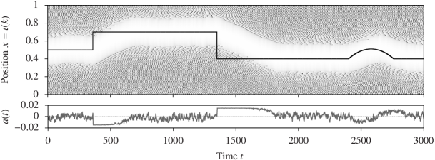
Figure 2: The position of the chimera adjusts to the imposed target for the control scheme applied to a ring of $N=256$ oscillators. The top panels shows the phase evolution in the co-rotating frame defined by the phase in the synchronized region with maximal order parameter. The black line is the target position. The bottom panels depict the asymmetry parameter ${a}(t)$ bounded by ${a}_{\mathrm{max}}=0.015$, cf. (10). Once the target position is reached, ${a}$ stays close to zero.

4 Implementation in Finite Dimensional Rings

Most real world systems consist of a finite number of oscillators; we thus implement chimera control in an approximation of the continuous equations (1) by a system of $N$ phase oscillators. Let $\iota(k)=k/N$ be the position of the $k$th oscillator on the ring $\mathbf{S}$. Let $\omega_{k}\in\varmathbb{R}$ be the intrinsic frequency of each oscillator and initially we assume that the oscillator system is homogeneous, i.e., $\omega_{k}=\omega$ for all $k=1,\ldots,N$. The temporal evolution of each oscillator is given by

$$\dot{\varphi}_{k}=\omega_{k}-\frac{1}{N}\sum_{j=1}^{N}h(d(\iota(k),\iota(j)))\sin(\varphi_{k}-\varphi_{j}+\alpha)$$ (6)

for $k=1,\ldots,N$. Here, $d(x,y)=\big{(}\big{(}x-y+\frac{1}{2}\big{)}\operatorname{mod}1\big{)}-\frac{1}{2}$ is a signed distance function on $\mathbf{S}$. The local order parameter of the discretized system is defined for $\varphi=(\varphi_{1},\ldots,\varphi_{N})\in\mathbf{T}^{N}$ as

$${Z}_{\mathrm{d}}(x,\varphi)=\frac{1}{N}\sum_{j=1}^{N}h(d(x,\iota(j)))\exp(i\varphi_{j})$$ (7)

and its absolute value $R_{\mathrm{d}}(x,\varphi)$ encodes the local level of synchrony; cf. Figure 1.

To implement the chimera control scheme (4), the assumption of a monotonic relationship $\nu$ between a system parameter and the chimera’s drift speed has to be satisfied. Asymmetric coupling kernels may induce drift in dynamical systems on a continuum such as standard pattern forming systems [14, 45, 46]. We employ the recent observation that breaking the symmetry of the coupling kernel slightly also results in the drift of the chimeras in finite-dimensional systems [47]. The result is a monotonic relationship $\nu(a)$ between asymmetry and drift speed [47] independent of the system’s dimension. Here we consider a family of exponential coupling kernels

$$h_{a}(x)=\cases{\exp\left(-\kappa(1-{a})\left|x\right|\right)&{if } $x<0$\\ \exp\left(-\kappa(1+{a})\left|x\right|\right)&{if } $x\geq 0$.}$$ (8)

for ${a}\in(-1,1)$, where ${a}$ determines the symmetry of the coupling kernel. The coupling in (8) can be analytically related to oscillators coupled in reactive-diffusive media [48] subject to convective concentration gradients of the coupling medium. For sufficiently small $\left|a\right|\lessapprox 0.015$ the relationship $\nu$ between drift and asymmetry is approximately linear at ${a}=0$ and the resulting drifting chimeras are in good approximation $R$-traveling with constant speed. We use this single observation for the implementation of chimera control. Note the particular shape of $h_{a}$ is not crucial for control since other asymmetric coupling kernels also lead to drift. However, the topic of drifting chimera states in systems with asymmetric coupling kernels deserves a treatment in its own right, and we refer to a forthcoming article [47] for details.

The relationship between asymmetry parameter ${a}$ and the drift speed now allows for a straightforward implementation of the control scheme. The control rule (5) acts as feedback control through the asymmetry parameter. If the chimera is off target, the nonzero asymmetry yields a drift of the chimera towards the target according to the derivative of the local order parameter at the target position. Once the target is approached, the control subsequently reduces the asymmetry and acts a corrective term keeping the chimera on target. For the finite ring, a discrete derivative at $x_{*}\in\mathbf{S}$ can be defined for a given $\delta\in(0,0.5)$ by

$$\Delta^{\delta}_{x_{*}}R_{\mathrm{d}}(x,\varphi(t))=\frac{1}{2\delta}\left({R_{\mathrm{d}}(x_{*}+\delta,\varphi(t))}-{R_{\mathrm{d}}(x_{*}-\delta,\varphi(t))}\right).\$$ (9)

For small $\delta$ we have $\Delta^{\delta}_{x_{*}}R_{\mathrm{d}}(x,\varphi(t))\approx\partial_{x}R_{\mathrm{d}}(x,\varphi(t))|_{x_{*}}$. We employ the sigmoidal function $\lambda(x)=2(1+\exp(-x))^{-1}-1$ to ensure an upper bound ${a}_{\mathrm{max}}>0$ for the asymmetry parameter ${a}(t)$ to prevent chimeras from breaking down. Let $K>0$ be a constant. Given a target position $x_{*}\in\mathbf{S}$, an approximation of (5) for control is

$${a}(t)=a_{\mathrm{max}}\lambda\left(K\Delta^{\delta}_{x_{*}}R_{\mathrm{d}}(x,\varphi(t))\right).$$ (10)

where $K$ can be determined from the gradient control parameter $\gamma=K\nu^{\prime}(0)$. These dynamics will maximize the local order parameter at $x_{*}$. In other words, a chimera $\varphi(t)$ will move along the ring until its synchronized part is centered at $x_{*}$.

Solving the dynamical equations subject to control numerically shows that the chimera adjusts to the imposed target position. Figure 2 shows a simulation for $N=256$ phase oscillators with $K=100$, and a time dependent target position $x_{*}(t)$. The simulation is carried out with initial conditions as in [8] and an adaptive integration step to meet standard error tolerances. We discretized (10) in time by keeping the asymmetry parameter piecewise constant with an update every $\Delta t=1$ time units. The chimera tracks the changes of the target position and adjusts to match new control targets.

Effectively, the control can be seen as a coupling of the dynamical equations to a function of the local order parameter. In contrast to systems with symmetric order parameter-dependent interaction [49, 50], in chimera control the order parameter induces a time-dependent asymmetry (5) to the nonlocal coupling to realize directed motion [47]. As a result, the chimera drifts along a subspace defined by the symmetry of the uncontrolled system to achieve the target position.

5 Control of Fluctuations

An uncontrolled chimera will exhibit pseudo-random (low number) fluctuations [28] along the ring $\mathbf{S}$ which persist even when the symmetry of the system is broken. These fluctuations are particularly strong for small numbers of oscillators. Since chimera control acts as a feedback mechanism to correct deviations from the target position, it counteracts the fluctuations along the ring. Thus, the control scheme keeps a chimera localized at a target position even in low-dimension systems despite the strong spatial fluctuations for a small number of oscillators; cf. Figure 3 (top).

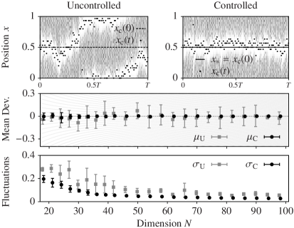
Figure 3: Top: Control successfully suppresses pseudo-random finite size fluctuations ($N=30$ oscillators) in low-dimensional rings. Center: The average deviation $\mu_{\mathrm{U}},\mu_{\mathrm{C}}$ of a chimera from its initial position (straight lines in top panel) over $T=3000$ time units is distributed around zero without control (gray) but on spot with control (black). Thin gray lines indicate a deviation of a single oscillator. Bottom: Control also reduces the fluctuations of the chimera due to pseudo-random movement significantly, even for very few oscillators ($N\leq 30$) as quantified by $\sigma_{\mathrm{U}},\sigma_{\mathrm{C}}$. Points are slightly set off horizontally for legibility.

To quantify how chimera control suppresses the pseudo-random fluctuations, we tracked the center of the coherent region $x_{\mathrm{c}}(t)\in\mathbf{S}$ in a homogeneous ring. More specifically, for a given initial condition $\varphi(0)$ for (6) with initial position $x_{\mathrm{c}}(0)$ we first solved the uncontrolled system numerically to obtain the mean $\mu_{\mathrm{U}}$ and standard deviation $\sigma_{\mathrm{U}}$ of $d(x_{\mathrm{c}}(0),x_{\mathrm{c}}(t))$ over $T$ time units. Similarly, one obtains $\mu_{\mathrm{C}}$ and $\sigma_{\mathrm{C}}$ for the controlled chimera with $x_{*}=x_{\mathrm{c}}(0)$ as the target position. Averages over multiple runs are shown in Figure 3. Applying control keeps the average position of the chimera on target for $N\geq 30$ (the standard deviation is below a single oscillator). Moreover, the fluctuations of the chimeras’ positions are greatly reduced for all $N$. Hence, control renders the spatial position of a chimera usable even when the number of oscillators is small.

6 Control for Inhomogeneous Rings

For control to be relevant in real-world applications, it has to be robust to inhomogeneities in the system. So far we have considered the case of homogeneous rings where all oscillators have the same intrinsic frequency $\omega_{k}=\omega$ for $k=1,\ldots,N$. In fact, when all oscillators are identical, the ring has a rotational symmetry where the symmetry group acts by translations along the ring. Control allows to shift a chimera along the orbit of the associated symmetry operation. Chimera states persist if the rotational symmetry is broken by choosing nonidentical frequencies, i.e. chimera solutions can be continued while adiabatically increasing heterogeneity [51]. Assume nonidentical intrinsic frequencies $\omega_{k}=1+\eta_{k}$ where $\eta_{k}$ are independently sampled from a normal distribution centered at zero with standard deviation $\sigma_{\omega}$. Chimeras can be observed for the inhomogeneous ring for $\sigma_{\omega}\lessapprox 0.03$ before the chimeras break down. In contrast to homogeneous oscillators, a chimera now has preferred positions on the inhomogeneous ring due to the lack of rotational symmetry which is determined by the actual value of the frequencies $\omega_{k}$.

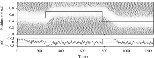
Figure 4: Control of chimera states is successful even in heterogeneous rings of $N=256$ oscillators, yielding qualitatively similar results as for homogeneous rings. As in Figure 2 the phase of the oscillators in the top panel is shown in a corotating frame. The standard deviation of the oscillators’ frequencies is $\sigma_{\omega}=0.01$. Note that control is robust to choosing larger bounds on the maximal control parameter ${a}_{\mathrm{max}}=0.05$ facilitating fast control and leading to faster convergence to the target position.

Remarkably, control remains applicable for inhomogeneous rings of oscillators with distributed frequencies $\omega_{k}$. Note that the control perturbations (4) are calculated from the averaged quantity $R_{\mathrm{d}}$. Thus, small fluctuations induced by inhomogeneities average out. The resulting controlled chimera follows the imposed target position even for comparatively large standard deviations of the frequency distribution; cf. Figure 4. The qualitative impact of control is the same as in homogeneous rings. However, if the maximal control parameter ${a}_{\mathrm{max}}$ is too small, even a controlled chimera may get “stuck” while moving towards the target position.

Larger bounds for the control parameter ${a}$ counteract this limitation induced by inhomogeneity. In fact, control is not only robust to choosing ${a}_{\mathrm{max}}>0.015$ but a sufficiently large value of ${a}_{\mathrm{max}}$ allows a chimera to be placed at an arbitrary position along any inhomogeneous ring. Moreover, the chimera attains its target position quickly. Carrying out the same statistics as previously (i.e., as for assessing the control of pseudo random fluctuations for homogeneous rings) reveals that for sufficiently large control parameters the chimera will stay on arbitrary targets (not shown). Hence, control renders the spatial position of a chimera usable in both homogeneous and inhomogeneous systems.

7 Functional Chimera States

Control is essential to give chimera states persistent functional meaning. Chimera states arise in real physical systems that are related to various technological applications. These include collections of mechanical, (electro-)chemical, and optical systems [9, 10, 11, 12]. Chimera control now allows to use the localized nature of a chimera state for arbitrary novel applications in these contexts. As simple example for a technological application of chimera states, one may envision a digital chimera computer where spatial location directly encodes information. Note that as long as the number of oscillators is large enough one is not limited to a digital computer with just two states but one could also consider an arbitrary number of states up to approximately encoding a continuous variable. Take two antipodal points $x^{0},x^{1}\in\mathbf{S}$ on the ring and say that the system is in state 0 if a chimera is centered at $x^{0}$ and in state 1 if it is centered at $x^{1}$; cf Figure 5(a). Thus, in this setup, the spatial position of a chimera encodes information. With active control this spatial encoding is reliable because there are no random flips between states 0 and 1. Note that only few oscillators are necessary to encode information because control reduces the pseudo-random fluctuations even in low-dimensional systems.

$\begin{array}[]{c}\includegraphics[scale={0.95}]{img/gChimeraCircleLblL}\end{array}:=0\hskip 31.2982pt\begin{array}[]{c}\includegraphics[scale={0.95}]{img/gChimeraCircleLblR}\end{array}:=1$

(a) Location Encodes Information

$\begin{array}[]{c}\includegraphics[scale={0.95}]{img/gChimeraCircleLblSyncA}\end{array}\begin{array}[]{c}\stackrel{{\scriptstyle[}}{{\textrm{}}}{coupling}]{x_{*}^{\mathbf{B}}\left(\varphi^{\mathbf{A}}(t)\right)}{\includegraphics[scale={0.31}]{img/sArrow}}\end{array}\begin{array}[]{c}\includegraphics[scale={0.95}]{img/gChimeraCircleLblSyncB}\end{array}$

(b) Assignment “$\mathbf{B}=\mathbf{A}$” (synchronization)

$\begin{array}[]{c}\includegraphics[scale={0.95}]{img/gChimeraCircleLblSyncA}\end{array}\begin{array}[]{c}\stackrel{{\scriptstyle[}}{{\textrm{}}}{coupling}]{x_{*}^{\mathbf{B}}\left(\varphi^{\mathbf{A}}(t)\right)}{\includegraphics[scale={0.31}]{img/sArrow}}\end{array}\begin{array}[]{c}\includegraphics[scale={0.95}]{img/gChimeraCircleLblNotB}\end{array}$

(c) NOT operation “$\mathbf{B}=\lnot\mathbf{A}$” (inversion)

Figure 5: In a digital chimera computer, control allows for the spatial position of a chimera to encode information. A chimera located at antipodal points $x^{0},x^{1}$ can for example encode bits (Panel (a)). Here the angle denotes the spatial coordinate on the ring $\mathbf{S}$ and the radius the current phase; one obtains the torus by identifying the two boundary components of the annulus. By coupling multiple rings through control (black arrows), one can now realize computations in a chimera computer. The current position of a chimera is given by $R_{\mathrm{max}}^{X}=\operatorname*{arg\,max}_{x\in\mathbf{S}}R_{\mathrm{d}}\big{(}x,\varphi^{X}(t)\big{)}$, $X\in\left\{{\mathbf{A}},{\mathbf{B}}\right\}$ (black triangles) and coupling between the rings (black arrows) is achieved by the dependence of the control target (red triangles) $x_{*}^{\mathbf{B}}$ of Ring $\mathbf{B}$ on the position $R_{\mathrm{max}}^{\mathbf{A}}$ of the chimera on Ring ${\mathbf{A}}$, cf. (11). Synchronization of position corresponds to copying bits (Panel (b)), inversion of the position to a NOT gate (Panel (c)).

Control also allows to change the value of the “bit” dynamically to perform computations. If we take two rings, Ring $\mathbf{A}$ and Ring $\mathbf{B}$, and use the maximum of the order parameter of Ring $\mathbf{A}$ (with phases given by $\varphi^{\mathbf{A}}$) as the target position $x_{*}^{\mathbf{B}}$ for Ring $\mathbf{B}$, the position of the chimera synchronizes. More explicitly,

$$x_{*}^{\mathbf{B}}(t)=\operatorname*{arg\,max}_{x\in\mathbf{S}}R_{\mathrm{d}}\big{(}x,\varphi^{\mathbf{A}}(t)\big{)},$$ (11)

is the target position for Ring $\mathbf{B}$ with dynamics given by (6) with coupling kernel (8) and control (10). In terms of the chimera computer, this corresponds to an assignment “$\mathbf{B}=\mathbf{A}$” or memory copy operation; cf. Figure 5(b). With the minimum of $R(x,\varphi_{t}^{\mathbf{A}})$ as the target position, the resulting dynamics correspond to a NOT operation; cf. Figure 5(c). By coupling multiple rings, one can construct AND and OR gates in a similar manner. Here the dynamic target position (11) is given by a suitable function that depends on the state $\varphi^{\mathbf{A}}(t)$. It would be desirable to have a fast, efficient, and natural way to determine this target in particular implementations in the future such as using adaptive neural networks as a coincidence detector.

Localized dynamical states are directly related to function in neural and other biological networks [25, 26, 52]. On the one hand, localized synchrony is generally regarded to play a role for example in memory formation [53]. On the other hand, localized activity at a particular location have been widely studied in spatially continuous neural field models as bump states [13, 16]. Neural field models are related to classical pattern forming systems [54] and stationary localized solutions have been given functional interpretation in these models, such as encoding the position of a rat’s head which can be modulated by inducing asymmetry in the coupling [14, 55]. Chimera states in coupled oscillators relate to function both by local synchrony (the chimera’s synchronized region) as well as by localized activity (rotating oscillators make up the incoherent region of a chimera). Chimeras and bump states have also been observed in various systems of neural oscillatory units with both continuous coupling [18, 20, 21, 56] and pulse coupling [15, 22] and have been associated with short term memory [57]. Despite their apparent phenomenological similarities to bump states in classical neural field models [58], chimera states in coupled oscillators are mathematically different. Systems of individual coupled oscillators show multistability of chimeras and the fully synchronized state [7, 15] and the oscillators rotate rigidly. Thus, field equations directly derived from collections of oscillators contain phase information [56] which is crucial to describe synchronization. On the other hand, activity described in neural field models with just a single variable does not contain any phase information whereas the coupling in systems exhibiting chimeras has a phase synchronizing effect.

If chimeras as localized states are a feature of biological networks, e.g. [15, 57], then control is one possible mechanism how information is robustly processed in these systems. Chimera control allows to both modulate the spatial position of a chimera state in finite dimensional systems and keep it as a specified location. In contrast to simple information encoding in spatially continuous rings [14] with nonautonomous modulation, chimera control—as noninvasive feedback control—is a closed loop system where any target position can be attained even when external input is not constantly available, structural constraints limit the maximal asymmetry of the coupling, or the system is incapable of fully integrating the input. The control scheme naturally acts as an error corrector which counteracts the diffusion of localized patterns in ensembles of finitely many units [15, 28] thereby preventing information loss. Consequently, if even small networks with control exhibit the same structural robustness needed for computation in biological systems [52] as large networks with high redundancy [59, 15], we may expect to find some form of control in real biological systems.

8 Discussion

Chimera control allows the dynamical modulation of the spatial position of a chimera state in real time. Control is possible despite the multistability with the fully synchronized state, even in small finite-dimensional rings with strong low number fluctuations. In contrast to other recent applications of control to chimeras [29], controlling the chimera as a whole is the first step towards making use of chimera dynamics in practical applications as illustrated by the simple chimera computer. Apart from applications, control is relevant for implementation in experimental setups. On the one hand, control can directly be applied to a number of the current experimental realizations of chimera states such as [11, 12]. In these setups, implementation is straightforward since the coupling is computer mediated. On the other hand, control remains applicable in more general experimental contexts beyond computer mediated coupling. Oscillators may be coupled by immersing them in a common reactive-diffusive medium [48]. Subjecting the medium to a advective concentration gradient (due to a sink or source) may give rise to an exponential coupling kernel (8): when the time scale characteristic to the medium is rapid compared to that of the oscillators, an adiabatic solution is viable yielding the asymmetric coupling (8), see [48, 47, 46]. Since a nonzero advective gradient yields an asymmetric coupling, control can be realized by modulating the strength of the gradient. Setups with a common medium have been studied in synthetic biology where oscillating cells communicate via quorum-sensing [60] and can be subjected to an advective currents [61]. Similar systems could be implemented using yeast cells under glycolysis [62, 63], or diffusively coupled chemical oscillators in microfluidic assemblies [64, 65]. Hence, we anticipate our control strategy to also find direct application in both technological and biological experimental setups. Control may also play an important role in natural biological settings as already discussed in the section above.

Remarkably, chimera control is robust with respect to perturbations of the system. Chimera states persist in non-locally coupled rings of nonidentical oscillators [51, 66] and can be controlled; cf. Figure 4. In fact, chimera control acts in two ways. If the oscillators are (almost) identical, then control suppresses the finite size fluctuations. Increasing inhomogeneity reduces fluctuations but also restricts uncontrolled chimeras to stable locations with respect to movement along the ring $\mathbf{S}$. Control eliminates this limitation for inhomogeneous rings and allows chimeras to be placed at any position. This indicates that chimera control remains applicable in more general oscillator models, for example to suppress drift [15]. Note that our control is noninvasive in the sense that the control signal vanishes on average upon attaining the target position; cf. Equation (2). As a result, chimera control is also robust with respect to larger values of the symmetry parameter ${a}$ yielding chimeras which attain their target position very quickly as indicated in Figure 4.

The gradient based control approach immediately extends to higher dimensional systems. The only requirement for a successful implementation is the availability of an accessible control parameter which induces drift. Preliminary numerical simulations indicate spiral wave chimeras [48, 67], spiral waves with an incoherent core, may exhibit spatial drift. Thus, an implementation of control for two dimensional chimera states is within direct reach. Gradient dynamics are a relatively naive control approach; here it serves as a proof of principle. Given that there the asymmetry is an accessible control parameter and the local order parameter an objective function, one would eventually like to see more sophisticated control schemes implemented, for example speed gradient control [30].

In summary, chimera control is a robust control scheme to control the spatial position of a chimera state and reliably maintain its position even for small numbers of oscillators that may be nonidentical. Note that chimera control is not limited to the control of the position of the synchronized region of a chimera. The control scheme presented here may be applied if there is a relationship between a control parameter and $Q$-traveling solutions for a suitable observable $Q$. Developing novel applications based on controlled chimeras, applying the presented control scheme to experimental setups, and studying its relevance in biological settings provide exciting directions for future research.

References

References

- [1] A. Pikovsky, M. Rosenblum, and J. Kurths. Synchronization: A Universal Concept in Nonlinear Sciences. Cambridge University Press, 2003.
- [2] S. H. Strogatz. Sync: The Emerging Science of Spontaneous Order. Penguin, 2004.
- [3] Y. Kuramoto. Chemical Oscillations, Waves, and Turbulence, volume 19 of Springer Series in Synergetics. Springer, Berlin, 1984.
- [4] J. Acebrón, L. Bonilla, C. Pérez Vicente, F. Ritort, and R. Spigler. The Kuramoto model: A simple paradigm for synchronization phenomena. Rev. Mod. Phys., 77(1):137–185, 2005.
- [5] S. H. Strogatz. From Kuramoto to Crawford: exploring the onset of synchronization in populations of coupled oscillators. Physica D, 143(1-4):1–20, 2000.
- [6] S. H. Strogatz. Exploring complex networks. Nature, 410(6825):268–76, 2001.
- [7] Y. Kuramoto and D. Battogtokh. Coexistence of Coherence and Incoherence in Nonlocally Coupled Phase Oscillators. Nonl. Phen. Compl. Syst., 5(4):380–385, 2002.
- [8] D. M. Abrams and D. H. Strogatz. Chimera States for Coupled Oscillators. Phys. Rev. Lett., 93(17):174102, 2004.
- [9] E. A. Martens, S. Thutupalli, A. Fourriere, and O. Hallatschek. Chimera states in mechanical oscillator networks. P. Natl. Acad. Sci. USA, 110(26):10563–10567, 2013.
- [10] M. Wickramasinghe and I. Z. Kiss. Spatially Organized Dynamical States in Chemical Oscillator Networks: Synchronization, Dynamical Differentiation, and Chimera Patterns. PLoS one, 8(11):e80586, 2013.
- [11] M. R. Tinsley, S. Nkomo, and K. Showalter. Chimera and phase-cluster states in populations of coupled chemical oscillators. Nat. Phys., 8(9):662–665, 2012.
- [12] A. M. Hagerstrom, T. E. Murphy, R. Roy, P. Hövel, I. Omelchenko, and E. Schöll. Experimental observation of chimeras in coupled-map lattices. Nat. Phys., 8(9):658–661, 2012.
- [13] S.-I. Amari. Dynamics of pattern formation in lateral-inhibition type neural fields. Biol. Cybern., 27(2):77–87, 1977.
- [14] K. Zhang. Representation of spatial orientation by the intrinsic dynamics of the head-direction cell ensemble: a theory. J. Neurosci., 16(6):2112–2126, 1996.
- [15] A. Compte, N. Brunel, P. S. Goldman-Rakic, and X.-J. Wang. Synaptic Mechanisms and Network Dynamics Underlying Spatial Working Memory in a Cortical Network Model. Cereb. Cortex, 10(9):910–923, 2000.
- [16] C. R. Laing and C. C. Chow. Stationary bumps in networks of spiking neurons. Neural Comput., 13(7):1473–94, 2001.
- [17] C. R. Laing. Chimera states in heterogeneous networks. Chaos, 19(1):013113, 2009.
- [18] H. Sakaguchi. Instability of synchronized motion in nonlocally coupled neural oscillators. Phys. Rev. E, 73(3):031907, 2006.
- [19] S. Olmi, A. Politi, and A. Torcini. Collective chaos in pulse-coupled neural networks. EPL-Europhys. Lett., 92(6):60007, 2010.
- [20] I. Omelchenko, O. E. Omel’chenko, P. Hövel, and E. Schöll. When Nonlocal Coupling between Oscillators Becomes Stronger: Patched Synchrony or Multichimera States. Phys. Rev. Lett., 110(22):224101, 2013.
- [21] J. Hizanidis, V. Kanas, A. Bezerianos, and T. Bountis. Chimera states in networks of nonlocally coupled Hindmarsh-Rose neuron models. Int. J. Bifurcat. Chaos, 24, 2013.
- [22] M. Wildie and M. Shanahan. Metastability and chimera states in modular delay and pulse-coupled oscillator networks. Chaos, 22(4):043131, 2012.
- [23] E. Tognoli and J. A. S. Kelso. The Metastable Brain. Neuron, 81(1):35–48, 2014.
- [24] D. Pazó and E. Montbrió. Low-dimensional dynamics of populations of pulse-coupled oscillators. Phys. Rev. X, 4(1):1–7, 2014.
- [25] D. H. Hubel and T. N. Wiesel. Receptive fields of single neurones in the cat’s striate cortex. J. Physiol., 148:574–91, 1959.
- [26] M. Fyhn, S. Molden, M. P. Witter, E. I. Moser, and M.-B. Moser. Spatial representation in the entorhinal cortex. Science, 305(5688):1258–64, 2004.
- [27] E. A. Martens. Bistable Chimera Attractors on a Triangular Network of Oscillator Populations. Phys. Rev. E, 82(1):016216, 2010.
- [28] O. E. Omel’chenko, M. Wolfrum, and Yu. L. Maistrenko. Chimera states as chaotic spatiotemporal patterns. Phys. Rev. E, 81:065201(R), 2010.
- [29] J. Sieber, O. E. Omel’chenko, and M. Wolfrum. Controlling Unstable Chaos: Stabilizing Chimera States by Feedback. Phys. Rev. Lett., 112(5):054102, 2014.
- [30] A. L. Fradkov and A. Yu. Pogromsky. Introduction to Control of Oscillations and Chaos. World Scientific, 1998.
- [31] T. Insperger, J. Milton, and G. Stépán. Acceleration feedback improves balancing against reflex delay. J. R. Soc. Interface, 10(79):20120763, 2013.
- [32] E. Ott, C. Grebogi, and J. A. Yorke. Controlling Chaos. Phys. Rev. Lett., 64(11):1196–1199, 1990.
- [33] A. S. Mikhailov and K. Showalter. Control of waves, patterns and turbulence in chemical systems. Phys. Rep., 425(2-3):79–194, 2006.
- [34] M. Ayoub, B. Gütlich, C. Denz, F. Papoff, G.-L. Oppo, and W. J. Firth. Dynamic Control of Localized Structures in a Nonlinear Feedback Experiment. In Orazio Descalzi, Marcel Clerc, Stefania Residori, and Gaetano Assanto, editors, Localized States in Physics: Solitons and Patterns, chapter 11, pages 213–238. Springer, 2011.
- [35] J. Burke and E. Knobloch. Homoclinic snaking: structure and stability. Chaos, 17(3):037102, 2007.
- [36] P. B. Umbanhowar, F. Melo, and H. L. Swinney. Localized excitations in a vertically vibrated granular layer. Nature, 382(6594):793–796, 1996.
- [37] J. Löber and H. Engel. Controlling the Position of Traveling Waves in Reaction-Diffusion Systems. Phys. Rev. Lett., 112(14):148305, 2014.
- [38] M. Wolfrum, O. E. Omel’chenko, S. Yanchuk, and Yu. L. Maistrenko. Spectral properties of chimera states. Chaos, 013112:1–8, 2011.
- [39] A. Prigent, G. Grégoire, H. Chaté, O. Dauchot, and W. van Saarloos. Large-Scale Finite-Wavelength Modulation within Turbulent Shear Flows. Phys. Rev. Lett., 89(1):014501, 2002.
- [40] D. Barkley and L. Tuckerman. Computational Study of Turbulent Laminar Patterns in Couette Flow. Phys. Rev. Lett., 94(1):014502, 2005.
- [41] A. Garfinkel, M. Spano, W. Ditto, and J. Weiss. Controlling cardiac chaos. Science, 257(5074):1230–1235, 1992.
- [42] E. Schöll and H. G. Schuster, editors. Handbook of Chaos Control. Wiley-VCH Verlag, Weinheim, Germany, 1999.
- [43] S. Steingrube, M. Timme, F. Wörgötter, and P. Manoonpong. Self-organized adaptation of a simple neural circuit enables complex robot behaviour. Nat. Phys., 6(3):224–230, 2010.
- [44] O. E. Omel’chenko. Coherence-incoherence patterns in a ring of non-locally coupled phase oscillators. Nonlinearity, 26(9):2469–2498, 2013.
- [45] J. Burke, S. Houghton, and E. Knobloch. Swift-Hohenberg equation with broken reflection symmetry. Phys. Rev. E, 80(3):036202, 2009.
- [46] J. Siebert, S. Alonso, M. Bär, and E. Schöll. Dynamics of reaction-diffusion patterns controlled by asymmetric nonlocal coupling as a limiting case of differential advection. Phys. Rev. E, 89(5):052909, 2014.
- [47] C. Bick, V. Dzubak, V. Maistrenko, Yu. L. Maistrenko, E. A. Martens, and M. Timme. Unpublished, 2014.
- [48] S. I. Shima and Y. Kuramoto. Rotating spiral waves with phase-randomized core in nonlocally coupled oscillators. Phys. Rev. E, 69(3):036213, 2004.
- [49] M. Rosenblum and A. Pikovsky. Self-Organized Quasiperiodicity in Oscillator Ensembles with Global Nonlinear Coupling. Phys. Rev. Lett., 98(6):064101, 2007.
- [50] G. Bordyugov, A. Pikovsky, and M. Rosenblum. Self-emerging and turbulent chimeras in oscillator chains. Phys. Rev. E, 82(3):035205, 2010.
- [51] C. R. Laing. The dynamics of chimera states in heterogeneous Kuramoto networks. Physica D, 238(16):1569–1588, 2009.
- [52] O. Feinerman, A. Rotem, and E. Moses. Reliable neuronal logic devices from patterned hippocampal cultures. Nat. Phys., 4(12):967–973, 2008.
- [53] J. Fell and N. Axmacher. The Role of Phase Synchronization in Memory Processes. Nat. Rev. Neurosci., 12(2):105–18, 2011.
- [54] B. Ermentrout. Neural networks as spatio-temporal pattern-forming systems. Rep. Prog. Phys., 61(4):353–430, 1998.
- [55] J. J. Knierim and K. Zhang. Attractor dynamics of spatially correlated neural activity in the limbic system. Annu. Rev. Neurosci., 35:267–85, 2012.
- [56] C. R. Laing. Derivation of a neural field model from a network of theta neurons. Phys. Rev. E, 90(1):010901, 2014.
- [57] K. Wimmer, D. Q. Nykamp, C. Constantinidis, and A. Compte. Bump attractor dynamics in prefrontal cortex explains behavioral precision in spatial working memory. Nat. Neurosci., 17(3):431–9, 2014.
- [58] C. R. Laing. Chimera states in heterogeneous networks. Chaos, 19(1):013113, 2009.
- [59] J. v. Neumann. Probabilistic logics and the synthesis of reliable organisms from unreliable components. Automata Studies, 1956.
- [60] T. Danino, O. Mondragón-Palomino, Lev Tsimring, and Jeff Hasty. A synchronized quorum of genetic clocks. Nature, 463(7279):326–30, 2010.
- [61] M. Lang, T. T. Marquez-Lago, J. Stelling, and S. Waldherr. Autonomous synchronization of chemically coupled synthetic oscillators. B. Math. Biol., 73(11):2678–706, 2011.
- [62] S. Dano, P. G. Sorensen, and F. Hynne. Sustained oscillations in living cells. Nature, 402(6759):320–2, 1999.
- [63] A. Weber, Y. Prokazov, W. Zuschratter, and M. J. B. Hauser. Desynchronisation of glycolytic oscillations in yeast cell populations. PloS one, 7(9):e43276, 2012.
- [64] M. Toiya, V. K. Vanag, and I. R. Epstein. Diffusively coupled chemical oscillators in a microfluidic assembly. Angew. Chem., 120(40):7867–7869, 2008.
- [65] S. Thutupalli and S. Herminghaus. Tuning active emulsion dynamics via surfactants and topology. Eur. Phys. J. E, 36(8):91, 2013.
- [66] C. R. Laing, K. Rajendran, and I. G. Kevrekidis. Chimeras in random non-complete networks of phase oscillators. Chaos, 22(1):013132, 2012.
- [67] E. A. Martens, C. R. Laing, and S. H. Strogatz. Solvable Model of Spiral Wave Chimeras. Phys. Rev. Lett., 104(4):044101, 2010.