Harmonically trapped two-atom systems: Interplay of short-range $s$-wave interaction and spin-orbit coupling

Abstract

The coupling between the spin degrees of freedom and the orbital angular momentum has a profound effect on the properties of nuclei, atoms and condensed matter systems. Recently, synthetic gauge fields have been realized experimentally in neutral cold atom systems, giving rise to a spin-orbit coupling term with “strength” $k_{\text{so}}$. This paper investigates the interplay between the single-particle spin-orbit coupling term of Rashba type and the short-range two-body $s$-wave interaction for cold atoms under external confinement. Specifically, we consider two different harmonically trapped two-atom systems. The first system consists of an atom with spin-orbit coupling that interacts with a structureless particle through a short-range two-body potential. The second system consists of two atoms that both feel the spin-orbit coupling term and that interact through a short-range two-body potential. Treating the spin-orbit term perturbatively, we determine the correction to the ground state energy for various generic parameter combinations. Selected excited states are also treated. An important aspect of our study is that the perturbative treatment is not limited to small $s$-wave scattering lengths but provides insights into the system behavior over a wide range of scattering lengths, including the strongly-interacting unitary regime. We find that the interplay between the spin-orbit coupling term and the $s$-wave interaction generically enters, depending on the exact parameter combinations of the $s$-wave scattering lengths, at order $k_{\text{so}}^{2}$ or $k_{\text{so}}^{4}$ for the ground state and leads to a shift of the energy of either sign. While the absence of a term proportional to $k_{\text{so}}$ follows straightforwardly from the functional form of the spin-orbit coupling term, the absence of a term proportional to $k_{\text{so}}^{2}$ for certain parameter combinations is unexpected. The well-known fact that the spin-orbit coupling term couples the relative and center of mass degrees of freedom has interesting consequences for the trapped two-particle systems. For example, we find that the spin-orbit coupling term turns, for certain parameter combinations, sharp crossings into avoided crossings with an energy splitting proportional to $k_{\text{so}}$. Our perturbative results are confirmed by numerical calculations that expand the eigenfunctions of the two-particle Hamiltonian in terms of basis functions that contain explicitly correlated Gaussians.

I Introduction

During the past few years tremendous progress has been made in realizing artificial gauge fields in cold atom systems experimentally rmp11 ; spielmannat13 ; spielmanreview13 ; zhaireview . By now, the effect of the spin-orbit coupling (or more precisely, spin-momentum coupling) has been investigated for bosonic and fermionic species spielman11 ; jzhang12 ; spielman13 ; jzhang13 ; engels13 ; greene13 ; zwierlein12 . The effect of the spin-orbit coupling has been investigated away and near an $s$-wave Fano-Feshbach resonance spielman13 ; jzhang13 . A variety of intriguing phenomena such as non-equilibrium dynamics engels13 ; greene13 , the spin-orbit coupling assisted formation of molecules jzhang13 , and the engineering of band structures zwierlein12 have been investigated.

At the mean-field level, spin-orbit coupled gases exhibit rich phase diagrams zhaireview ; wu11 ; zhai10 ; pu11 ; pu12 ; zhai11 ; galitski08 ; czhang11 . Effects beyond mean-field theory sarang11 ; baym12 ; baym11 ; williams11 , associated with the renormalization of interactions, are enhanced by the spin-orbit coupling, especially in the pure Rashba case, and can qualitatively change the mean-field results. Thus, the interplay between the spin-orbit coupling and the $s$-wave interaction is a crucial aspect of the many-body physics of such systems. The two-particle scattering for systems with spin-orbit coupling has been investigated using a variety of different approaches pzhang13 ; gao13 ; cui12 ; pzhang12a ; pzhang12b including a Green’s function approach and a quantum defect theory approach. Compared to the scattering between two alkali atoms, the scattering between particles with spin-orbit coupling introduces a coupling between different partial wave channels. Moreover, if the two-particle system with Rashba spin-orbit coupling is loaded into an external harmonic trap, the relative and the center of mass degrees of freedom do not decouple.

This paper determines the quantum mechanical energy spectrum of two atoms with short-range two-body interactions in an external spherically symmetric harmonic trap in the presence of a Rashba spin-orbit coupling term. Our work combines analytical and numerical approaches, and covers weak spin-orbit coupling strengths and weak to strong atom-atom interactions. Few atom systems can nowadays be prepared and probed experimentally jochim11 ; bloch10 , opening the door for developing a bottom-up understanding of cold atom systems with spin-orbit coupling. Our results provide much needed theoretical guidance for such experimental studies. Two prototype systems of increasing complexity are considered. (i) We assume that one of the particles feels the Rashba coupling while the other does not. (ii) We assume that both particles feel the Rashba coupling. The first system under study can also be viewed as the limiting case of a two-component atomic gas where one component feels the spin-orbit coupling term while the other does not. While such systems have not yet been realized experimentally, their preparation is feasible with current technology. The second system under study can be viewed as a limiting case of a bosonic or fermionic gas with spin-orbit coupling. Our analysis of the two-particle prototype systems yields, e.g., an analytical expression for the leading-order mean-field shift that reflects the interplay between the spin-orbit coupling term and the $s$-wave interaction.

The effect of spin-orbit coupling has also been studied in condensed matter systems, such as two-dimensional electron gases 2degexp ; 2degtheory , semiconductor quantum dots qdexp ; governale02 ; pietilainen05 ; pi09 ; reimann11 and semiconductor nanowires nanoexp . Employing a perturbative expansion for the two-dimensional electron gas, the long-range electron-electron interactions have been found to be influenced only marginally by the spin-orbit coupling 2degtheory , in qualitative agreement with our findings for short-range $s$-wave interactions. Just as the atoms considered in this work, the electrons in semiconductor quantum dots are subject to a confining potential that is well approximated by a harmonic trap and feel a Rashba spin-orbit coupling term. In many materials the Rashba term, which is tunable to some extent, dominates over the Dresselhaus term. Much attention has been paid to the interplay between the electron-electron interaction and the spin-orbit coupling term governale02 ; pietilainen05 ; reimann11 . While similar in spirit, key differences between the quantum dot studies and our work exist: (i) The electron-electron interaction is long-ranged and repulsive while the atom-atom interaction considered in this work is short-ranged and effectively repulsive or effectively attractive. (ii) Electrons obey fermionic statistics while our work considers fermionic and bosonic atoms. (iii) The quantum dots are typically modeled assuming a two-dimensional confining geometry while our work considers a three-dimensional confining geometry.

The remainder of this paper is organized as follows. Section II defines the system Hamiltonian. Section III investigates the regime where the spin-orbit coupling strength and the atom-atom interaction are weak. A perturbative approach that yields analytic energy expressions is developed. As we will show, this approach provides valuable insights into the interplay of the spin-orbit coupling term and the atom-atom interaction. Section IV develops a complementary perturbative approach. Namely, accounting for the atom-atom interaction exactly busc98 , the spin-orbit coupling term is treated as a perturbation. This approach provides valuable insights into the system dynamics over a wide range of scattering lengths, including the unitary regime. Our perturbative results of Secs. III and IV are validated by numerical results. The discussion of the numerical approach that yields accurate eigenenergies of the trapped two-particle system is relegated to the Appendix. Section V summarizes and offers an outlook.

II System Hamiltonian

We consider two particles of mass $m$ with position vectors $\vec{r}_{j}=(x_{j},y_{j},z_{j})$, where $j=1$ and 2. The position vectors are measured with respect to the center of the harmonic trap (see below) and the distance vector is denoted by $\vec{r}_{12}$, $\vec{r}_{12}=\vec{r}_{1}-\vec{r}_{2}$ and $r_{12}=|\vec{r}_{12}|$. This paper considers two different situations: In the first case, the first atom feels the spin-orbit coupling of Rashba type while the second atom does not. In the second case, both atoms feel the spin-orbit coupling of Rashba type. If the $j$th atom feels the spin-orbit coupling, it is assumed to have two internal states denoted by $|\uparrow\rangle_{j}$ and $|\downarrow\rangle_{j}$. As commonly done, we identify the two internal states of the $j$th atom as pseudo-spin states of a spin-1/2 particle with spin projection quantum numbers $m_{sj}=1/2$ and $m_{sj}=-1/2$. Concretely, the spin-orbit coupling term $V_{\text{so}}(\vec{r}_{j})$ of the $j$th atom reads rashba84

$$V_{\text{so}}(\vec{r}_{j})=-\imath\frac{\hbar^{2}k_{\text{so}}}{m}\Bigg{[}\left(\frac{\partial}{\partial y_{j}}+\imath\frac{\partial}{\partial x_{j}}\right)|\uparrow\rangle_{j}\,{}_{j}\langle\downarrow|+$$

$$\left(\frac{\partial}{\partial y_{j}}-\imath\frac{\partial}{\partial x_{j}}\right)|\downarrow\rangle_{j}\,{}_{j}\langle\uparrow|\Bigg{]}.$$ (1)

If only the first particle feels the spin-orbit coupling, the Hamiltonian $H_{\text{soc,a}}$ of the harmonically trapped two-particle system can be written as

$$H_{\text{soc,a}}=H^{(1)}(\vec{r}_{1})+H_{\text{ho}}(\vec{r}_{2})+H^{(12)}_{\text{soc,a}}(\vec{r}_{12}).$$ (2)

If both atoms feel the spin-orbit coupling, the Hamiltonian $H_{\text{soc,soc}}$ of the harmonically trapped two-particle system can be written as

$$H_{\text{soc,soc}}=H^{(1)}(\vec{r}_{1})+H^{(1)}(\vec{r}_{2})+H_{\text{soc,soc}}^{(12)}(\vec{r}_{12}).$$ (3)

In Eqs. (2) and (3), $H^{(1)}$ denotes the single-atom Hamiltonian,

$$H^{(1)}(\vec{r}_{j})=\sum_{\sigma=\uparrow,\downarrow}H_{\text{ho}}(\vec{r}_{j})|\sigma\rangle_{j}\,{}_{j}\langle\sigma|+V_{\text{so}}(\vec{r}_{j}),$$ (4)

and $H_{\text{ho}}(\vec{r}_{j})$ the three-dimensional single-particle harmonic oscillator Hamiltonian with angular frequencies $\omega_{x}$, $\omega_{y}$ and $\omega_{z}$,

$$H_{\text{ho}}(\vec{r}_{j})=-\frac{\hbar^{2}}{2m}\left(\frac{\partial^{2}}{\partial x_{j}^{2}}+\frac{\partial^{2}}{\partial y_{j}^{2}}+\frac{\partial^{2}}{\partial z_{j}^{2}}\right)+$$

$$\frac{1}{2}m(\omega_{x}^{2}x_{j}^{2}+\omega_{y}^{2}y_{j}^{2}+\omega_{z}^{2}z_{j}^{2}).$$ (5)

Throughout most of this paper, we assume $\omega_{x}=\omega_{y}=\omega_{z}=\omega$. Correspondingly, we measure lengths in units of $a_{\text{ho}}$, where $a_{\text{ho}}=\sqrt{\hbar/(m\omega)}$, and energies in units of $E_{\text{ho}}$, where $E_{\text{ho}}=\hbar\omega$. We note, however, that the techniques developed in this work can be generalized to anisotropic confinement. In Eqs. (2) and (3), $H^{(12)}_{\text{soc,a}}(\vec{r}_{12})$ and $H^{(12)}_{\text{soc,soc}}(\vec{r}_{12})$ account for the atom-atom interaction. We note that the single particle Hamiltonian $H^{(1)}(\vec{r}_{j})$ and variants thereof have been investigated extensively in quantum optics and molecular physics doucha87 ; analytic . In quantum optics the Hamiltonian is referred to as the Jaynes-Cummings Hamiltonian. In molecular physics, the Hamiltonian is referred to as the $E\otimes\epsilon$ Jahn-Teller Hamiltonian.

If both particles feel the spin-orbit coupling, we assume an interaction of the form

$$H^{(12)}_{\text{soc,soc}}(\vec{r}_{12})=V_{\text{2b}}^{\uparrow\uparrow}(\vec{r}_{12})|\uparrow\rangle_{1}|\uparrow\rangle_{2}\,{}_{1}\langle\uparrow|_{2}\langle\uparrow|+$$

$$V_{\text{2b}}^{\uparrow\downarrow}(\vec{r}_{12})|\uparrow\rangle_{1}|\downarrow\rangle_{2}\,{}_{1}\langle\uparrow|_{2}\langle\downarrow|+$$

$$V_{\text{2b}}^{\downarrow\uparrow}(\vec{r}_{12})|\downarrow\rangle_{1}|\uparrow\rangle_{2}\,{}_{1}\langle\downarrow|_{2}\langle\uparrow|+$$

$$V_{\text{2b}}^{\downarrow\downarrow}(\vec{r}_{12})|\downarrow\rangle_{1}|\downarrow\rangle_{2}\,{}_{1}\langle\downarrow|_{2}\langle\downarrow|.$$ (6)

The potentials $V_{\text{2b}}^{\sigma\sigma^{\prime}}(\vec{r}_{12})$ ($\sigma,\sigma^{\prime}=\uparrow$ or $\downarrow$) are characterized by the scattering lengths $a_{\sigma\sigma^{\prime}}$. We write $a_{\uparrow\uparrow}=a_{\text{aa}}$, $a_{\downarrow\downarrow}=\zeta a_{\text{aa}}$ and $a_{\uparrow\downarrow}=a_{\downarrow\uparrow}=\eta a_{\text{aa}}$. Experimentally, the scattering lengths can, in certain cases, be tuned by applying an external magnetic field in the vicinity of a Fano-Feshbach resonance chinrmp . We consider three different interaction models, a zero-range $s$-wave pseudo-potential $V_{\text{ps}}^{\sigma\sigma^{\prime}}(\vec{r}_{12})$ with scattering length $a_{\sigma\sigma^{\prime}}$, a regularized pseudo-potential $V_{\text{ps,reg}}^{\sigma\sigma^{\prime}}(\vec{r}_{12})$, and a Gaussian model potential $V_{\text{g}}^{\sigma\sigma^{\prime}}(\vec{r}_{12})$ with range $r_{0}$ and depth/height $V_{0}^{\sigma\sigma^{\prime}}$,

$$V_{\text{ps}}^{\sigma\sigma^{\prime}}(\vec{r}_{12})=\frac{4\pi\hbar^{2}a_{\sigma\sigma^{\prime}}}{m}\delta(\vec{r}_{12}),$$ (7)

$$V_{\text{ps,reg}}^{\sigma\sigma^{\prime}}(\vec{r}_{12})=\frac{4\pi\hbar^{2}a_{\sigma\sigma^{\prime}}}{m}\delta(\vec{r}_{12})\frac{\partial}{\partial r_{12}}r_{12},$$ (8)

and

$$V_{\text{g}}^{\sigma\sigma^{\prime}}(\vec{r}_{12})=V_{0}^{\sigma\sigma^{\prime}}\exp\left[-\left(\frac{r_{12}}{\sqrt{2}r_{0}}\right)^{2}\right].$$ (9)

To compare the results for the zero-range and finite-range potentials, the parameters $r_{0}$ and $V_{0}^{\sigma\sigma^{\prime}}$ are adjusted so as to produce the desired free-space atom-atom $s$-wave scattering lengths $a_{\sigma\sigma^{\prime}}$. We work in the parameter space where $V_{\text{g}}^{\sigma\sigma^{\prime}}$ supports either no or one free-space $s$-wave bound state.

To date, spin-orbit coupling terms (although not of Rashba type) have been realized using ⁸⁷Rb, ⁷Li and ⁴⁰K. In ⁸⁷Rb, the spin-up and spin-down states are commonly identified with the $|F,M_{F}\rangle=|1,0\rangle$ and $|1,-1\rangle$ states spielman11 ; engels13 ; greene13 . The corresponding scattering lengths are $a_{\uparrow\uparrow}=100.86a_{0}$, $a_{\downarrow\downarrow}=100.40a_{0}$ and $a_{\uparrow\downarrow}=100.41a_{0}$, where $a_{0}$ is the Bohr radius hamnerthesis (implying $\zeta=0.9954$ and $\eta=0.9955$), and Feshbach resonances do not exist. For ⁴⁰K in the $|F,M_{F}\rangle=|9/2,9/2\rangle$ and $|9/2,7/2\rangle$ states jzhang12 or $|F,M_{F}\rangle=|9/2,-7/2\rangle$ and $|9/2,-9/2\rangle$ states jzhang13 ; spielman13 , in contrast, the $a_{\uparrow\downarrow}$ scattering length is tunable while $s$-wave scattering is forbidden for the up-up and down-down channels. The present work considers cases 2a-2d (see Table 1). The parameter combination $a_{\downarrow\downarrow}=a_{\uparrow\downarrow}=a_{\downarrow\uparrow}\neq a_{\uparrow\uparrow}$ is equivalent to case 2c if we switch the role of $a_{\uparrow\uparrow}$ and $a_{\downarrow\downarrow}$.

Table 1: Summary of the different scattering length combinations investigated in this work for one particle with and one without spin-orbit coupling (described by $H_{\text{soc,a}}$) and for both particles with spin-orbit coupling (described by $H_{\text{soc,soc}}$). Throughout, we write $a_{\uparrow}=a_{\text{aa}}$ and $a_{\downarrow}=\eta a_{\text{aa}}$, and $a_{\uparrow\uparrow}=a_{\text{aa}}$, $a_{\downarrow\downarrow}=\zeta a_{\text{aa}}$ and $a_{\uparrow\downarrow}=a_{\downarrow\uparrow}=\eta a_{\text{aa}}$.

$H_{\text{soc,a}}$	case 1a	$a_{\uparrow}\neq a_{\downarrow}$; $\eta\neq 1$
	case 1b	$a_{\uparrow}=a_{\downarrow}$; $\eta=1$
$H_{\text{soc,soc}}$	case 2a	$a_{\uparrow\uparrow}=a_{\downarrow\downarrow}=a_{\uparrow\downarrow}=a_{\downarrow\uparrow}$; $\zeta=1$, $\eta=1$
	case 2b	$a_{\uparrow\uparrow}=a_{\downarrow\downarrow}\neq a_{\uparrow\downarrow}=a_{\downarrow\uparrow}$; $\zeta=1$, $\eta\neq 1$
	case 2c	$a_{\uparrow\uparrow}=a_{\uparrow\downarrow}=a_{\downarrow\uparrow}\neq a_{\downarrow\downarrow}$; $\zeta\neq 1$, $\eta=1$
	case 2d	$a_{\uparrow\uparrow}\neq a_{\downarrow\downarrow}\neq a_{\uparrow\downarrow}=a_{\downarrow\uparrow}$; $\zeta\neq 1$, $\eta\neq 1$, $\zeta\neq\eta$

If only the first particle feels the spin-orbit coupling, we assume an atom-atom interaction of the form

$$H^{(12)}_{\text{soc,a}}(\vec{r}_{12})=V_{\text{2b}}^{\uparrow}(\vec{r}_{12})|\uparrow\rangle_{1}\,{}_{1}\langle\uparrow|+V_{\text{2b}}^{\downarrow}(\vec{r}_{12})|\downarrow\rangle_{1}\,{}_{1}\langle\downarrow|.$$ (10)

The potentials $V_{\text{2b}}^{\uparrow}(\vec{r}_{12})$ and $V_{\text{2b}}^{\downarrow}(\vec{r}_{12})$ are characterized by the $s$-wave scattering lengths $a_{\uparrow}$ and $a_{\downarrow}$, respectively. We define $a_{\uparrow}=a_{\text{aa}}$ and $a_{\downarrow}=\eta a_{\text{aa}}$, and consider $\eta=1$ (case 1a) and $\eta\neq 1$ (case 1b). As in the case where both particles feel the spin-orbit coupling, we consider the zero-range $s$-wave pseudo-potential $V_{\text{ps}}^{\sigma}(\vec{r}_{12})$, the regularized pseudo-potential $V_{\text{ps,reg}}^{\sigma}(\vec{r}_{12})$, and the Gaussian model potential $V_{\text{g}}^{\sigma}(\vec{r}_{12})$. The definitions of these potentials are given in Eqs. (7)-(9) with $\sigma\sigma^{\prime}$ replaced by $\sigma$.

The system Hamiltonian $H_{\text{soc,a}}$ and $H_{\text{soc,soc}}$ are characterized by a number of length scales: the harmonic oscillator length $a_{\text{ho}}$, the spin-orbit coupling length $1/k_{\text{so}}$, and the atom-atom scattering lengths. The Gaussian model potential introduces an additional length scale, namely the range $r_{0}$. Throughout this paper, we consider the regime where $r_{0}$ is much smaller than $a_{\text{ho}}$. Section III considers the regime where $|a_{\sigma}|$ and $|a_{\sigma\sigma^{\prime}}|$ are much smaller than $a_{\text{ho}}$ and where $1/|k_{\text{so}}|$ is much larger than $a_{\text{ho}}$. This implies that the energy shifts due to the atom-atom interaction and the spin-orbit coupling are small compared to the harmonic oscillator energy $E_{\text{ho}}$. Section IV considers the regime where $|a_{\sigma}|$ and $|a_{\sigma\sigma^{\prime}}|$ are not restricted to be small compared to $a_{\text{ho}}$ and where $1/|k_{\text{so}}|$ is much larger than $a_{\text{ho}}$.

III Weak atom-atom interaction and weak spin-orbit coupling

This section pursues a two-step approach: In the first step (see Sec. III.1), we determine the eigenenergies and eigenstates of the single particle Hamiltonian $H^{(1)}(\vec{r}_{j})$ using Raleigh-Schrödinger perturbation theory. This approach provides a description for $|k_{\text{so}}|a_{\text{ho}}\ll 1$. The perturbative energy and wave function expressions are given in Eqs. (19)-(24) and Eqs. (25)-(30), respectively, and the perturbative energies are compared to the exact ones in Fig. 3. In the second step, we utilize the eigenstates and eigenenergies determined in the first step to treat the interactions $H_{\text{soc,a}}^{(12)}$ and $H_{\text{soc,soc}}^{(12)}$ (see Secs. III.2 and III.3) perturbatively. Section III.2 treats the system where one particle does and the other does not feel the spin-orbit coupling term. Equations (III.2)-(III.2) contain the perturbative energy expressions applicable when the $s$-wave interaction and the spin-orbit coupling term are weak; these results are validated through comparisons with numerical results in Figs. 4 and 5. Section III.3 considers how the perturbative energy expressions change when both particles feel the spin-orbit coupling term. Equations (III.3), (III.3) and (III.3) contain the resulting energy expressions, and Figs. 6 and 7 respectively illustrate and validate our perturbative results.

III.1 Single harmonically trapped particle with Rashba coupling

While analytical expressions for the eigenenergies and eigenstates are reported in the literature for a single harmonically trapped particle with spin-orbit coupling of Rashba type doucha87 ; analytic , we determine the eigenenergies and eigenfunctions of $H^{(1)}(\vec{r}_{1})$ perturbatively. Since we are considering a single particle, we drop the subscript $1$ of the position vector $\vec{r}_{1}$ in what follows. We treat the harmonic oscillator Hamiltonian $H_{\text{ho}}$ with $\omega_{x}=\omega_{y}$ as the unperturbed Hamiltonian and $V_{\text{so}}$ as the perturbation. An analogous approach has been pursued in the quantum dot literature governale02 ; pi09 . An important aspect of our work is that we go to much higher order in the perturbation series than earlier work governale02 . Since $V_{\text{so}}$ is independent of the $z$-coordinate, it is convenient to employ cylindrical coordinates $(\rho,\varphi,z)$, where $\rho^{2}=x^{2}+y^{2}$ and $\tan\varphi=y/x$. The energy associated with the $z$ coordinate is $E_{k_{z}}=(k_{z}+1/2)\hbar\omega$, where $k_{z}=0,1,2,\cdots$.

In the following, we focus on the motion in the $xy$-plane and assume $\omega_{x}=\omega_{y}$. To treat $V_{\text{so}}$ perturbatively, we write the non-interacting two-dimensional harmonic oscillator functions $R_{n_{\rho},m_{l}}(\rho)\Phi_{m_{l}}(\varphi)$ in terms of $\rho$ and $\varphi$,

$$R_{n_{\rho}m_{l}}(\rho)=\sqrt{\frac{2n_{\rho}!}{a_{\text{ho}}^{2}(n_{\rho}+|m_{l}|)!}}\left(\frac{\rho}{a_{\text{ho}}}\right)^{|m_{l}|}\times$$

$$\exp\left(-\frac{\rho^{2}}{2a_{\text{ho}}^{2}}\right)L_{n_{\rho}}^{|m_{l}|}\left(\frac{\rho^{2}}{a_{\text{ho}}^{2}}\right),$$ (11)

where $L_{n_{\rho}}^{|m_{l}|}$ denotes the associated Laguerre polynomial, and

$$\Phi_{m_{l}}(\varphi)=\frac{1}{\sqrt{2\pi}}\exp(\imath m_{l}\varphi).$$ (12)

The principal quantum number $n_{\rho}$ and the projection quantum number $m_{l}$ take the values $n_{\rho}=0,1,2,\cdots$ and $m_{l}=0,\pm 1,\pm 2,\cdots$. The energy associated with the motion in the $xy$-plane is $E_{n_{\rho},m_{l}}^{(0)}=(2n_{\rho}+|m_{l}|+1)\hbar\omega$. The unperturbed eigenstates that account for the pseudo-spin degrees of freedom can then be written as $\psi^{(0)}_{n_{\rho},m_{l},m_{s}}(\rho,\varphi)=R_{n_{\rho},m_{l}}(\rho)\Phi_{m_{l}}(\varphi)|m_{s}=\pm 1/2\rangle$. Since the unperturbed Hamiltonian does not depend on the pseudo-spin, each state is two-fold degenerate. The two-fold degeneracy is not broken by the perturbation $V_{\text{so}}$, i.e., each exact eigenenergy is two-fold degenerate due to Kramer’s degeneracy theorem kramer ; degeneracytheorem . This follows from the fact that $H^{(1)}$ commutes with the time reversal operator.

When the spin-orbit coupling term is turned on, the spatial and pseudo-spin degrees of freedom couple and $m_{l}$ and $m_{s}$ are no longer good quantum numbers. For non-vanishing $V_{\text{so}}$, $m_{j}$ with $m_{j}=m_{l}+m_{s}$ is a good quantum number of the Hamiltonian $H^{(1)}$. The two-fold degeneracy of the unperturbed ground state, e.g., arises from the fact that the states with $m_{j}=1/2$ and $m_{j}=-1/2$ have the same energy. In general, each unperturbed energy is $2E^{(0)}_{n_{\rho},m_{l}}/(\hbar\omega)$-fold degenerate. The corresponding wave functions are characterized by distinct $m_{j}$ quantum numbers. Since $m_{j}$ is a good quantum number, the unperturbed wave functions within a given energy manifold do not couple. This implies that we can employ non-degenerate perturbation theory.

The perturbation theory expressions (see below) involve matrix elements of the type $\langle\psi^{(0)}_{n_{\rho}^{\prime},m_{l}^{\prime},m_{s}^{\prime}}|V_{\text{so}}|\psi^{(0)}_{n_{\rho},m_{l},m_{s}}\rangle$. We find (see also Refs. reimann11 ; pu12 )

$$\langle\psi^{(0)}_{n_{\rho},m_{l},1/2}|V_{\text{so}}|\psi^{(0)}_{n_{\rho}^{\prime},m_{l}^{\prime},-1/2}\rangle=\frac{\hbar^{2}k_{\text{so}}}{ma_{\text{ho}}}\delta_{m_{l},m_{l}^{\prime}-1}\Bigg{\{}\begin{array}[]{c}\left(\delta_{n_{\rho},n_{\rho}^{\prime}}\sqrt{n_{\rho}+m_{l}+1}+\delta_{n_{\rho},n_{\rho}^{\prime}+1}\sqrt{n_{\rho}}\right)\mbox{ for }m_{l}\geq 0\\ \left(-\delta_{n_{\rho},n_{\rho}^{\prime}}\sqrt{n_{\rho}+|m_{l}|}-\delta_{n_{\rho},n_{\rho}^{\prime}-1}\sqrt{n_{\rho}+1}\right)\mbox{ for }m_{l}<0\end{array}$$ (15)

and

$$\langle\psi^{(0)}_{n_{\rho},m_{l},-1/2}|V_{\text{so}}|\psi^{(0)}_{n_{\rho}^{\prime},m_{l}^{\prime},1/2}\rangle=\frac{\hbar^{2}k_{\text{so}}}{ma_{\text{ho}}}\delta_{m_{l},m_{l}^{\prime}+1}\Bigg{\{}\begin{array}[]{c}\left(\delta_{n_{\rho},n_{\rho}^{\prime}}\sqrt{n_{\rho}+m_{l}}+\delta_{n_{\rho},n_{\rho}^{\prime}-1}\sqrt{n_{\rho}+1}\right)\mbox{ for }m_{l}>0\\ \left(-\delta_{n_{\rho},n_{\rho}^{\prime}}\sqrt{n_{\rho}+|m_{l}|+1}-\delta_{n_{\rho},n_{\rho}^{\prime}+1}\sqrt{n_{\rho}}\right)\mbox{ for }m_{l}\leq 0\end{array}.$$ (18)

The matrix elements for $m_{s}^{\prime}=m_{s}$ vanish. This follows from the fact that the spin-orbit coupling term can be written in terms of the Pauli matrices $\sigma_{x}$ and $\sigma_{y}$, which flip the spin. The selection rules expressed through the Kronecker delta functions in Eqs. (15) and (18) are illustrated schematically in Fig. 1.

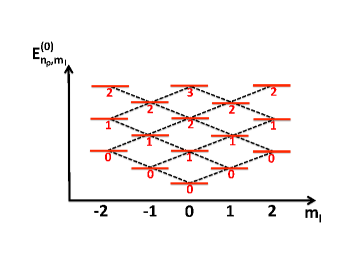
Figure 1: (Color online) Illustration of the selection rules [Eqs. (15) and (18)] for a single particle with spin-orbit coupling of Rashba type. The horizontal solid lines show the unperturbed single particle energies $E_{n_{\rho},m_{l}}^{(0)}$ as a function of the quantum number $m_{l}$. The value of $n_{\rho}$ is given below each energy level. The dotted lines indicate the non-vanishing matrix elements, i.e., the allowed transitions between unperturbed states (see text for details).

Solid horizontal lines show the unperturbed energies $E^{(0)}_{n_{\rho},m_{l}}$ as a function of $m_{l}$. The number below each energy level indicates the principal quantum number $n_{\rho}$. Dotted lines indicate non-vanishing matrix elements. It is important to note that the matrix elements are only non-zero under certain conditions. For example, let us start in the $(n_{\rho}^{\prime},m_{l}^{\prime})=(0,0)$ state. If $m_{s}^{\prime}$ is equal to $1/2$, one can reach the $(n_{\rho},m_{l})=(0,1)$ state (i.e., one can take a step to the right) but one cannot reach the $(n_{\rho},m_{l})=(0,-1)$ state (i.e., one cannot take a step to the left). If $m_{s}^{\prime}$ is equal to $-1/2$, in contrast, one can reach the $(n_{\rho},m_{l})=(0,-1)$ state (i.e., one can take a step to the left) but one cannot reach the $(n_{\rho},m_{l})=(0,1)$ state (i.e., one cannot take a step to the right).

We write the perturbation series as

$$E_{n_{\rho},m_{l},m_{s}}\approx E_{n_{\rho},m_{l}}^{(0)}+\sum_{k=1}^{k_{\text{max}}}\Delta E^{(k)}_{n_{\rho},m_{l},m_{s}},$$ (19)

where the energy shifts $\Delta E^{(k)}_{n_{\rho},m_{l},m_{s}}$ are determined by applying $k$th-order perturbation theory. Energies $E_{n_{\rho},m_{l},m_{s}}$ with the same $E^{(0)}_{n_{\rho},m_{l}}$ and $|m_{j}|$ are degenerate.

The selection rules discussed above imply that the first-order energy shift vanishes. For $k=2$, we have

$$\Delta E_{n_{\rho},m_{l},m_{s}}^{(2)}=\sum_{n_{\rho}^{\prime},m_{l}^{\prime},m_{s}^{\prime}}\frac{|\langle\psi_{n_{\rho},m_{l},m_{s}}^{(0)}|V_{\text{so}}|\psi^{(0)}_{n_{\rho}^{\prime},m_{l}^{\prime},m_{s}^{\prime}}\rangle|^{2}}{E_{n_{\rho},m_{l}}^{(0)}-E_{n_{\rho}^{\prime},m_{l}^{\prime}}^{(0)}},$$ (20)

where the sum excludes states with eigenenergy $E_{n_{\rho},m_{l}}^{(0)}$. The matrix elements that contribute to the second-order perturbation shift of the ground state are illustrated schematically in Figs. 2(a) and 2(b). The matrix elements give a non-zero contribution only for $(n_{\rho}^{\prime},m_{l}^{\prime},m_{s}^{\prime})=(0,1,-1/2)$ if $m_{s}=1/2$ and for $(n_{\rho}^{\prime},m_{l}^{\prime},m_{s}^{\prime})=(0,-1,1/2)$ if $m_{s}=-1/2$.

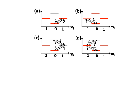
Figure 2: (Color online) Non-zero matrix elements for a single particle with spin-orbit coupling of Rashba type in the ground state at second- and fourth-order perturbation theory. Solid horizontal lines show the unperturbed energies $E_{n_{\rho},m_{l}}^{(0)}$ as a function of $m_{l}$. Arrows in panels (a) and (b) show the “allowed paths” that contribute to the energy shift $\Delta E_{0,0,\pm 1/2}^{(2)}$. Arrows in panels (c) and (d) show the “allowed paths” that contribute to the energy shift $\Delta E_{0,0,\pm 1/2}^{(4)}$.

We find, in agreement with Refs. governale02 ; zinner12 , that the second-order energy shift is given by

$$\Delta E^{(2)}_{n_{\rho},m_{l},m_{s}}=-(1\pm|m_{l}|)E_{\text{so}}$$ (21)

for $|m_{j}|=|m_{l}|\pm 1/2$, where

$$E_{\text{so}}=\frac{\hbar^{2}k_{\text{so}}^{2}}{m}.$$ (22)

We write the $k$th-order perturbation shift ($k$ even) as

$$\Delta E^{(k)}_{n_{\rho},m_{l},m_{s}}=c_{n_{\rho},m_{l},m_{s}}^{(k)}\left(\frac{E_{\text{so}}}{E_{\text{ho}}}\right)^{k/2}E_{\text{ho}}.$$ (23)

We find that $\Delta E_{n_{\rho},m_{l},m_{s}}^{(k)}=0$ for odd $k$ due to the $m_{s}$ selection rule. The $c^{(2)}_{n_{\rho},m_{l},m_{s}}$-coefficients can be read off Eq. (21). Figures  2(c) and 2(d) illustrate the non-zero matrix elements that contribute to the energy shift of the ground state at fourth-order perturbation theory. Evaluating the perturbation expression, we find

$$c^{(4)}_{n_{\rho},m_{l},m_{s}}=(2n_{\rho}+|m_{l}|+1)(1/2\pm|m_{l}|)$$ (24)

for $|m_{j}|=|m_{l}|\pm 1/2$. Table 2 summarizes the $c_{n_{\rho},m_{l},m_{s}}^{(k)}$ coefficients for $k=2,4,\cdots,12$ for the ground state.

Table 2: Coefficients $c_{0,0,\pm 1/2}^{(k)}$ [see Eq. (23)] for a single particle with spin-orbit coupling of Rashba type. The coefficients determine the energy shift for the ground state.

$k$	$c_{0,0,\pm 1/2}^{(k)}$	$k$	$c_{0,0,\pm 1/2}^{(k)}$
2	$-1$	8	$79/72$
4	$1/2$	10	$-274/135$
6	$-2/3$	12	$130577/32400$

We developed an analogous scheme to evaluate the corrections to the unperturbed wave functions. We write

$$\psi_{n_{\rho},m_{l},m_{s}}(\rho,\varphi)\approx N_{n_{\rho},m_{l},m_{s}}\Bigg{\{}\psi^{(0)}_{n_{\rho},m_{l},m_{s}}(\rho,\varphi)+\sum_{k=1}^{k_{\text{max}}}(k_{\text{so}}a_{\text{ho}})^{k}\Bigg{[}\sum_{n_{\rho}^{\prime},m_{l}^{\prime},m_{s}^{\prime}}d^{(n_{\rho},m_{l},m_{s},k)}_{n_{\rho}^{\prime},m_{l}^{\prime},m_{s}^{\prime}}\psi^{(0)}_{n_{\rho}^{\prime},m_{l}^{\prime},m_{s}^{\prime}}(\rho,\varphi)\Bigg{]}\Bigg{\}},$$ (25)

where the quantum numbers $m_{l}^{\prime}$ and $m_{s}^{\prime}$ are constrained by $m_{l}^{\prime}+m_{s}^{\prime}=m_{j}$ and where the sum excludes states with eigenenergy $E^{(0)}_{n_{\rho},m_{l}}$. In Eq. (25), the normalization constant $N_{n_{\rho},m_{l},m_{s}}$ can be readily obtained once the $d_{n_{\rho}^{\prime},m_{l}^{\prime},m_{s}^{\prime}}^{(n_{\rho},m_{l},m_{s},k)}$-coefficients are known,

$$(N_{n_{\rho},m_{l},m_{s}})^{-2}=1+\sum_{n_{\rho}^{\prime},m_{l}^{\prime},m_{s}^{\prime}}\left[\sum_{k=1}^{k_{\text{max}}}(k_{\text{so}}a_{\text{ho}})^{k}d_{n_{\rho}^{\prime},m_{l}^{\prime},m_{s}^{\prime}}^{(n_{\rho},m_{l},m_{s},k)}\right]^{2},$$ (26)

where, as before, the sum excludes terms corresponding to eigenenergies $E^{(0)}_{n_{\rho},m_{l}}$. For $k=1$ and $2$, we derive general expressions for the expansion coefficients,

$$d^{(n_{\rho},m_{l},\pm 1/2,1)}_{n_{\rho}^{\prime},m_{l}^{\prime},m_{s}^{\prime}}=\mp\delta_{m_{s}^{\prime},\mp 1/2}\delta_{m_{l}^{\prime},m_{l}\pm 1}\Bigg{\{}\begin{array}[]{c}\left(\sqrt{n_{\rho}+|m_{l}|+1}\delta_{n_{\rho}^{\prime},n_{\rho}}-\sqrt{n_{\rho}}\delta_{n_{\rho}^{\prime},n_{\rho}-1}\right)\mbox{ for }|m_{j}|=|m_{l}|+1/2\\ \left(\sqrt{n_{\rho}+|m_{l}|}\delta_{n_{\rho}^{\prime},n_{\rho}}-\sqrt{n_{\rho}+1}\delta_{n_{\rho}^{\prime},n_{\rho}+1}\right)\mbox{ for }|m_{j}|=|m_{l}|-1/2\end{array}$$ (29)

and

$$d^{(n_{\rho},m_{l},\pm 1/2,2)}_{n_{\rho}^{\prime},m_{l}^{\prime},m_{s}^{\prime}}=\frac{1}{2}\delta_{m_{s}^{\prime},\pm 1/2}\delta_{m_{l}^{\prime},m_{l}}\bigg{(}\sqrt{(n_{\rho}+|m_{l}|+1)(n_{\rho}+1)}\delta_{n_{\rho}^{\prime},n_{\rho}+1}+\sqrt{n_{\rho}(n_{\rho}+|m_{l}|)}\delta_{n_{\rho}^{\prime},n_{\rho}-1}\bigg{)}.$$ (30)

Table 3: Coefficients $d_{n_{\rho}^{\prime},m_{l}^{\prime},m_{s}^{\prime}}^{(0,0,\pm 1/2,k)}$ [see Eq. (25)] for a single particle with spin-orbit coupling of Rashba type. The coefficients determine the wave function corrections for the ground state with $m_{j}=\pm 1/2$. Columns 2-9 list the coefficients for the non-zero $(n_{\rho}^{\prime},m_{l}^{\prime},m_{s}^{\prime})$ combinations.

$k$	$(0,\pm 1,\mp 1/2)$	$(1,0,\pm 1/2)$	$(1,\pm 1,\mp 1/2)$	$(2,0,\pm 1/2)$	$(2,\pm 1,\mp 1/2)$	$(3,0,\pm 1/2)$	$(3,\pm 1,\mp 1/2)$	$(4,0,\pm 1/2)$
$1$	$\mp 1$
$2$		$1/2$
$3$	$\pm 1/2$		$\mp\sqrt{2}/6$
$4$		$-1/3$		$1/12$
$5$	$\mp 2/3$		$\pm 5\sqrt{2}/36$		$\mp\sqrt{3}/60$
$6$		$35/72$		$-7/90$		$1/120$
$7$	$\pm 31/72$		$\mp 227\sqrt{2}/1080$		$\pm 31\sqrt{3}/1800$		$\mp 1/420$
$8$		$-179/540$		$659/5400$		$-29/3150$		$1/1680$

Table 3 summarizes the $d^{(n_{\rho},m_{l},\pm 1/2,k)}_{n_{\rho}^{\prime},m_{l}^{\prime},m_{s}^{\prime}}$-coefficients for $k=1,2,\cdots,8$ for the ground state, i.e., for $n_{\rho}=0$ and $m_{l}=0$.

To validate our perturbative treatment, we determine the eigenenergies of $H^{(1)}$ ($k_{\text{so}}\geq 0$) numerically following the approach of Ref. pu12 . In the following, we focus on the energies associated with the motion in the $xy$-plane and do not include the energy associated with the motion in the $z$ coordinate. Solid lines in Fig. 3 show the single particle energies as a function of $(k_{\text{so}}a_{\text{ho}})^{2}$.

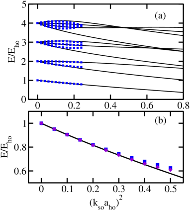
Figure 3: (Color online) Eigenenergies for a single particle with spin-orbit coupling of Rashba type described by the Hamiltonian $H^{(1)}$ (the energy associated with the motion in the $z$ direction has been taken out). (a) Lines show the numerically determined (exact) eigenenergies as a function of $(k_{\text{so}}a_{\text{ho}})^{2}$. Squares show the energies determined perturbatively with $k_{\text{max}}=4$. (b) The ground state energy is shown on an enlarged scale. Squares and diamonds show the energy determined perturbatively with $k_{\text{max}}=4$ and $k_{\text{max}}=12$, respectively.

For comparison, squares show our perturbative energies $E_{n_{\rho},m_{l},m_{s}}$ with $k_{\text{max}}=4$. For the excited states shown, the agreement is excellent for ($k_{\text{so}}a_{\text{ho}})^{2}\lesssim 0.1$. For the ground state [see also the blow-up in Fig. 3(b)], the agreement is excellent for $(k_{\text{so}}a_{\text{ho}})^{2}\lesssim 0.3$. Diamonds in Fig. 3(b) show the perturbative energy for the ground state with $k_{\text{max}}=12$. It can be seen that the inclusion of more terms in the perturbation series improves the agreement with the exact energies in a narrow $k_{\text{so}}a_{\text{ho}}$ window. As expected, as $k_{\text{so}}a_{\text{ho}}$ approaches 1, the perturbative energy expression fails.

III.2 Perturbative treatment of $H^{(12)}_{\text{soc,a}}$: one atom with and one atom without spin-orbit coupling

This section accounts for the atom-atom interaction, modeled using $V_{\text{2b}}^{\uparrow}(\vec{r}_{12})=V_{\text{ps}}^{\uparrow}(\vec{r}_{12})$ and $V_{\text{2b}}^{\downarrow}(\vec{r}_{12})=V_{\text{ps}}^{\downarrow}(\vec{r}_{12})$, perturbatively. We first assume $\omega_{x}=\omega_{y}=\omega_{z}$. We write the unperturbed two-particle wave function as a product of the single particle wave function that accounts for $V_{\text{so}}(\vec{r}_{1})$ perturbatively (see Sec. III.1) and the single particle harmonic oscillator wave function. The former describes the motion of the first particle and is given by Eq. (25) with $\rho=\rho_{1}$ and $\varphi=\varphi_{1}$, multiplied by the one-dimensional harmonic oscillator function $g_{k_{z}}(z_{1})$, where $k_{z}=0,1,\cdots$. The latter describes the motion of the second particle and is given by $R_{N_{\rho},M_{l}}(\rho_{2})\Phi_{M_{l}}(\varphi_{2})$ [see Eqs. (III.1) and (12)], multiplied by the one-dimensional harmonic oscillator function $g_{K_{z}}(z_{2})$, where $K_{z}=0,1,\cdots$. Correspondingly, the unperturbed two-particle energy is given by $E_{n_{\rho},m_{l},m_{s}}+(k_{z}+2N_{\rho}+|M_{l}|+K_{z}+2)\hbar\omega$, where $E_{n_{\rho},m_{l},m_{s}}$ is given in Eq. (19).

Since the atom-atom interaction is spherically symmetric, unperturbed states with the same unperturbed energy but different $M_{J}=m_{l}+m_{s}+M_{l}$ do not couple. To start with, we consider the effect of the atom-atom interaction for case 1a ($a_{\uparrow}=a_{\downarrow}=a_{\text{aa}}$) on the ground state. The first-order energy shift $\Delta E^{(\text{soc,a},1)}_{\text{gr},M_{J}}$ is found by “sandwiching” $H_{\text{soc,a}}^{(12)}$ between the unperturbed states. The matrix elements for states with different $m_{s}$ do not couple. In the following, we consider the matrix element that contains $\psi_{0,0,1/2}$ [Eq. (25)]; considering the matrix element that contains $\psi_{0,0,-1/2}$ yields the same energy shift. Equation (25) and Table 3 show that the term proportional to $(k_{\text{so}})^{0}$ has $m_{s}=1/2$ while the term proportional to $(k_{\text{so}})^{1}$ has $m_{s}=-1/2$. Since these spin states are orthogonal, the energy shift $\Delta E_{\text{gr},M_{J}}^{(\text{soc,a},1)}$ contains a term that is proportional to $a_{\text{aa}}(k_{\text{so}})^{0}$ (in fact, this is the “usual” first-order energy shift one obtains in the absence of spin-orbit coupling busc98 ) but does not contain terms that are proportional to $a_{\text{aa}}k_{\text{so}}$. Moreover, it can be shown readily that the selection rules imply that $\Delta E_{\text{gr},M_{J}}^{(\text{soc,a},1)}$ does not contain terms that are proportional to $a_{\text{aa}}(k_{\text{so}})^{k}$ with $k$ odd.

To calculate the coefficient of the term that is proportional to $a_{\text{aa}}(k_{\text{so}})^{2}$, we have to add up three non-vanishing contributions. The first contribution comes from the fact that the normalization constant $N_{0,0,1/2}$ contains a term that is proportional to $(k_{\text{so}})^{2}$. The second contribution comes from the fact that $\psi_{0,0,1/2}$ contains a term that is proportional to $(k_{\text{so}})^{1}$, which—when squared—gives a non-vanishing contribution. The third contribution comes from the fact that $\psi_{0,0,1/2}$ contains a term that is proportional to $(k_{\text{so}})^{2}$, which—when multiplied by the wave function piece that is proportional to $(k_{\text{so}})^{0}$—gives a non-vanishing contribution. Evaluating these three finite contributions, we find that the sum vanishes, i.e., the energy shift $\Delta E_{\text{gr},M_{J}}^{(\text{soc,a},1)}$ contains no terms that are proportional to $a_{\text{aa}}(k_{\text{so}})^{2}$. We refer to the cancellation of this term as “accidental” and note that the coefficient of the $a_{\text{aa}}(k_{\text{so}})^{2}$ term does, in general, not vanish when one considers excited states (see below).

One might ask whether the fact that the perturbative treatment does not yield a term proportional to $a_{\text{aa}}(k_{\text{so}})^{2}$ for the ground state is a consequence of the azimuthal symmetry. To investigate this question, we consider two situations in which the azimuthal symmetry is broken. We consider the cases where (i) $\omega_{x}\neq\omega_{y}$, and (ii) $\omega_{x}\neq\omega_{y}$ and the Rashba spin-orbit coupling term is anisotropic, i.e., the term proportional to $\partial/\partial x_{1}$ is multiplied by a different constant than the term proportional to $\partial/\partial y_{1}$. In both cases, we find that the energy shift of the ground state does not contain terms that are proportional to $a_{\text{aa}}(k_{\text{so}})^{2}$. This shows that the absence of the coupling between the short-range interaction and the spin-orbit coupling term for the ground state at order $a_{\text{aa}}(k_{\text{so}})^{2}$ is not a consequence of the azimuthal symmetry. Interestingly, we find that the term is also absent in the one-dimensional Hamiltonian with spin-orbit coupling.

Returning to the spherically symmetric harmonic confining potential and isotropic Rashba coupling, we extend the analysis of the ground state to higher orders in $k_{\text{so}}$. We find

$$\Delta E^{(\text{soc,a},1)}_{\text{gr},M_{J}=1/2}=\bigg{[}1+\frac{1}{4}(k_{\text{so}}a_{\text{ho}})^{4}-\frac{23}{36}(k_{\text{so}}a_{\text{ho}})^{6}+$$

$$\frac{1513}{1080}(k_{\text{so}}a_{\text{ho}})^{8}+\cdots\bigg{]}E_{\text{scatt}},$$ (31)

where

$$E_{\text{scatt}}=\sqrt{\frac{2}{\pi}}\frac{a_{\text{aa}}}{a_{\text{ho}}}E_{\text{ho}}.$$ (32)

The first term in the square brackets on the right hand side of Eq. (III.2) is the usual $s$-wave shift busc98 and $E_{\text{scatt}}$ can be interpreted as the “two-particle” mean-field shift. The second term gives the leading-order coupling between the long-range spin-orbit coupling term and the short-range $s$-wave interaction. Generalizing the above analysis to excited states with arbitrary $n_{\rho}$, $m_{l}$ and $m_{s}$ but $N_{\rho}=M_{l}=K_{z}=k_{z}=0$, we find that the first-order energy shift is given by

$$\Delta E^{(\text{soc,a},1)}_{n_{\rho},m_{l},m_{s}}=\bigg{[}\frac{(2n_{\rho}+|m_{l}|)!}{n_{\rho}!(n_{\rho}+|m_{l}|)!2^{2n_{\rho}+|m_{l}|}}+$$

$$\bigg{(}\frac{(2n_{\rho}+|m_{l}|+1)!}{n_{\rho}!(n_{\rho}+|m_{l}|)!2^{2n_{\rho}+|m_{l}|}}-2n_{\rho}-|m_{l}|-1\bigg{)}\times$$

$$(k_{\text{so}}a_{\text{ho}})^{2}+\cdots\bigg{]}E_{\text{scatt}}.$$ (33)

If we allow for different scattering lengths, i.e., if we set $a_{\uparrow}=a_{\text{aa}}$ and $a_{\downarrow}=\eta a_{\text{aa}}$ and assume $\eta\neq 1$ (case 1b), then we find that the first-order energy shift of the unperturbed ground state with $m_{s}=1/2$ ($M_{J}=1/2$) contains terms proportional to $a_{\sigma}(k_{\text{so}})^{2}$,

$$\Delta E_{\text{gr},M_{J}=1/2}^{(\text{soc,a},1)}=\bigg{[}1-\frac{1}{2}(1-\eta)(k_{\text{so}}a_{\text{ho}})^{2}+$$

$$\frac{1}{12}(13-10\eta)(k_{\text{so}}a_{\text{ho}})^{4}-$$

$$\frac{1}{180}(441-326\eta)(k_{\text{so}}a_{\text{ho}})^{6}+$$

$$\frac{1}{37800}(185677-132722\eta)(k_{\text{so}}a_{\text{ho}})^{8}+\cdots\bigg{]}E_{\text{scatt}}.$$ (34)

To get the energy shift $\Delta E_{\text{gr},M_{J}=-1/2}^{(\text{soc,a},1)}$ of the unperturbed ground state with $m_{s}=-1/2$ ($M_{J}=-1/2$), we replace $\eta$ by $1/\eta$ and $E_{\text{scatt}}$ by $\eta E_{\text{scatt}}$ in Eq. (III.2). Equations (III.2) and (III.2) show that the interplay between the short-range interaction and the spin-orbit coupling term is highly tunable. Specifically, the order at which the coupling arises as well as whether the interplay leads to a decrease or increase of the energy can be varied by tuning the $s$-wave scattering lengths.

To validate the perturbative energy shifts given in Eqs. (III.2) and (III.2), we determine the eigenenergies of the Hamiltonian $H_{\text{soc,a}}$ numerically. We denote the numerically obtained two-body ground state energy by $E_{\text{gr}}^{\text{num}}$. As discussed in the Appendix, the basis set expansion approach employs a Gaussian model potential with finite range $r_{0}$ ($r_{0}=0.02a_{\text{ho}}$); this implies that a meaningful comparison of the numerical and perturbative energies has to account for finite-range effects. To isolate the interplay between the spin-orbit coupling term and the $s$-wave interaction, we define the energy difference $\Delta E_{\text{gr}}^{\text{num}}$,

$$\Delta E_{\text{gr}}^{\text{num}}=E_{\text{gr}}^{\text{num}}-E_{\text{gr}}^{s-\text{wave}}-E_{\text{gr}}^{\text{so}}+3\hbar\omega.$$ (35)

Here, $E_{\text{gr}}^{s-\text{wave}}$ denotes the two-body ground state energy calculated for $k_{\text{so}}=0$ using the same finite-range interaction model as used to calculate $E_{\text{gr}}^{\text{num}}$. The energy $E_{\text{gr}}^{s-\text{wave}}$ is obtained with high accuracy numerically by solving the one-dimensional scaled radial Schrödinger equation. In Eq. (35), $E_{\text{gr}}^{\text{so}}$ denotes the two-body ground state energy calculated in the absence of the two-body interaction using the same spin-orbit coupling term as used to calculate $E_{\text{gr}}^{\text{num}}$. As discussed in the context of Fig. 3, the energy $E_{\text{gr}}^{\text{so}}$ can be obtained with high accuracy numerically. For $k_{\text{so}}=0$, our definition implies that $\Delta E_{\text{gr}}^{\text{num}}$ is equal to zero. For finite $k_{\text{so}}$, $\Delta E_{\text{gr}}^{\text{num}}$ reflects the interplay between the spin-orbit coupling term and the $s$-wave interaction.

Figure 4 considers the case where $a_{\uparrow}=a_{\downarrow}=a_{\text{aa}}=-a_{\text{ho}}/10$ (case 1a). The circles show the quantity $\Delta E_{\text{gr}}^{\text{num}}/|E_{\text{scatt}}|$ as a function of $(k_{\text{so}}a_{\text{ho}})^{2}$. $E_{\text{gr}}^{\text{num}}$ equals $2.922770(6)\hbar\omega$ for $(k_{\text{so}}a_{\text{ho}})^{2}=0$ and $2.773036(5)\hbar\omega$ for $(k_{\text{so}}a_{\text{ho}})^{2}=0.16$ while $E_{\text{gr}}^{\text{so}}$ equals $2.8506264\hbar\omega$ for $(k_{\text{so}}a_{\text{ho}})^{2}=0.16$. We estimate that the basis set extrapolation error for the quantity $\Delta E_{\text{gr}}^{\text{num}}/|E_{\text{scatt}}|$ is less than $7\times 10^{-5}$. For comparison, dotted, dashed and solid lines show the perturbative expression $(\Delta E_{\text{gr},M_{J}=1/2}^{(\text{soc,a},1)}-E_{\text{scatt}})/|E_{\text{scatt}}|$, see Eq. (III.2), as a function of $(k_{\text{so}}a_{\text{ho}})^{2}$ up to order $(k_{\text{so}}a_{\text{ho}})^{4}$, $(k_{\text{so}}a_{\text{ho}})^{6}$ and $(k_{\text{so}}a_{\text{ho}})^{8}$, respectively. The inclusion of more terms in the perturbation series systematically improves the agreement with the numerically determined energy shift. Equation (III.2) accounts for the energy shift proportional to $a_{\text{aa}}$ but not for energy shifts proportional to $(a_{\text{aa}})^{j}$ with $j\geq 2$. We find that the leading term in the $(a_{\text{aa}})^{2}$ series [see Eq. (52) of Sec. IV.2] is, for the $k_{\text{so}}a_{\text{ho}}$ considered in Fig. 4, roughly an order of magnitude smaller than the smallest contribution included in Eq. (III.2). For example, the energy shift proportional to $(a_{\text{aa}})^{2}(k_{\text{so}})^{4}$ is $-8\times 10^{-5}|E_{\text{scatt}}|$ for $(k_{\text{so}}a_{\text{ho}})^{2}=0.16$.

Figure 5 considers the case where $a_{\uparrow}=a_{\text{aa}}=-a_{\text{ho}}/6$ and $a_{\downarrow}=\eta a_{\text{aa}}=-a_{\text{ho}}/10$ (case 1b). Circles show the quantity $\Delta E_{\text{gr}}^{\text{num}}$. As shown in Eq. (III.2), the leading-order energy shift that accounts for the interplay between the spin-orbit coupling term and the $s$-wave interaction is proportional to $a_{\text{aa}}(k_{\text{so}})^{2}$ (see the dash-dotted line in Fig. 5). When terms up to order $(k_{\text{so}}a_{\text{ho}})^{8}$ are included (see the solid line in Fig. 5), the first-order perturbation theory shift proportional to $a_{\text{aa}}$ agrees reasonably well with the numerical data. Since $|a_{\text{aa}}|/a_{\text{ho}}$ is appreciable ($a_{\text{aa}}/a_{\text{ho}}=-1/6$), higher-order corrections in $a_{\text{aa}}$ are non-negligible. The dash-dot-dotted line in Fig. 5, which additionally includes higher-order corrections in $a_{\text{aa}}$ [see Eq. (51) in Sec. IV.2], notably improves the agreement with the numerically determined energy shift.

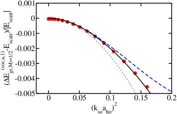
Figure 4: (Color online) Interplay between the $s$-wave interaction and the spin-orbit coupling term for the ground state for one atom with and one atom without spin-orbit coupling (case 1a with $a_{\uparrow}=a_{\downarrow}=a_{\text{aa}}=-a_{\text{ho}}/10$). The lines show the perturbative expression $(\Delta E_{\text{gr},M_{J}=1/2}^{(\text{soc,a},1)}-E_{\text{scatt}})/|E_{\text{scatt}}|$, see Eq. (III.2), as a function of $(k_{\text{so}}a_{\text{ho}})^{2}$. The dotted, dashed and solid lines show the terms up to order $(k_{\text{so}}a_{\text{ho}})^{4}$, $(k_{\text{so}}a_{\text{ho}})^{6}$ and $(k_{\text{so}}a_{\text{ho}})^{8}$, respectively. For comparison, the circles show the quantity $\Delta E_{\text{gr}}^{\text{num}}/|E_{\text{scatt}}|$, see Eq. (35).

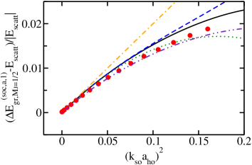
Figure 5: (Color online) Interplay between the $s$-wave interaction and the spin-orbit coupling term for the ground state for one atom with and one atom without spin-orbit coupling (case 1b with $a_{\uparrow}=a_{\text{aa}}=-a_{\text{ho}}/6$ and $a_{\downarrow}=\eta a_{\text{aa}}=-a_{\text{ho}}/10$). The lines show the perturbative expression $(\Delta E_{\text{gr},M_{J}=1/2}^{(\text{soc,a},1)}-E_{\text{scatt}})/|E_{\text{scatt}}|$, see Eq. (III.2), as a function of $(k_{\text{so}}a_{\text{ho}})^{2}$. The dash-dotted, dotted, dashed and solid lines show the expression including terms up to order $(k_{\text{so}}a_{\text{ho}})^{2}$, $(k_{\text{so}}a_{\text{ho}})^{4}$, $(k_{\text{so}}a_{\text{ho}})^{6}$ and $(k_{\text{so}}a_{\text{ho}})^{8}$, respectively. The dash-dot-dotted line additionally includes higher-order corrections in $a_{\text{aa}}$ (see Sec. IV.2 for the derivation of these higher-order corrections). For comparison, the circles show the quantity $\Delta E_{\text{gr}}^{\text{num}}/|E_{\text{scatt}}|$, see Eq. (35).

Figures 4 and 5 report the energy shift that reflects the interplay between the spin-orbit coupling term and the $s$-wave interaction in terms of the quantity $|E_{\text{scatt}}|$, i.e., in terms of the absolute value of the leading-order mean-field shift. In Figs. 4 and 5, the quantity $|(\Delta E_{\text{gr},M_{J}=1/2}^{(\text{soc,a},1)}-E_{\text{scatt}})/E_{\text{scatt}}|$ is smaller than $5\times 10^{-3}$ and $4\times 10^{-2}$, respectively, implying that the energy shift due to the interplay between the spin-orbit coupling term and the $s$-wave interaction is respectively less than a percent and a few percent of the mean-field shift. While these effects are small, they can potentially be measured in “quantum phase revival experiments” analogous to those for few-atom systems in an optical lattice bloch10 . In that work, it was possible to deduce the effective three-body interaction energy, which was measured to be roughly 10 times smaller in absolute value than the effective two-body interaction energy. Moreover, the effective four-body energy was measured to be roughly a factor of 100 smaller than the effective two-body interaction. To probe the interplay between the spin-orbit coupling term and the $s$-wave interaction experimentally, one would compare the oscillation periods in revival experiments with and without spin-orbit coupling.

The treatment discussed in this section can, in principle, be extended to second- and higher-order perturbation theory. However, the use of the interaction model $V_{\text{ps}}^{\sigma}(\vec{r}_{12})$ gives rise, at second- and higher-order perturbation theory, to divergencies that need to be removed through application of a renormalization scheme. Although this can be done via standard techniques (see, e.g., Refs. NJP1 ; NJP2 ), we find it easier to determine the energy shifts that are proportional to $(a_{\text{aa}})^{2}(k_{\text{so}})^{2}$ and $(a_{\text{aa}})^{2}(k_{\text{so}})^{4}$ by an approach that builds on the exact two-particle $s$-wave solution (see Sec. IV).

The key points of this section are:

• For the ground state manifold, the perturbative energy shifts contain even but not odd powers of $k_{\text{so}}a_{\text{ho}}$.

• For $a_{\uparrow}=a_{\downarrow}=a_{\text{aa}}$ ($\eta=1$), the energy shift proportional to $a_{\text{aa}}(k_{\text{so}})^{2}$ vanishes for the ground state. This finding does not only hold for isotropic Rashba coupling and isotropic traps, but also for anisotropic Rashba coupling and/or anisotropic harmonic traps. In general, the energy shift proportional to $a_{\text{aa}}(k_{\text{so}})^{2}$ does not vanish for excited states [see Eqs. (III.2) and (III.2)].

• For $a_{\uparrow}=a_{\text{aa}}\neq a_{\downarrow}$ ($\eta\neq 1$), the leading-order energy shifts of the states in the lowest energy manifold due to the interplay between the spin-orbit coupling term and the $s$-wave interaction are proportional to $a_{\text{aa}}(k_{\text{so}})^{2}$.

III.3 Perturbative treatment of $H^{(12)}_{\text{soc,soc}}$: Two particles with spin-orbit coupling

This section considers the situation where both particles feel the Rashba spin-orbit coupling. Throughout, we assume $\omega_{x}=\omega_{y}=\omega_{z}$. We write the unperturbed two-particle wave function as a product of two single-particle wave functions, which account for the spin-orbit coupling terms $V_{\text{so}}(\vec{r}_{1})$ and $V_{\text{so}}(\vec{r}_{2})$ perturbatively. For concreteness, we focus on the ground state manifold that consists of the unperturbed wavefunctions $\Psi^{(0)}_{m_{s1},m_{s2}}$, where $\Psi^{(0)}_{m_{s1},m_{s2}}=\psi_{0,0,m_{s1}}(\rho_{1},\varphi_{1})g_{0}(z_{1})\psi_{0,0,m_{s2}}(\rho_{2},\varphi_{2})g_{0}(z_{2})$ and $(m_{s1},m_{s2})=(1/2,1/2),(-1/2,-1/2),(1/2,-1/2)$ and $(-1/2,1/2)$. As before, $\psi$ is given by Eq. (25) and $g_{0}$ denotes the one-dimensional harmonic oscillator function with energy $\hbar\omega/2$. The four degenerate unperturbed wave functions are eigenstates of the total $J_{z}$ operator with eigenvalue $\hbar M_{J}$ ($M_{J}=m_{l1}+m_{s1}+m_{l2}+m_{s2}$ or, equivalently, $M_{J}=m_{j1}+m_{j2}$), where $M_{J}=1,-1,0$ and $0$, respectively. Since $M_{J}$ is a good quantum number, the perturbation $H^{(12)}_{\text{soc,soc}}$ only couples states with the same $M_{J}$. In what follows, we use $V_{\text{2b}}^{\sigma\sigma^{\prime}}(\vec{r}_{12})=V_{\text{ps}}^{\sigma\sigma^{\prime}}(\vec{r}_{12})$ and treat $H_{\text{soc,soc}}^{(12)}$ in first-order perturbation theory.

We start by considering case 2d ($\zeta,\eta\neq 1$ and $\zeta\neq\eta$). For the state with $M_{J}=1$, the first-order energy shift in the scattering length is given by

$$\Delta E^{(\text{soc,soc},1)}_{\text{gr},M_{J}=1(S)}=\bigg{[}1-\left(1-\eta\right)(k_{\text{so}}a_{\text{ho}})^{2}+$$

$$\frac{1}{6}\left(16+3\zeta-16\eta\right)(k_{\text{so}}a_{\text{ho}})^{4}-$$

$$\frac{1}{90}\left(606+165\zeta-656\eta\right)(k_{\text{so}}a_{\text{ho}})^{6}+$$

$$\frac{1}{37800}\left(589229+215250\zeta-693844\eta\right)(k_{\text{so}}a_{\text{ho}})^{8}+$$

$$\cdots\bigg{]}E_{\text{scatt}},$$ (36)

where $E_{\text{scatt}}$ is defined in Eq. (32). The subscript “$(S)$” indicates that the corresponding eigenstate is symmetric under the exchange of particles 1 and 2. Similarly, for the state with $M_{J}=-1$, the first-order energy shift $\Delta E^{(\text{soc,soc},1)}_{\text{gr},M_{J}=-1(S)}$ is given by Eq. (III.3) with $\zeta$ replaced by $1/\zeta$, $\eta$ replaced by $\eta/\zeta$ and $E_{\text{scatt}}$ replaced by $\zeta E_{\text{scatt}}$.

We find that the two states with $M_{J}=0$ couple. This means that we have to employ first-order degenerate perturbation theory. The diagonal elements $\langle\Psi^{(0)}_{1/2,-1/2}|H^{(12)}_{\text{soc,soc}}|\Psi^{(0)}_{1/2,-1/2}\rangle$ and $\langle\Psi^{(0)}_{-1/2,1/2}|H^{(12)}_{\text{soc,soc}}|\Psi^{(0)}_{-1/2,1/2}\rangle$ of the perturbation matrix are given by Eq. (III.3) with $\zeta$ replaced by $1$, $\eta$ replaced by $(1/\eta+\zeta/\eta)/2$ and $E_{\text{scatt}}$ replaced by $\eta E_{\text{scatt}}$. For the off-diagonal elements, we find

$$\langle\Psi^{(0)}_{1/2,-1/2}|H^{(12)}_{\text{soc,soc}}|\Psi_{-1/2,1/2}^{(0)}\rangle=$$

$$\langle\Psi^{(0)}_{-1/2,1/2}|H^{(12)}_{\text{soc,soc}}|\Psi_{1/2,-1/2}^{(0)}\rangle=$$

$$\bigg{[}\frac{1}{2}(k_{\text{so}}a_{\text{ho}})^{2}-\frac{4}{3}(k_{\text{so}}a_{\text{ho}})^{4}+\frac{164}{45}(k_{\text{so}}a_{\text{ho}})^{6}-$$

$$\frac{173461}{18900}(k_{\text{so}}a_{\text{ho}})^{8}+\cdots\bigg{]}\left(1+\zeta-2\eta\right)E_{\text{scatt}}.$$ (37)

Diagonalizing the $2\times 2$ perturbation matrix, we find

$$\Delta E^{(\text{soc,soc},1)}_{\text{gr},M_{J}=0(S)}=\bigg{[}\eta+\left(1+\zeta-2\eta\right)(k_{\text{so}}a_{\text{ho}})^{2}-$$

$$\frac{1}{6}\left(16+16\zeta-35\eta\right)(k_{\text{so}}a_{\text{ho}})^{4}+$$

$$\frac{1}{90}\left(656+656\zeta-1427\eta\right)(k_{\text{so}}a_{\text{ho}})^{6}-$$

$$\frac{1}{37800}\left(693844+693844\zeta-1498323\eta\right)(k_{\text{so}}a_{\text{ho}})^{8}$$

$$+\cdots\bigg{]}E_{\text{scatt}}$$ (38)

and

$$\Delta E^{(\text{soc,soc},1)}_{\text{gr},M_{J}=0(A)}=\bigg{[}1+\frac{1}{2}(k_{\text{so}}a_{\text{ho}})^{4}-\frac{23}{18}(k_{\text{so}}a_{\text{ho}})^{6}+$$

$$\frac{3161}{1080}(k_{\text{so}}a_{\text{ho}})^{8}+\cdots\bigg{]}\eta E_{\text{scatt}}.$$ (39)

The corresponding eigenstates are $(\Psi^{(0)}_{1/2,-1/2}+\Psi^{(0)}_{-1/2,1/2})/\sqrt{2}$ and $(\Psi^{(0)}_{1/2,-1/2}-\Psi^{(0)}_{-1/2,1/2})/\sqrt{2}$, respectively. The former state is symmetric under the exchange of particles 1 and 2, while the latter is anti-symmetric under the exchange of particles 1 and 2. The symmetry of the states is indicated by the subscripts “$(S)$” and “$(A)$” in Eqs. (III.3) and (III.3), respectively.

Our calculations imply that the ground state manifold for two identical bosons contains three states, whose energy shifts are given by Eq. (III.3), Eq. (III.3) with the substitutions discussed below the equation and Eq. (III.3). For two identical fermions, the ground state manifold contains a single state, whose energy shift is given by Eq. (III.3). As expected, the energy shift corresponding to the anti-symmetric state is independent of $a_{\uparrow\uparrow}$ and $a_{\downarrow\downarrow}$. Although our interaction model allows for $s$-wave scattering in all four channels (up-up, down-down, up-down, down-up), the anti-symmetry of the wave function “turns off” the interactions in the up-up and down-down channels, yielding an energy shift that is fully determined by $a_{\uparrow\downarrow}=a_{\downarrow\uparrow}=\eta a_{\text{aa}}$. The energy shifts corresponding to the three symmetric states contain a term proportional to $(k_{\text{so}}a_{\text{ho}})^{2}$ while the energy shift corresponding to the anti-symmetric state does not contain a term proportional to $(k_{\text{so}}a_{\text{ho}})^{2}$.

While our derivation above assumed $\zeta,\eta\neq 1$ and $\zeta\neq\eta$ (case 2d), the energy shifts for cases 2a-2c can be obtained by taking the appropriate limits in Eqs. (III.3)-(III.3). In the limit that $\zeta=1$ and $\eta\neq 1$ (case 2b), the energy shifts of the two $|M_{J}|=1$ states with bosonic exchange symmetry are equal to each other and contain terms proportional to $a_{\text{aa}}(k_{\text{so}})^{2}$. The $M_{J}=0$ state with bosonic exchange symmetry also contains a shift proportional to $a_{\text{aa}}(k_{\text{so}})^{2}$. In the limit that $\zeta\neq 1$ and $\eta=1$ (case 2c), the energy shift of the $M_{J}=1$ state contains no term proportional to $a_{\text{aa}}(k_{\text{so}})^{2}$ while the energy shift of the $M_{J}=-1$ and $M_{J}=0$ states with bosonic exchange symmetry contain terms proportional to $a_{\text{aa}}(k_{\text{so}})^{2}$. In the limit that $\zeta=\eta=1$ (case 2a), the degeneracy of the unperturbed states is preserved, i.e., the four energy shifts of the ground state manifold are all equal to each other and given by Eq. (III.3). In this case, the energy shift of the ground state contains no terms that are proportional to $a_{\text{aa}}(k_{\text{so}})^{2}$. Interestingly, the energy shift given in Eq. (III.3) is nearly identical to the shift given in Eq. (III.2) for the two-atom system where only one of the particles feels the spin-orbit coupling. Specifically, terms proportional to $(k_{\text{so}}a_{\text{ho}})^{4}$ and $(k_{\text{so}}a_{\text{ho}})^{6}$ differ by a factor of 2, reflecting the fact that the interplay between the spin-orbit coupling term and the $s$-wave interaction scales with the number of particles that feel the spin-orbit coupling term. At order $(k_{\text{so}}a_{\text{ho}})^{8}$, the two expressions differ by a factor different from 2, indicating that the interplay between the spin-orbit coupling term and the $s$-wave interaction is not simply additive at higher orders.

To illustrate the behavior of the energy level structure of the ground state manifold for two identical particles, we focus on systems with $\zeta=1$. Lines in Fig. 6 show the quantity $\Delta E_{\text{gr},M_{J}}^{(\text{soc,soc},1)}/E_{\text{scatt}}$ as a function of $(k_{\text{so}}a_{\text{ho}})^{2}$ for (a) $\eta=0.8$, (b) $\eta=1$ and (c) $\eta=1.2$. For $\eta=1$ [case 2a, Fig. 6(b)], the four energy shifts for the states with $M_{J}=0$ and $\pm 1$ are the same (see discussion above). For $\eta=0.8$ [case 2b, Fig. 6(a)], the $M_{J}=0$ state with fermionic exchange symmetry has lower energy if $a_{\text{aa}}>0$ while the two-fold degenerate $|M_{J}|=1$ states with bosonic exchange symmetry have lower energy if $a_{\text{aa}}<0$. For $\eta=1.2$ [Fig. 6(c)], the two-fold degenerate $|M_{J}|=1$ states with bosonic exchange symmetry have lower energy if $a_{\text{aa}}>0$ while the $M_{J}=0$ state with fermionic exchange symmetry has lower energy if $a_{\text{aa}}<0$.

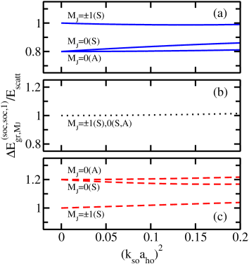
Figure 6: (Color online) First-order energy shift $\Delta E^{(\text{soc,soc},1)}_{\text{gr},M_{J}}$ for the ground state manifold for two identical particles with spin-orbit coupling (case 2a with $\zeta=1$ and $\eta=1$, and case 2b with $\zeta=1$ and $\eta\neq 1$). Solid, dotted and dashed lines show the quantity $\Delta E^{(\text{soc,soc},1)}_{\text{gr},M_{J}}/E_{\text{scatt}}$ [see Eqs. (III.3), (III.3) and (III.3)] as a function of $(k_{\text{so}}a_{\text{ho}})^{2}$ for (a) $\eta=0.8$, (b) $\eta=1$ and (c) $\eta=1.2$, respectively. The energy levels are labeled by the $M_{J}$ quantum number and the exchange symmetry ($S/A$) of the corresponding states.

Figure 7 compares the perturbative predictions (lines) with our numerical basis set expansion results (circles). Figure 7(a) shows an example for $a_{\text{aa}}=-a_{\text{ho}}/10$ and $\zeta=\eta=1$ (case 2a). In this case, the ground state is four-fold degenerate and the term proportional to $a_{\text{aa}}(k_{\text{so}})^{2}$ is absent. Figure 7(b) shows the case where $a_{\text{aa}}=-a_{\text{ho}}/6$, $\zeta=1$ and $\eta a_{\text{aa}}=-a_{\text{ho}}/10$ (case 2b). According to the analysis above, the lowest energy state is two-fold degenerate ($|M_{J}|=1$) and possesses bosonic exchange symmetry. The leading-order energy shift is proportional to $a_{\text{aa}}(k_{\text{so}})^{2}$. Figure 7(c) shows the case where $a_{\text{aa}}=-a_{\text{ho}}/10$, $\zeta=1$ and $\eta a_{\text{aa}}=-a_{\text{ho}}/6$ (case 2b). According to the analysis above, the lowest energy state is one-fold degenerate ($M_{J}=0$) and possesses fermionic exchange symmetry. The energy shift is given by Eq. (III.3), where the term proportional to $a_{\text{aa}}(k_{\text{so}})^{2}$ is again absent footnote . Figure 7 demonstrates excellent agreement between the perturbative predictions and our numerical results for all cases.

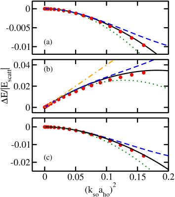
Figure 7: (Color online) Interplay between the $s$-wave interaction and the spin-orbit coupling term for the ground state manifold for two atoms with spin-orbit coupling. (a) The dotted, dashed and solid lines show the expression $(\Delta E_{\text{gr},M_{J}=1(S)}^{(\text{soc,soc},1)}-E_{\text{scatt}})/|E_{\text{scatt}}|$, Eq. (III.3), for the lowest energy state including terms up to order $(k_{\text{so}}a_{\text{ho}})^{4}$, $(k_{\text{so}}a_{\text{ho}})^{6}$ and $(k_{\text{so}}a_{\text{ho}})^{8}$, respectively, as a function of $(k_{\text{so}}a_{\text{ho}})^{2}$ for case 2a with $a_{\text{aa}}=-a_{\text{ho}}/10$, $\zeta=1$ and $\eta=1$. (b) The dash-dotted, dotted, dashed and solid lines show the expression $(\Delta E_{\text{gr},M_{J}=1(S)}^{(\text{soc,soc},1)}-E_{\text{scatt}})/|E_{\text{scatt}}|$, Eq. (III.3), for the lowest energy state including terms up to order $(k_{\text{so}}a_{\text{ho}})^{2}$, $(k_{\text{so}}a_{\text{ho}})^{4}$, $(k_{\text{so}}a_{\text{ho}})^{6}$ and $(k_{\text{so}}a_{\text{ho}})^{8}$, respectively, as a function of $(k_{\text{so}}a_{\text{ho}})^{2}$ for case 2b with $a_{\text{aa}}=-a_{\text{ho}}/6$, $\zeta=1$ and $\eta a_{\text{aa}}=-a_{\text{ho}}/10$. (c) The dotted, dashed and solid lines show the expression $(\Delta E_{\text{gr},M_{J}=0(A)}^{(\text{soc,soc},1)}-\eta E_{\text{scatt}})/|E_{\text{scatt}}|$, Eq. (III.3), for the ground state including terms up to order $(k_{\text{so}}a_{\text{ho}})^{4}$, $(k_{\text{so}}a_{\text{ho}})^{6}$ and $(k_{\text{so}}a_{\text{ho}})^{8}$, respectively, as a function of $(k_{\text{so}}a_{\text{ho}})^{2}$ for case 2b with $a_{\text{aa}}=-a_{\text{ho}}/10$, $\zeta=1$ and $\eta a_{\text{aa}}=-a_{\text{ho}}/6$. For comparison, the circles show the quantity $\Delta E_{\text{gr}}^{\text{num}}/|E_{\text{scatt}}|$, see Eq. (35).

The key points of this section are:

• For the ground state manifold, the perturbative energy shifts contain even but not odd powers of $k_{\text{so}}a_{\text{ho}}$.

• For two identical bosons, the energy shift proportional to $a_{\text{aa}}(k_{\text{so}})^{2}$ is non-zero for the ground state unless the scattering lengths in the four spin channels are such that $a_{\uparrow\uparrow}=a_{\uparrow\downarrow}=a_{\downarrow\uparrow}$ ($1-\eta=0$) or $a_{\uparrow\uparrow}+a_{\downarrow\downarrow}-2a_{\uparrow\downarrow}=0$ ($1+\zeta-2\eta=0$).

• For two identical fermions, the energy shift of the ground state does not contain a term proportional to $a_{\text{aa}}(k_{\text{so}})^{2}$.

IV Arbitrary atom-atom scattering length and weak spin-orbit coupling

This section takes advantage of the fact that the solution for two particles without spin-orbit coupling under external spherically symmetric confinement interacting through the regularized pseudopotential $V_{\text{ps,reg}}(\vec{r}_{12})$ is known in compact analytical form for arbitrary $s$-wave scattering length busc98 . Motivated by this, we treat the spin-orbit coupling perturbatively. Section IV.1 reviews the solution for two particles without spin-orbit coupling. The two-particle energy spectrum for $k_{\text{so}}=0$ is shown in Fig. 8(b) as a function of the inverse of the $s$-wave scattering length. Sections IV.2-IV.4 discuss, using the exact two-body $s$-wave solution, the perturbative treatment of $V_{\text{so}}(\vec{r}_{1})$ and $V_{\text{so}}(\vec{r}_{1})+V_{\text{so}}(\vec{r}_{2})$. Section IV.2 treats the system where one particle does and the other does not feel the spin-orbit coupling term assuming small $|k_{\text{so}}|a_{\text{ho}}$ but arbitrary $s$-wave scattering lengths. Equations (50)-(IV.2) contain the resulting perturbative energy expressions, which are applicable when the states in the manifold studied are not degenerate with other states. Figures 9/12 and 10/11 respectively illustrate and validate these perturbative results. The regime where states in the manifold studied are degenerate with other states is studied in Sec. IV.3 via near-degenerate perturbation theory for selected examples (see Fig. 13 for an illustration of the results). Lastly, Sec. IV.4 treats the system where both particles feel the spin-orbit coupling term assuming small $|k_{\text{so}}|a_{\text{ho}}$ but arbitrary $s$-wave scattering lengths. Equations (61)-(63) contain the resulting perturbative energy expressions and Fig. 15 validates these results through comparison with “exact” numerical energies.

IV.1 Two-body wave function for arbitrary atom-atom scattering length

Throughout, we assume $\omega_{x}=\omega_{y}=\omega_{z}$. In this case, the two-body solution for two particles without spin-orbit coupling and arbitrary $a_{\text{aa}}$ is most conveniently written in terms of the relative distance vector $\vec{r}_{12}$ and the center of mass vector $\vec{R}_{12}$, $\vec{R}_{12}=(\vec{r}_{1}+\vec{r}_{2})/2$. Specifically, the total two-body wave function can be written as a product of the relative wave function $\psi_{q_{\text{rel}},l_{\text{rel}},m_{\text{rel}}}^{\text{rel}}$ and the center of mass wave function $\psi^{\text{cm}}_{N_{\text{cm}},M_{\text{cm}},K_{\text{cm}}}$, and the two-particle energy is given by the sum of the relative and center of mass contributions.

The relative wave function is obtained by solving the relative Schrödinger equation using spherical coordinates. For relative orbital angular momentum $l_{\text{rel}}=0$ and corresponding projection quantum number $m_{\text{rel}}=0$, the relative wave function reads busc98

$$\psi_{q_{\text{rel}},0,0}^{\text{rel}}(\vec{r}_{12})=\frac{N_{q_{\text{rel}}}}{\sqrt{4\pi}}U\left(-q_{\text{rel}},\frac{3}{2},\frac{1}{2}\left[\frac{r_{12}}{a_{\text{ho}}}\right]^{2}\right)\times$$

$$e^{-\frac{1}{4}\left(\frac{r_{12}}{a_{\text{ho}}}\right)^{2}},$$ (40)

where $U$ is the confluent hypergeometric function and $N_{q_{\text{rel}}}$ is the normalization constant [see Eq. (B3) of Ref. daily12 for an explicit expression for $N_{q_{\text{rel}}}$; see also Ref. busc98 ]. The allowed non-integer quantum numbers $q_{\text{rel}}$ are obtained by solving the transcendental equation busc98

$$\frac{\sqrt{2}\Gamma(-q_{\text{rel}})}{\Gamma(-q_{\text{rel}}-1/2)}=\frac{a_{\text{ho}}}{a_{\text{aa}}}.$$ (41)

The relative $l_{\text{rel}}=0$ eigenenergies are given by $(2q_{\text{rel}}+3/2)\hbar\omega$. Figure 8(a) illustrates the relationship between $q_{\text{rel}}$ and $a_{\text{aa}}$. In the non-interacting regime, e.g., one finds $q_{\text{rel}}=0,1,2,\cdots$; for $|a_{\text{aa}}|=\infty$, in contrast, one finds $q_{\text{rel}}=-1/2,1/2,3/2,\cdots$. The relative states with $l_{\text{rel}}>0$ are not affected by the $s$-wave interaction and are given by the three-dimensional harmonic oscillator states with quantum numbers $n_{\text{rel}}$, $l_{\text{rel}}$ and $m_{\text{rel}}$.

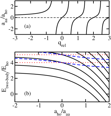
Figure 8: (Color online) Energy spectrum for two particles without spin-orbit coupling and arbitrary $a_{\text{aa}}$. (a) The solid lines show $a_{\text{aa}}/a_{\text{ho}}$ as a function of the non-integer quantum number $q_{\text{rel}}$. $q_{\text{rel}}$ takes on integer values when $a_{\text{aa}}=0$ and half-integer values when $1/a_{\text{aa}}=0$. The dashed line shows the “zero line”. (b) Lines show the two-body energy $E_{\text{two-body}}$ as a function of $a_{\text{ho}}/a_{\text{aa}}$. The solid and dashed lines show the energies of states with $l_{\text{rel}}=0$ while the dotted lines show the energies of states with $l_{\text{rel}}>0$. The lowest solid and lowest dashed lines show energies of states without center of mass excitations.

The center of mass wave functions $\psi^{\text{cm}}_{N_{\text{cm}},M_{\text{cm}},K_{\text{cm}}}$ coincide with the three-dimensional harmonic oscillator states. Since the center of mass wave functions are conveniently written in cylindrical coordinates, we use the quantum numbers $N_{\text{cm}}$, $M_{\text{cm}}$ and $K_{\text{cm}}$ with $N_{\text{cm}}$ and $K_{\text{cm}}=0,1,\cdots$ and $M_{\text{cm}}=0,\pm 1,\cdots$ as labels. Figure 8(b) shows the two-particle energy spectrum as a function of $a_{\text{ho}}/a_{\text{aa}}$. Energy levels corresponding to states with $l_{\text{rel}}=0$ are shown by solid and dashed lines while those corresponding to $l_{\text{rel}}>0$ are shown by dotted lines. The following sections investigate how the spin-orbit coupling term modifies the energy spectrum shown in Fig. 8(b).

IV.2 Perturbative treatment of $V_{\text{so}}(\vec{r}_{1})$: One atom with and one atom without spin-orbit coupling

To treat the spin-orbit term $V_{\text{so}}(\vec{r}_{1})$ perturbatively, we transform it to relative and center of mass coordinates,

$$V_{\text{so}}(\vec{r}_{1})=V_{\text{so}}^{\text{rel},1}(\vec{r}_{12})+V_{\text{so}}^{\text{cm},1}(\vec{R}_{12}),$$ (42)

where

$$V_{\text{so}}^{\text{rel},1}(\vec{r}_{12})=-\imath\frac{\hbar^{2}k_{\text{so}}}{m}\times$$

$$\Bigg{[}\left(\frac{\partial}{\partial y_{12}}+\imath\frac{\partial}{\partial x_{12}}\right)|\uparrow\rangle_{1}\,{}_{1}\langle\downarrow|+$$

$$\left(\frac{\partial}{\partial y_{12}}-\imath\frac{\partial}{\partial x_{12}}\right)|\downarrow\rangle_{1}\,{}_{1}\langle\uparrow|\Bigg{]}$$ (43)

and

$$V_{\text{so}}^{\text{cm},1}(\vec{R}_{12})=-\imath\frac{\hbar^{2}k_{\text{so}}}{2m}\times$$

$$\Bigg{[}\left(\frac{\partial}{\partial Y_{12}}+\imath\frac{\partial}{\partial X_{12}}\right)|\uparrow\rangle_{1}\,{}_{1}\langle\downarrow|+$$

$$\left(\frac{\partial}{\partial Y_{12}}-\imath\frac{\partial}{\partial X_{12}}\right)|\downarrow\rangle_{1}\,{}_{1}\langle\uparrow|\Bigg{]}.$$ (44)

In what follows, we drop the subscript $1$ of $|\uparrow\rangle_{1}$ and $|\downarrow\rangle_{1}$ and use $m_{s}$ instead of $m_{s1}$ for notational convenience.

To begin with, we consider case 1a with $a_{\uparrow}=a_{\downarrow}=a_{\text{aa}}$. We assume $N_{\text{cm}}=M_{\text{cm}}=K_{\text{cm}}=l_{\text{rel}}=m_{\text{rel}}=0$ and write the unperturbed states as $\Psi_{q_{\text{rel}},m_{s}}^{(0)}$, where $\Psi_{q_{\text{rel}},m_{s}}^{(0)}=\psi_{q_{\text{rel}},0,0}^{\text{rel}}\psi_{0,0,0}^{\text{cm}}|m_{s}=\pm 1/2\rangle$. Moreover, we assume that $\Psi_{q_{\text{rel}},m_{s}}^{(0)}$ is not degenerate with any of the other unperturbed eigenstates with the same $M_{J}$ and $K_{\text{cm}}$ quantum numbers. This is fulfilled for all $q_{\text{rel}}\leq 0$ [see the lowest solid line in Fig. 8(b)]. For $q_{\text{rel}}>0$ [for $0<q_{\text{rel}}<1/2$, e.g., see the lowest dashed line on the positive $a_{\text{aa}}$ side in Fig. 8(b)], however, degeneracies exist for selected $q_{\text{rel}}$ values. Degeneracies also exist for all $q_{\text{rel}}=n-1/2$ ($1/a_{\text{aa}}$=0; $n=1,2,3,...$) and all $q_{\text{rel}}=n$ ($a_{\text{aa}}=0$; $n=1,2,3,...$). In these cases, the coupling to other states can notably enhance the interplay between the spin-orbit coupling term and the $s$-wave interaction (see Sec. IV.3). To treat the effect of $V_{\text{so}}(\vec{r}_{1})$ in first-order non-degenerate perturbation theory, we need to evaluate the matrix element $\langle\Psi_{q_{\text{rel}},m_{s}}^{(0)}|V_{\text{so}}|\Psi_{q_{\text{rel}},m_{s}}^{(0)}\rangle$. Since the states with different $m_{s}$ do not couple, the first-order perturbation shift vanishes.

The second-order non-degenerate perturbation theory expression contains terms proportional to $|\langle\Psi_{q_{\text{rel}},m_{s}}^{(0)}|V_{\text{so}}^{\text{rel},1}+V_{\text{so}}^{\text{cm},1}|\Psi_{\text{exc}}^{(0)}\rangle|^{2}$, where the two-particle state $\Psi_{\text{exc}}^{(0)}$ has a different energy than $\Psi_{q_{\text{rel}},m_{s}}^{(0)}$. It can be readily seen that terms that contain both $V_{\text{so}}^{\text{rel},1}$ and $V_{\text{so}}^{\text{cm},1}$ vanish due to the selection rules. Terms that contain two $V_{\text{so}}^{\text{cm},1}$’s yield energy shifts independent of $a_{\text{aa}}$. We evaluate these shifts using the techniques discussed in Sec. III. To evaluate the second-order perturbation theory expression that contains two $V_{\text{so}}^{\text{rel},1}$’s, we make three observations. First, the integral over the center of mass coordinates only gives a non-zero contribution when the $N_{\text{cm}}^{\prime}$, $M_{\text{cm}}^{\prime}$ and $K_{\text{cm}}^{\prime}$ quantum numbers that label the center of mass piece of $\Psi_{\text{exc}}^{(0)}$ are equal to $0,0$ and $0$, respectively. Second, the integral over the relative coordinates is only non-zero for $m_{\text{rel}}^{\prime}=\pm 1$, where the plus and minus signs apply if we assume that the first particle is in the $m_{s}=1/2$ and $m_{s}=-1/2$ state, respectively. Last, to evaluate the integrals involved, we expand $\psi_{q_{\text{rel}},0,0}^{\text{rel}}$ in terms of non-interacting harmonic oscillator states busc98 ; daily12 ,

$$\psi^{\text{rel}}_{q_{\text{rel}},0,0}(\vec{r}_{12})|m_{s}\rangle=\sum_{j=0}^{\infty}C_{j}^{q_{\text{rel}}}\psi_{j,0,0,m_{s}}^{\text{rel}}(\vec{r}_{12}),$$ (45)

where the $\psi_{j,0,0,m_{s}}^{\text{rel}}$ are a product of the non-interacting harmonic oscillator states and the spin part (these states correspond—as mentioned above—to $q_{\text{rel}}=0,1,\cdots$) and where the $C_{j}^{q_{\text{rel}}}$ denote expansion coefficients whose functional form is given in Eq. (B8) of Ref. daily12 (see also Ref. busc98 ). Using the expansion given in Eq. (45), the non-vanishing matrix elements are $\langle\psi_{j,l_{\text{rel}}\mp 1,0,\pm 1/2}^{\text{rel}}|V_{\text{so}}^{\text{rel},1}|\psi_{j,l_{\text{rel}},\pm 1,\mp 1/2}^{\text{rel}}\rangle$ and $\langle\psi_{j\pm 1,l_{\text{rel}}\mp 1,0,\pm 1/2}^{\text{rel}}|V_{\text{so}}^{\text{rel},1}|\psi_{j,l_{\text{rel}},\pm 1,\mp 1/2}^{\text{rel}}\rangle$. The matrix elements involved in second- and fourth-order perturbation theory read

$$\langle\psi_{j,0,0,\pm 1/2}^{\text{rel}}|V_{\text{so}}^{\text{rel},1}|\psi_{j,1,\pm 1,\mp 1/2}^{\text{rel}}\rangle=$$

$$-\sqrt{\frac{2j+3}{6}}k_{\text{so}}a_{\text{ho}}E_{\text{ho}},$$ (46)

$$\langle\psi_{j+1,0,0,\pm 1/2}^{\text{rel}}|V_{\text{so}}^{\text{rel},1}|\psi_{j,1,\pm 1,\mp 1/2}^{\text{rel}}\rangle=$$

$$-\sqrt{\frac{j+1}{3}}k_{\text{so}}a_{\text{ho}}E_{\text{ho}},$$ (47)

$$\langle\psi_{j,2,0,\pm 1/2}^{\text{rel}}|V_{\text{so}}^{\text{rel},1}|\psi_{j,1,\pm 1,\mp 1/2}^{\text{rel}}\rangle=$$

$$-\sqrt{\frac{2j+5}{30}}k_{\text{so}}a_{\text{ho}}E_{\text{ho}},$$ (48)

and

$$\langle\psi_{j-1,2,0,\pm 1/2}^{\text{rel}}|V_{\text{so}}^{\text{rel},1}|\psi_{j,1,\pm 1,\mp 1/2}^{\text{rel}}\rangle=$$

$$-\sqrt{\frac{j}{15}}k_{\text{so}}a_{\text{ho}}E_{\text{ho}}.$$ (49)

Using these expressions in the second-order perturbation theory treatment of $k_{\text{so}}$, we find that the infinite sum can be performed analytically. Surprisingly, we find that the sum that involves two $V_{\text{so}}^{\text{rel},1}$’s reduces to an expression that is independent of $q_{\text{rel}}$. This implies that the single particle spin-orbit term is not coupled to the $s$-wave interactions at this order of perturbation theory. Combining the contributions that contain two $V_{\text{so}}^{\text{rel},1}$’s and those that contain two $V_{\text{so}}^{\text{cm},1}$’s, we find

$$\Delta E^{(\text{so},2)}_{M_{J}=\pm 1/2}=-(k_{\text{so}}a_{\text{ho}})^{2}E_{\text{ho}}.$$ (50)

This result is consistent with what we found in Eqs. (21) and (III.2).

It can be shown that the third-order energy shift vanishes. We find that the leading-order term that reflects the interplay between the spin-orbit coupling term and the $s$-wave interaction arises at fourth-order perturbation theory,

$$\Delta E^{(\text{so},4)}_{M_{J}=\pm 1/2}=\left(\frac{1}{2}+D_{q_{\text{rel}}}^{(4)}\right)(k_{\text{so}}a_{\text{ho}})^{4}E_{\text{ho}}.$$ (51)

The coefficient $D_{q_{\text{rel}}}^{(4)}$ depends on $q_{\text{rel}}$ and needs to be evaluated numerically. Squares in Fig. 9 show the coefficient $D_{q_{\text{rel}}}^{(4)}$ as a function of $q_{\text{rel}}$. When the $s$-wave scattering length is negative ($q_{\text{rel}}<0$), the interplay between the spin-orbit coupling term and the $s$-wave interaction lowers the energy. For $q_{\text{rel}}>0$ ($q_{\text{rel}}\ll 1$), the interplay leads to an increase of the energy. Interestingly, for $q_{\text{rel}}\approx 0.4$ (or $a_{\text{aa}}\approx 2a_{\text{ho}}$), $D_{q_{\text{rel}}}^{(4)}$ vanishes. For yet larger $q_{\text{rel}}$, $D_{q_{\text{rel}}}^{(4)}$ becomes negative. As $q_{\text{rel}}$ approaches $1/2$, the validity regime of our perturbative expression is, as discussed in more detail in Sec. IV.3, small due to the presence of nearly degenerate states. The non-degenerate perturbation theory treatment breaks down when $q_{\text{rel}}=1/2$ and $N_{\text{cm}}=M_{\text{cm}}=K_{\text{cm}}=l_{\text{rel}}=m_{\text{rel}}=0$ (see the discussion in the second paragraph of this section), i.e., when the two-body energy of the unperturbed state equals $4\hbar\omega$.

In the weakly-interacting regime (small $|a_{\text{aa}}|/a_{\text{ho}}$), an expansion around the non-interacting ground state, i.e., around $q_{\text{rel}}=0$, yields

$$D_{q_{\text{rel}}}^{(4)}=\left[\frac{1}{4}-0.023(1)\frac{a_{\text{aa}}}{a_{\text{ho}}}+\cdots\right]\frac{E_{\text{scatt}}}{E_{\text{ho}}},$$ (52)

where the coefficient of the $a_{\text{aa}}/a_{\text{ho}}$ term is calculated numerically. The first term in square brackets on the right hand side of Eq. (52) agrees with Eq. (III.2) of Sec. III.2. The expansion [the solid line in Fig. 9 shows Eq. (52)] agrees well with the full expression for $|q_{\text{rel}}|\lesssim 0.1$. For $q_{\text{rel}}=-1/2$, i.e., at unitarity, we find $D_{q_{\text{rel}}}^{(4)}=-0.216(1)$.

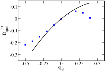
Figure 9: (Color online) Interplay between the $s$-wave interaction and the spin-orbit coupling term for the ground state for one atom with and one atom without spin-orbit coupling (case 1a; $\eta=1$). The solid line and squares show the quantity $D_{q_{\text{rel}}}^{(4)}$ that characterizes the fourth-order perturbation theory shift as a function of $q_{\text{rel}}$. The solid line shows the expansion around $q_{\text{rel}}=0$ [see Eq. (52)]. The squares show the full numerically determined values.

Figure 10 compares the perturbative prediction (solid line) with the full numerical energy obtained using the basis set expansion approach discussed in the Appendix for $1/a_{\text{aa}}=0$ and $\eta=1$. Circles show $\Delta E_{\text{gr}}^{\text{num}}$, see Eq. (35), as a function of $(k_{\text{so}}a_{\text{ho}})^{4}$. The solid line in Fig. 10 shows the scaled perturbative energy shift $D_{q_{\text{rel}}}^{(4)}(k_{\text{so}}a_{\text{ho}})^{4}$. The agreement is excellent for $(k_{\text{so}}a_{\text{ho}})^{4}\lesssim 0.004$ or $k_{\text{so}}a_{\text{ho}}\lesssim 0.25$.

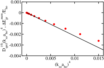
Figure 10: (Color online) Interplay between the $s$-wave interaction and the spin-orbit coupling term for the ground state for one atom with and one atom without spin-orbit coupling (case 1a with $1/a_{\text{aa}}=0$ and $\eta=1$). The solid line shows the quantity $D_{q_{\text{rel}}}^{(4)}(k_{\text{so}}a_{\text{ho}})^{4}$ for $q_{\text{rel}}=-1/2$ as a function of $(k_{\text{so}}a_{\text{ho}})^{4}$. Circles show the quantity $\Delta E_{\text{gr}}^{\text{num}}/E_{\text{ho}}$, see Eq. (35).

If we allow for different scattering lengths, i.e., if we set $a_{\uparrow}=a_{\text{aa}}$ and $a_{\downarrow}=\eta a_{\text{aa}}$, and assume $\eta\neq 1$ (case 1b), then the two states $\Psi_{q_{\text{aa}},1/2}^{(0)}$ and $\Psi_{q_{\eta\text{aa}},-1/2}^{(0)}$, which have—as before—$N_{\text{cm}}=M_{\text{cm}}=K_{\text{cm}}=l_{\text{rel}}=m_{\text{rel}}=0$, have different energies. Here, $q_{\text{aa}}$ and $q_{\eta\text{aa}}$ are the non-integer quantum numbers that solve the transcendental equation [Eq. (41)] for the states of interest with $a_{\text{aa}}$ and $\eta a_{\text{aa}}$, respectively. In what follows, we assume that $\Psi_{q_{\text{aa}},1/2}^{(0)}$ and $\Psi_{q_{\eta\text{aa}},-1/2}^{(0)}$ are not degenerate with any of the other unperturbed eigenstates with the same $M_{J}$ quantum number. In second-order perturbation theory, the energy shifts, which are determined by terms that contain two $V_{\text{so}}^{\text{cm},1}$’s, depend on $q_{\text{aa}}$ and $q_{\eta\text{aa}}$. Combining all second-order perturbation theory contributions, we find that the energy shift of the unperturbed state $\Psi_{q_{\text{aa}},1/2}^{(0)}$ is given by

$$\Delta E^{(\text{so},2)}_{M_{J}=1/2}=(-1+D_{q_{\text{aa}},q_{\eta\text{aa}}}^{(2)})(k_{\text{so}}a_{\text{ho}})^{2}E_{\text{ho}},$$ (53)

where

$$D_{q_{\text{aa}},q_{\eta\text{aa}}}^{(2)}=\frac{1}{2}+\frac{1}{2}\sum_{q_{\text{rel}}}\frac{(\sum_{j=0}^{\infty}C_{j}^{q_{\text{aa}}}C_{j}^{q_{\text{rel}}})^{2}}{2q_{\text{aa}}-(2q_{\text{rel}}+1)}$$ (54)

and $q_{\text{rel}}$ runs through all non-integer quantum numbers that solve the transcendental equation for $\eta a_{\text{aa}}$. For $\eta=1$, $D_{q_{\text{aa}},q_{\eta\text{aa}}}^{(2)}$ vanishes and Eq. (53) reduces to Eq. (50). In the weakly-interacting regime, i.e., for small $|a_{\text{aa}}|/a_{\text{ho}}$ and $|\eta a_{\text{aa}}|/a_{\text{ho}}$ ($q_{\text{aa}}$ and $q_{\eta\text{aa}}$ near zero), Eq. (54) reduces to

$$D_{q_{\text{aa}},q_{\eta\text{aa}}}^{(2)}=\left(-\frac{1}{2}-\frac{2-\log 4}{\sqrt{2\pi}}\frac{a_{\text{aa}}}{a_{\text{ho}}}+\cdots\right)\times$$

$$\left(1-\eta\right)\frac{E_{\text{scatt}}}{E_{\text{ho}}}.$$ (55)

The first term in large round brackets agrees with the second term in square brackets in Eq. (III.2).

To obtain the energy shift $\Delta E^{(\text{so},2)}_{M_{J}=-1/2}$ of the unperturbed state $\Psi_{q_{\eta\text{aa}},-1/2}^{(0)}$, $D_{q_{\text{aa}},q_{\eta\text{aa}}}^{(2)}$ needs to be replaced by $D_{q_{\eta\text{aa}},q_{\text{aa}}}^{(2)}$ in Eq. (53), $q_{\text{aa}}$ needs to be replaced by $q_{\eta\text{aa}}$ in Eq. (54), and $q_{\text{rel}}$ needs to run through all non-integer quantum numbers that solve the transcendental equation for $a_{\text{aa}}$. In the weakly-interacting limit ($q_{\eta\text{aa}}$ and $q_{\text{aa}}$ near zero), $D_{q_{\eta\text{aa}},q_{\text{aa}}}^{(2)}$ reduces to Eq. (IV.2) with $a_{\text{aa}}$ replaced by $\eta a_{\text{aa}}$ and $1-\eta$ replaced by $\eta-1$. For $\eta\neq 1$ (case 1b), the third-order perturbation theory yields zero and the fourth-order treatment is not pursued here.

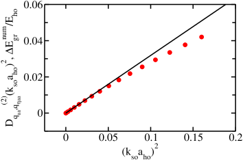
Figure 11: (Color online) Interplay between the $s$-wave interaction and the spin-orbit coupling term for the ground state for one atom with and one atom without spin-orbit coupling (case 1b with $1/a_{\text{aa}}=0$ and $\eta a_{\text{aa}}=0$). The solid line shows the quantity $D_{q_{\text{aa}},q_{\eta\text{aa}}}^{(2)}(k_{\text{so}}a_{\text{ho}})^{2}$ for $q_{\text{aa}}=-1/2$ and $q_{\eta\text{aa}}=0$ as a function of $(k_{\text{so}}a_{\text{ho}})^{2}$. Circles show the quantity $\Delta E_{\text{gr}}^{\text{num}}/E_{\text{ho}}$, see Eq. (35).

As an example, Fig. 11 compares the perturbative prediction with the full numerical energy obtained using the basis set expansion approach discussed in the Appendix for $1/a_{\text{aa}}=0$ and $\eta a_{\text{aa}}=0$ (case 1b). Circles show $\Delta E_{\text{gr}}^{\text{num}}/E_{\text{ho}}$, see Eq. (35), as a function of $(k_{\text{so}}a_{\text{ho}})^{2}$ while the solid line shows the scaled perturbative energy shift $D_{q_{\text{aa}},q_{\eta\text{aa}}}^{(2)}(k_{\text{so}}a_{\text{ho}})^{2}$. The agreement is excellent for $(k_{\text{so}}a_{\text{ho}})^{2}\lesssim 0.05$. Figure 11 shows that the interplay between the spin-orbit coupling term and the $s$-wave interaction accounts for approximately 0.04$E_{\text{ho}}$ of the energy for $(k_{\text{so}}a_{\text{ho}})^{2}=0.16$. This is a sizable effect that should be measurable with present-day technology.

To illustrate the behavior of the quantity $D_{q_{\text{aa}},q_{\eta\text{aa}}}^{(2)}$, Eq. (54), for other $q_{\text{aa}}$ and $q_{\eta\text{aa}}$ combinations, squares in Figs. 12(a)-12(d) show $D_{q_{\text{aa}},q_{\eta\text{aa}}}^{(2)}$ for $q_{\eta\text{aa}}=-1/2,-0.3,0$ and $1/2$, respectively, as a function of $q_{\text{aa}}$. The solid line in Fig. 12(c) shows the expansion for small $|q_{\text{aa}}|$ and $|q_{\eta\text{aa}}|$ [see Eq. (IV.2)]. Interestingly, the expansion provides a good description of the energy shift over a fairly large range of $q_{\text{aa}}$ values. For $q_{\text{aa}}<q_{\eta\text{aa}}$, the interplay between the spin-orbit coupling term and $s$-wave interaction leads to an increase of the energy. For $q_{\text{aa}}=q_{\eta\text{aa}}$ [$q_{\text{aa}}=-0.5,-0.3,0$ and $0.5$ in Figs. 12(a)-12(d), respectively], $D_{q_{\text{aa}},q_{\eta\text{aa}}}^{(2)}$ vanishes. For $q_{\eta\text{aa}}<q_{\text{aa}}<q_{\eta\text{aa}}+1/2$, the interplay between the spin-orbit coupling term and the $s$-wave interaction leads to a decrease of the energy. The behavior of $D_{q_{\text{aa}},q_{\eta\text{aa}}}^{(2)}$ in the vicinity of the hashed regions is discussed in the next section.

The key points of this section are:

• For $a_{\uparrow}=a_{\downarrow}$ ($\eta=1$), the leading-order energy shift of the ground state that reflects the interplay between the spin-orbit coupling and the $s$-wave interaction is proportional to $(k_{\text{so}})^{4}$ for all scattering lengths.

• For $a_{\uparrow}\neq a_{\downarrow}$ ($\eta\neq 1$), the leading-order energy shift of the ground state that reflects the interplay between the spin-orbit coupling and the $s$-wave interaction is, in general, proportional to $(k_{\text{so}})^{2}$ for all scattering lengths.

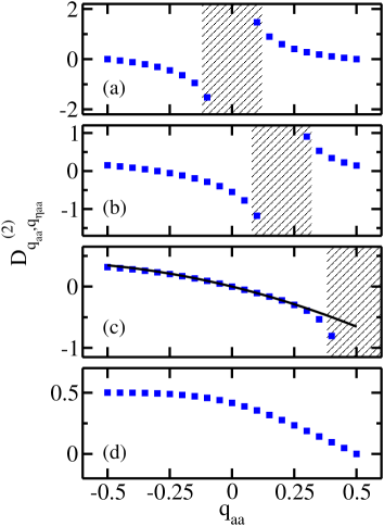
Figure 12: (Color online) Interplay between the $s$-wave interaction and the spin-orbit coupling term for one atom with and one atom without spin-orbit coupling (case 1b). The squares show the numerically calculated quantity $D_{q_{\text{aa}},q_{\eta\text{aa}}}^{(2)}$ [see Eq. (54)] that characterizes the second-order perturbation theory shift as a function of $q_{\text{aa}}$ for (a) $q_{\eta\text{aa}}=-1/2$, (b) $q_{\eta\text{aa}}=-0.3$, (c) $q_{\eta\text{aa}}=0$ and (d) $q_{\eta\text{aa}}=1/2$. The solid line in panel (c) shows the expansion for small $|q_{\text{aa}}|$ and $|q_{\eta\text{aa}}|$ [see Eq. (IV.2)]. The hashed regions in panels (a)-(c) show the parameter range where the non-degenerate perturbation theory treatment breaks down.

IV.3 Perturbative treatment of $V_{\text{so}}(\vec{r}_{1})$: Near-degenerate regime

To understand the behavior of $D_{q_{\text{aa}},q_{\eta\text{aa}}}^{(2)}$ near the hashed regions in Figs. 12(a)-12(c), it is important to recall that the derivation assumed that the states $\Psi_{q_{\text{aa}},1/2}^{(0)}$ and $\Psi_{q_{\eta\text{aa}},-1/2}^{(0)}$ are not degenerate with any other unperturbed eigenstates with the same $M_{J}$ quantum number. To understand the implications, we consider the situation where the unperturbed energy equals $(2q_{\text{aa}}+3)\hbar\omega\leq 4\hbar\omega$. In this case, the $\Psi_{q_{\text{aa}},1/2}^{(0)}$ state with $N_{\text{cm}}=M_{\text{cm}}=K_{\text{cm}}=l_{\text{rel}}=m_{\text{rel}}=0$ ($M_{J}=1/2$), referred to as state 1 in the following, is degenerate with the $M_{J}=1/2$ state with quantum numbers $(q_{\eta\text{aa}},l_{\text{rel}},m_{\text{rel}},N_{\text{cm}},M_{\text{cm}},K_{\text{cm}},m_{s})=(q_{\text{aa}}-1/2,0,0,0,1,0,-1/2)$, referred to as state 2. This degeneracy can be understood as follows. Since the relative energy is equal to $(2q_{\text{aa}}+3/2)\hbar\omega$ and $(2q_{\text{aa}}+1/2)\hbar\omega$ for states 1 and 2, respectively, the unperturbed two-body energies are degenerate if state 2 contains one “extra” quantum of energy in the center of mass degrees of freedom. Putting this extra quantum in the $M_{\text{cm}}$ quantum number (as opposed to $K_{\text{cm}}$) introduces a coupling between states 1 and 2 if the spin-orbit coupling term is turned on. In this case, the quantity $D_{q_{\text{aa}},q_{\eta\text{aa}}}^{(2)}$ does not provide a faithful description of the energy spectrum for $q_{\text{aa}}\approx q_{\eta\text{aa}}+1/2$, i.e., for $q_{\text{aa}}\approx 0,0.2$ and $1/2$ in Figs. 12(a)-12(c). As discussed in the following, the coupling between states 1 and 2 leads to an enhancement of the interplay between the spin-orbit coupling term and the $s$-wave interaction.

To determine the energy spectrum in the regime where states 1 and 2 have (near-)degenerate energies, we employ first-order near-degenerate perturbation theory baym . We define $\Delta$ through $q_{\text{aa}}=q_{\eta\text{aa}}+1/2+\Delta$ and assume $|\Delta|\ll 1$. We first diagonalize the Hamiltonian $H_{\text{soc,a}}$ in the Hilbert space spanned by states 1 and 2. The diagonal matrix elements are $(2q_{\text{aa}}+3)E_{\text{ho}}$ and $(2q_{\eta\text{aa}}+4)E_{\text{ho}}$ while the off-diagonal elements are $C_{q_{\text{aa}},q_{\eta\text{aa}}}^{(2)}k_{\text{so}}a_{\text{ho}}E_{\text{ho}}/\sqrt{2}$, where

$$C_{q_{\text{aa}},q_{\eta\text{aa}}}^{(2)}=\sum_{j=0}^{\infty}C_{j}^{q_{\text{aa}}}C_{j}^{q_{\eta\text{aa}}}$$ (56)

and the $C_{j}$’s are defined through Eq. (45). The resulting first-order energies are

$$E/E_{\text{ho}}=2q_{\text{aa}}+3-\Delta\pm$$

$$\frac{1}{2}\sqrt{4\Delta^{2}+2(C_{q_{\text{aa}},q_{\eta\text{aa}}}^{(2)})^{2}(k_{\text{so}}a_{\text{ho}})^{2}}.$$ (57)

The second-order treatment then yields additional shifts proportional to $(k_{\text{so}}a_{\text{ho}})^{2}$.

In the regime where the energy difference between states 1 and 2 is much smaller than the coupling between the two states ($|\Delta|\ll C_{q_{\text{aa}},q_{\eta\text{aa}}}^{(2)}k_{\text{so}}a_{\text{ho}}/\sqrt{2}$), we Taylor expand Eq. (57) around $\sqrt{2}\Delta/(C_{q_{\text{aa}},q_{\eta\text{aa}}}^{(2)}k_{\text{so}}a_{\text{ho}})=0$,

$$E/E_{\text{ho}}=2q_{\text{aa}}+3-\Delta\pm\frac{1}{\sqrt{2}}C_{q_{\text{aa}},q_{\eta\text{aa}}}^{(2)}k_{\text{so}}a_{\text{ho}}\times$$

$$\bigg{[}1+\frac{\Delta^{2}}{(C_{q_{\text{aa}},q_{\eta\text{aa}}}^{(2)})^{2}(k_{\text{so}}a_{\text{ho}})^{2}}+\cdots\bigg{]}.$$ (58)

For $\Delta=0$, Eq. (IV.3) reduces to the result obtained using degenerate perturbation theory. Equation (IV.3) shows that the interplay between the $s$-wave interaction and the spin-orbit coupling term leads to an energy shift proportional to $k_{\text{so}}a_{\text{ho}}$. In the regime where the energy difference between states 1 and 2 is much greater than the coupling ($C_{q_{\text{aa}},q_{\eta\text{aa}}}^{(2)}k_{\text{so}}a_{\text{ho}}/\sqrt{2}\ll|\Delta|$), we Taylor expand Eq. (57) around $C_{q_{\text{aa}},q_{\eta\text{aa}}}^{(2)}k_{\text{so}}a_{\text{ho}}/(\sqrt{2}\Delta)=0$,

$$E/E_{\text{ho}}=2q_{\text{aa}}+3-\Delta\pm\Delta\times$$

$$\bigg{[}1+\frac{(C_{q_{\text{aa}},q_{\eta\text{aa}}}^{(2)})^{2}(k_{\text{so}}a_{\text{ho}})^{2}}{4\Delta^{2}}+\cdots\bigg{]}.$$ (59)

The eigenstates corresponding to Eq. (IV.3) are approximately given by states 1 ($+$ sign) and 2 ($-$ sign), respectively. If we include the second-order energy shift, we recover our non-degenerate perturbation theory results given in Eqs. (53) and (54).

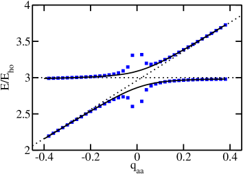
Figure 13: (Color online) Near-degenerate perturbation theory result for one atom with and one atom without spin-orbit coupling (case 1b with $q_{\eta\text{aa}}=-1/2$ and $k_{\text{so}}a_{\text{ho}}=0.2$). Dotted lines show the scaled energies $(E_{\text{gr}}^{s-\text{wave}}+E_{\text{gr}}^{\text{so}})/E_{\text{ho}}-3$ for the two $M_{J}=1/2$ states (see text) excluding the energy due to the interplay between the spin-orbit coupling term and the $s$-wave interaction. Solid lines show the energies predicted by the near-degenerate perturbation theory treatment up to second order. For comparison, squares show the energies predicted by non-degenerate perturbation theory [see Eq. (53) for the $M_{\text{cm}}=0$ state].

Figure 13 exemplarily illustrates the results of the near-degenerate perturbation theory treatment for $k_{\text{so}}a_{\text{ho}}=0.2$, $q_{\eta\text{aa}}=-1/2$ and varying $q_{\text{aa}}$ [this corresponds to the hashed region in Fig. 12(a)]. The dotted lines show the scaled energies $(E_{\text{gr}}^{s-\text{wave}}+E_{\text{gr}}^{\text{so}})/E_{\text{ho}}-3=2q_{\text{aa}}+3-(k_{\text{so}}a_{\text{ho}})^{2}$ and $3$, i.e., the energies of the system excluding the interplay between the spin-orbit coupling term and the $s$-wave interaction. The solid lines show the energies predicted by the near-degenerate perturbation theory treatment, including the first-order energies [see Eq. (57)] and the second-order energy shifts [not given in Eq. (57)]. For $q_{\text{aa}}=0$, the first-order energies reduce to $(3\pm\sqrt{1/\pi}k_{\text{so}}a_{\text{ho}})E_{\text{ho}}$. The term proportional to $k_{\text{so}}a_{\text{ho}}$ reflects the interplay between the spin-orbit coupling term and the $s$-wave interaction. As can be seen in Fig. 13, the interplay turns the sharp crossing (see dotted lines) into an avoided crossing (solid lines), with the energy splitting governed by $k_{\text{so}}$. The energy splitting for $q_{\text{aa}}=0$ is roughly $0.2E_{\text{ho}}$. This shift is much larger than the energy shifts introduced by the interplay between the spin-orbit coupling term and the $s$-wave interaction for non-degenerate states. This indicates that the interplay can, for certain parameter combinations, notably modify the energy spectrum even for relatively small $|k_{\text{so}}|$. For comparison, the squares show the second-order non-degenerate perturbation theory energies. The energy shift of state 1 is given in Eq. (53) [see also Fig. 12(a)] and the energy shift of state 2 has been calculated following a similar approach.

We note that there exist two other states with quantum numbers $(q_{\eta\text{aa}},l_{\text{rel}},m_{\text{rel}},N_{\text{cm}},M_{\text{cm}},K_{\text{cm}},m_{s})=(q_{\text{aa}}-1/2,0,0,0,-1,0,-1/2)$ and $(q_{\eta\text{aa}},l_{\text{rel}},m_{\text{rel}},N_{\text{cm}},M_{\text{cm}},K_{\text{cm}},m_{s})=(q_{\text{aa}}-1/2,0,0,0,0,1,-1/2)$ that have an energy of $(2q_{\text{aa}}+3)\hbar\omega$. However, since these states have $M_{J}=-3/2$ and $-1/2$, they do not couple to the $M_{J}=1/2$ states discussed in Eqs. (56)-(IV.3) and Fig. 13. The $M_{J}=-3/2$ and $-1/2$ states can be treated using second-order non-degenerate perturbation theory. In fact, the energy shift of the $M_{J}=-1/2$ state is given in Eq. (53). To get the energy shift of the $M_{J}=-3/2$ state, the $-1$ in Eq. (53) needs to be replaced by $-3/2$ and $D_{q_{\text{aa}},q_{\eta\text{aa}}}^{(2)}$ needs to be multiplied by 2. The energy shifts of these two states are proportional to $(k_{\text{so}}a_{\text{ho}})^{2}$ and their scaled energies would be indistinguishable from a horizontal line on the scale of Fig. 13.

The near-degenerate perturbation theory treatment can be applied to other parameter combinations for which degeneracies exist. As a second example, we return to the system with $\eta=1$ (case 1a). As stated earlier, Eq. (51) does not apply when $q_{\text{rel}}=1/2$ and $l_{\text{rel}}=m_{\text{rel}}=N_{\text{cm}}=M_{\text{cm}}=K_{\text{cm}}=0$, i.e., when the two-body energy of the unperturbed system equals $4\hbar\omega$. In this case, the system supports six degenerate $M_{J}=1/2$ states. We find that these states do not couple at first- and second-order perturbation theory. However, the second-order treatment yields energy shifts proportional to $-(k_{\text{so}}a_{\text{ho}})^{2}$ and $-(k_{\text{so}}a_{\text{ho}})^{2}/2$, thereby dividing the six states into two smaller degenerate manifolds. Treating these two manifolds separately, neither of the states acquires a third-order shift. We notice, however, that the states of these different manifolds are, due to the shifts proportional to $-(k_{\text{so}}a_{\text{ho}})^{2}$, degenerate at an energy less than $4\hbar\omega$ (and a $q_{\text{rel}}$ value slightly larger than $1/2$). Treating these new crossing points, we find energy shifts proportional to $k_{\text{so}}a_{\text{ho}}$ and avoided crossings governed by $(k_{\text{so}}a_{\text{ho}})^{3}$.

The discussion above shows that the perturbative treatment of (avoided) crossings, induced by the interplay between the spin-orbit coupling term and the $s$-wave interaction, requires great care. For the examples investigated, we find that the interplay between the spin-orbit coupling term and the $s$-wave interaction gives rise to leading-order energy shifts proportional to odd powers in $k_{\text{so}}a_{\text{ho}}$ in the vicinity of (avoided) crossings and to leading-order energy shifts proportional to even powers in $k_{\text{so}}a_{\text{ho}}$ away from (avoided) crossings. We expect that the avoided crossings, introduced by the interplay between the spin-orbit coupling term and the $s$-wave interaction, have an appreciable effect on the second-order virial coefficient and related observables.

The key point of this section is:

• The interplay between the spin-orbit coupling term and the $s$-wave interaction can, if the energy levels of unperturbed states cross, induce avoided crossings whose leading-order energy splitting is proportional to $k_{\text{so}}$.

IV.4 Perturbative treatment of $V_{\text{so}}(\vec{r}_{1})+V_{\text{so}}(\vec{r}_{2})$: Two particles with spin-orbit coupling

This section considers two particles with spin-orbit coupling. As in Sec. IV.2, we rewrite the spin-orbit coupling terms in terms of the relative and center of mass coordinates,

$$V_{\text{so}}(\vec{r}_{1})+V_{\text{so}}(\vec{r}_{2})=V_{\text{so}}^{\text{rel},1}(\vec{r}_{12})+V_{\text{so}}^{\text{cm},1}(\vec{R}_{12})$$

$$-V_{\text{so}}^{\text{rel},2}(\vec{r}_{12})+V_{\text{so}}^{\text{cm},2}(\vec{R}_{12}).$$ (60)

We assume $\omega_{x}=\omega_{y}=\omega_{z}$ and focus on the regime where center of mass excitations are absent and where $l_{\text{rel}}=m_{\text{rel}}=0$. As in Sec. IV.2, we account for the $s$-wave interaction non-perturbatively.

We start by considering case 2d, i.e., we consider the case with $\zeta,\eta\neq 1$ and $\zeta\neq\eta$, and determine the perturbative shifts of the states $\Psi_{1/2,1/2}^{(0)}=\psi_{0,0,0}^{\text{cm}}\psi_{q_{\text{aa}},0,0}^{\text{rel}}|\uparrow\rangle_{1}|\uparrow\rangle_{2}$, $\Psi_{-1/2,-1/2}^{(0)}=\psi_{0,0,0}^{\text{cm}}\psi_{q_{\zeta\text{aa}},0,0}^{\text{rel}}|\downarrow\rangle_{1}|\downarrow\rangle_{2}$, $\Psi_{1/2,-1/2}^{(0)}=\psi_{0,0,0}^{\text{cm}}\psi_{q_{\eta\text{aa}},0,0}^{\text{rel}}|\uparrow\rangle_{1}|\downarrow\rangle_{2}$ and $\Psi_{-1/2,1/2}^{(0)}=\psi_{0,0,0}^{\text{cm}}\psi_{q_{\eta\text{aa}},0,0}^{\text{rel}}|\downarrow\rangle_{1}\uparrow\rangle_{2}$ with $M_{J}=1,-1,0$ and $0$, respectively. Here $q_{\text{aa}}$, $q_{\zeta\text{aa}}$ and $q_{\eta\text{aa}}$ are obtained by solving the transcendental equation, Eq. (41), for $a_{\text{aa}}$, $\zeta a_{\text{aa}}$ and $\eta a_{\text{aa}}$, respectively.

We assume that $\Psi_{1/2,1/2}^{(0)}$ and $\Psi_{-1/2,-1/2}^{(0)}$ are not degenerate with any other states with the same $M_{J}$. Second-order non-degenerate perturbation theory then yields

$$\Delta E^{(\text{so},2)}_{M_{J}=1(S)}=2(-1+D_{q_{\text{aa}},q_{\eta\text{aa}}}^{(2)})(k_{\text{so}}a_{\text{ho}})^{2}E_{\text{ho}}$$ (61)

for $M_{J}=1$. The upper left arrow in Fig. 14 schematically illustrates how the $M_{J}=1$ state couples to the $M_{J}=0$ states. The energy shift $\Delta E^{(\text{so},2)}_{M_{J}=-1(S)}$ is given by Eq. (61) with $q_{\text{aa}}$ replaced by $q_{\zeta\text{aa}}$. The quantities $D_{q_{\text{aa}},q_{\eta\text{aa}}}^{(2)}$ and $D_{q_{\zeta\text{aa}},q_{\eta\text{aa}}}^{(2)}$ are defined in Eq. (54) and shown in Fig. 12 for different $q$ combinations. The states $\Psi_{1/2,-1/2}^{(0)}$ and $\Psi_{-1/2,1/2}^{(0)}$ are degenerate. Assuming no additional degeneracies with other $M_{J}=0$ states exist, degenerate perturbation theory yields the second-order perturbation shifts

$$\Delta E^{(\text{so},2)}_{M_{J}=0(S)}=2(-1+D_{q_{\eta\text{aa}},q_{\text{aa}}}^{(2)}+$$

$$D_{q_{\eta\text{aa}},q_{\zeta\text{aa}}}^{(2)})(k_{\text{so}}a_{\text{ho}})^{2}E_{\text{ho}}$$ (62)

and

$$\Delta E^{(\text{so},2)}_{M_{J}=0(A)}=-2(k_{\text{so}}a_{\text{ho}})^{2}E_{\text{ho}},$$ (63)

where $D_{q_{\eta\text{aa}},q_{\text{aa}}}^{(2)}$ and $D_{q_{\eta\text{aa}},q_{\zeta\text{aa}}}^{(2)}$ are defined in Eq. (54). The eigenstates corresponding to Eqs. (IV.4) and (63) are respectively symmetric and anti-symmetric under the exchange of particles 1 and 2. The lower arrows in Fig. 14 schematically illustrate the structure of Eq. (IV.4).

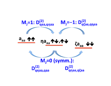
Figure 14: (Color online) Schematic illustration of Eqs. (61) and (IV.4). The horizontal lines show the four unperturbed states under consideration, labeled by their single particle spins and scattering lengths (since the unperturbed states $\Psi_{1/2,-1/2}^{(0)}$ and $\Psi_{-1/2,1/2}^{(0)}$ are degenerate, they are represented by a single line); the horizontal lines are vertically offset to reflect the fact that they have different energies. According to Eq. (61), the coupling of the $M_{J}=1$ ($M_{J}=-1$) state to the $M_{J}=0$ states is described by $D_{q_{\text{aa}},q_{\eta\text{aa}}}^{(2)}$ ($D_{q_{\zeta\text{aa}},q_{\eta\text{aa}}}^{(2)}$). According to Eq. (IV.4), the coupling of the symmetric $M_{J}=0$ state to the $M_{J}=1$ and $-1$ states is described by $D_{q_{\eta\text{aa}},q_{\text{aa}}}^{(2)}$ and $D_{q_{\eta\text{aa}},q_{\zeta\text{aa}}}^{(2)}$, respectively.

In the weakly-interacting regime (all $|q|$’s much smaller than 1), the $D^{(2)}$ coefficient can be expanded [see Eq. (IV.2)]. The resulting energy shifts proportional to $a_{\text{aa}}$ agree with those derived in Sec. III.3. The treatment above breaks down when additional degeneracies exist. In this case, near-degenerate perturbation theory provides, in much the same way as discussed in Sec. IV.3, a reliable description of avoided crossings.

We find that Eqs. (61)-(63) hold in the limits that $\zeta$ or $\eta$ or both go to 1. For $\zeta=1$ and $\eta\neq 1$ (case 2b), the states $\Psi_{1/2,1/2}^{(0)}$ and $\Psi_{-1/2,-1/2}^{(0)}$ are degenerate and have the same perturbation shift. For $\zeta\neq 1$ and $\eta=1$ (case 2c), $D_{q_{\text{aa}},q_{\eta\text{aa}}}^{(2)}$ vanishes. The energy shift of the $M_{J}=1$ state contains no term proportional to $(k_{\text{so}}a_{\text{ho}})^{2}$ while the energy shifts of the $M_{J}=-1$ and $M_{J}=0$ states with bosonic exchange symmetry contain shifts proportional to $(k_{\text{so}}a_{\text{ho}})^{2}$. In the limit that $\zeta=1$ and $\eta=1$ (case 2a), $D_{q_{\text{aa}},q_{\eta\text{aa}}}^{(2)}$, $D_{q_{\zeta\text{aa}},q_{\eta\text{aa}}}^{(2)}$, $D_{q_{\eta\text{aa}},q_{\text{aa}}}^{(2)}$ and $D_{q_{\eta\text{aa}},q_{\zeta\text{aa}}}^{(2)}$ vanish. In this case, the interaction does not break the degeneracy of the four unperturbed states and the energy shift contains no term proportional to $(k_{\text{so}}a_{\text{ho}})^{2}$.

Figure 15 compares the perturbative prediction (solid line) with our numerical basis set expansion results (circles) for case 2b. Figure 15(a) shows the case where $1/a_{\text{aa}}=0$, $\zeta=1$ and $\eta a_{\text{aa}}=0$. The lowest energy state is two-fold degenerate ($|M_{J}|=1$) and possesses bosonic exchange symmetry. The leading-order energy shift that reflects the interplay between the spin-orbit coupling term and the $s$-wave interaction is proportional to $(k_{\text{so}})^{2}$ [see Eq. (61)]. Figure 15(b) shows the case where $a_{\text{aa}}=0$, $\zeta=1$ and $1/(\eta a_{\text{aa}})=0$. The lowest energy state possesses fermionic exchange symmetry. According to Eq. (63), the interplay between the spin-orbit coupling term and the $s$-wave interaction does not give rise to an energy shift proportional to $(k_{\text{so}})^{2}$. This is confirmed by our numerical results (circles).

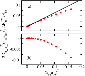
Figure 15: (Color online) Interplay between the $s$-wave interaction and the spin-orbit coupling term for the ground state manifold for two atoms with spin-orbit coupling. (a) The solid line shows the expression $2D_{q_{\text{aa}},q_{\eta\text{aa}}}^{(2)}(k_{\text{so}}a_{\text{ho}})^{2}$, see Eq. (61), for the lowest energy state as a function of $(k_{\text{so}}a_{\text{ho}})^{2}$ for case 2b with $1/a_{\text{aa}}=0$, $\zeta=1$ and $\eta a_{\text{aa}}=0$. For comparison, the circles show the quantity $\Delta E_{\text{gr}}^{\text{num}}/|E_{\text{scatt}}|$, see Eq. (35). (b) The circles show the quantity $\Delta E_{\text{gr}}^{\text{num}}/|E_{\text{scatt}}|$ for case 2b with $a_{\text{aa}}=0$, $\zeta=1$ and $1/(\eta a_{\text{aa}})=0$. The numerical data confirm the absence of a term proportional to $(k_{\text{so}}a_{\text{ho}})^{2}$, as predicted by Eq. (63).

The key points of this section are:

• For two identical bosons, the energy shift proportional to $(k_{\text{so}})^{2}$ is non-zero for the ground state for all scattering lengths unless $a_{\uparrow\uparrow}=a_{\downarrow\downarrow}=a_{\uparrow\downarrow}=a_{\downarrow\uparrow}$ $(\zeta=\eta=1)$ or, depending on the actual values of the scattering lengths, $a_{\uparrow\uparrow}=a_{\uparrow\downarrow}=a_{\downarrow\uparrow}$ $(\eta=1)$.

• For two identical fermions, the energy shift of the ground state due to the interplay between the spin-orbit coupling term and the $s$-wave interaction does not contain a term proportional to $(k_{\text{so}})^{2}$ for any scattering lengths.

V Conclusion

For two point particles under external spherically symmetric harmonic confinement with zero-range interaction, compact expressions for the eigenenergies and eigenfunctions were obtained in 1998 by Busch and coworkers busc98 . These solutions (and the two- and one-dimensional analogs) have played a crucial role in, to name a few examples, analyzing few-atom experiments esslinger05 ; esslinger06 ; jochim12 , guiding and benchmarking few-body calculations blume07 ; kestner07 ; vankolck07 , and interpreting the dynamics of many-body systems blume03 ; bohn13 . This paper determined portions of the energy spectrum of two $s$-wave interacting atoms under external spherically symmetric harmonic confinement with spin-orbit coupling of Rashba type. The spin-orbit coupling term introduces a new length scale as well as new internal degrees of freedom or pseudo-spin states for the point particles subject to the spin-orbit coupling. Our calculations consider, building on the seminal work by Busch and coworkers busc98 , two-atom systems with arbitrary $s$-wave scattering length and small spin-orbit coupling strength. We emphasize that the techniques developed in this work can be adapted for treating non-spherical traps, lower dimensional harmonic traps or different spin-orbit coupling terms. The treatment of anisotropic traps, e.g., would utilize the analytical solutions of Refs. calarco05 ; calarco06 .

We obtained a large number of analytical results for the small spin-orbit coupling strength regime. Both the small and large scattering length regime were considered. In the weakly-interacting regime, our results yield the leading-order mean-field shift. For pure $s$-wave interactions the leading-order mean-field shift of the trapped Bose gas is given by $N(N-1)E_{\text{scatt}}$. Our calculations show how this leading-order mean-field shift is modified in the presence of a weak spin-orbit coupling term of Rashba type. At which order the leading interplay between the spin-orbit coupling term and the $s$-wave interaction arises depends strongly on whether or not both particles feel the spin-orbit coupling as well as on the actual values of the scattering lengths. We discussed scenarios where the leading-order interplay between the spin-orbit coupling term and the $s$-wave interaction arises at order $k_{\text{so}}$, $k_{\text{so}}^{2}$, $k_{\text{so}}^{3}$ and $k_{\text{so}}^{4}$. A particularly strong interplay between the spin-orbit coupling term and the $s$-wave interaction was found in the vicinity of degeneracies, where the spin-orbit coupling term can turn sharp crossings into avoided crossings.

Many of our perturbative results were validated by a numerical basis set expansion approach for a wide range of $s$-wave scattering lengths. Although most of our analysis was performed for the spin-orbit coupling of Rashba type, the discussion in Sec. III.1 shows that at least some of our findings also apply to systems with a spin-orbit coupling term of a different functional form. For example, we found that, if only one of the particles feels the spin-orbit coupling and $a_{\uparrow}=a_{\downarrow}=a_{\text{aa}}$, the energy shift of the ground state does not contain a term proportional to $a_{\text{aa}}(k_{\text{so}})^{2}$. This result also holds for anisotropic spin-orbit coupling of Rashba type and a spin-orbit coupling term that only involves the $x$-component $p_{x}$ of the momentum.

Our analytical calculations employed a zero-range $s$-wave model potential. To account for finite-range effects, a momentum dependent term needs to be added. For the weakly-interacting trapped system, this yields an additional energy shift proportional to $r_{\text{eff}}a_{\text{aa}}^{2}$, where $r_{\text{eff}}$ is the effective range NJP2 . Our comparisons between the numerical and perturbative results accounted for first- and higher-order effective range corrections non-perturbatively by introducing the quantity $E_{\text{gr}}^{s-\text{wave}}$ in Eq. (35). In the weakly-interacting regime, we find that the leading-order interplay between the spin-orbit coupling term and the effective range scales as $r_{\text{eff}}a_{\text{aa}}^{2}k_{\text{so}}^{2}$ (or higher order) for the ground state. We estimate that this term, for $|k_{\text{so}}|a_{\text{ho}}>|a_{\text{aa}}|/a_{\text{ho}}$, is smaller than the terms that describe the interplay between the $s$-wave contact interaction and the spin-orbit coupling term considered in this paper.

It would be interesting to extend the perturbative and numerical calculations presented in this paper to more than two particles. In pure $s$-wave systems, effective three- and higher-body interactions have been shown to emerge NJP1 ; NJP2 . An intriguing question is how these effective few-body interactions depend on the spin-orbit coupling term. Another interesting question is how the thermodynamics of Bose and Fermi gases with spin-orbit coupling differs from the thermodynamics of Bose and Fermi gases without spin-orbit coupling. A first answer to this question can be obtained by looking at the virial equation of state up to second order in the fugacity ho04 . The virial equation of state depends on the second-order virial coefficient, which can be calculated if the complete energy spectrum of the trapped two particle system is known drummond09 . Thus, a natural extension of the present work is to push the two-particle calculations to higher energies and to larger spin-orbit coupling strengths. The large spin-orbit coupling regime has received a great deal of attention recently. In free space, the two-body binding energy has been calculated and analytic expressions applicable in weak and strong binding limits have been derived magarill06 ; shenoy11 ; galitski12 . It will be interesting to perform analogous calculations for the trapped two-particle system with large $|k_{\text{so}}|a_{\text{ho}}$.

VI Acknowledgements

DB gratefully acknowledges J. Shertzer for providing an efficient iterative generalized eigenvalue problem solver. XYY and DB acknowledge support by the National Science Foundation (NSF) through Grant No. PHY-1205443. SG acknowledges support through the Harvard Quantum Optics Center. This work was additionally supported by the NSF through a grant for the Institute for Theoretical Atomic, Molecular and Optical Physics at Harvard University and Smithsonian Astrophysical Observatory.

Appendix A Basis set expansion approach

To determine the eigenenergies of the two-particle system numerically, we expand the eigenstates in terms of basis functions that contain explicitly correlated Gaussians whose parameters are optimized semi-stochastically and solve the resulting generalized eigenvalue problem cgbook ; cgrmp . We first consider the situation where the first particle feels the spin-orbit coupling while the second particle does not. We write the eigenstate $\Psi_{\text{soc,a}}(\vec{r}_{1},\vec{r}_{2})$ of the Hamiltonian $H_{\text{soc,a}}$ [see Eq. (2)] with $V_{\text{2b}}^{\sigma}(\vec{r}_{12})=V_{\text{g}}^{\sigma}(\vec{r}_{12})$ as

$$\Psi_{\text{soc,a}}(\vec{r}_{1},\vec{r}_{2})=\psi_{\uparrow}(\vec{r}_{1},\vec{r}_{2})|\uparrow\rangle_{1}+\psi_{\downarrow}(\vec{r}_{1},\vec{r}_{2})|\downarrow\rangle_{1}$$ (64)

and expand $\psi_{\uparrow}$ and $\psi_{\downarrow}$ in terms of geminals $g_{j}$ cgbook ,

$$\psi_{\sigma}(\vec{r}_{1},\vec{r}_{2})=\sum_{j=1}^{N_{b}}c_{j}^{(\sigma)}g_{j}(\vec{R},\underline{A}^{(j)},\vec{s}^{(j)}),$$ (65)

where the $c_{j}^{(\sigma)}$ denote expansion coefficients and $N_{b}$ denotes the number of basis functions or geminals included in the expansion. The eigenstate of interest can be the ground state or an excited state. The vector $\vec{R}$ collectively denotes the spatial degrees of freedom, $\vec{R}=(\vec{r}_{1},\vec{r}_{2})$.

Each geminal $g_{j}$ is written in terms of a real and symmetric $2\times 2$ matrix $\underline{A}^{(j)}$ and a six-component vector $\vec{s}^{(j)}$, $\vec{s}^{(j)}=(s_{1}^{(j)},\cdots,s_{6}^{(j)})$:

$$g_{j}(\vec{R},\underline{A}^{(j)},\vec{s}^{(j)})=\exp\left[-\frac{1}{2}\vec{R}^{T}\underline{A}^{(j)}\vec{R}+(\vec{s}^{(j)})^{T}\vec{R}\right].$$ (66)

For concreteness, we write the argument of the exponential out explicitly; we have

$$(\vec{s}^{(j)})^{T}\vec{R}=s_{1}^{(j)}x_{1}+s_{2}^{(j)}y_{1}+\cdots+s_{6}^{(j)}z_{2}$$ (67)

and

$$\vec{R}^{T}\underline{A}^{(j)}\vec{R}=(A_{11}^{(j)}+A_{22}^{(j)})(\vec{r}_{1}^{2}+\vec{r}_{2}^{2})+$$

$$2A_{12}^{(j)}(x_{1}x_{2}+y_{1}y_{2}+z_{1}z_{2}),$$ (68)

where $A_{kl}^{(j)}$ denotes the $kl$’s element of the matrix $\underline{A}^{(j)}$. The geminals $g_{j}$ have neither a definite orbital angular momentum or projection quantum number nor a definite parity and are thus suited to describe the eigenstates of the two-particle system with spin-orbit coupling. A key characteristic of the geminals is that the Hamiltonian and overlap matrix elements reduce to compact analytical expressions cgbook if the atom-atom interaction is modeled by the Gaussian potential $V_{\text{g}}^{\sigma}$ [see Eq. (9)].

To construct the basis, we follow Ref. debraj12 . We start with just one basis function, i.e., we set $N_{b}=1$. We calculate the $2\times 2$ Hamiltonian and overlap matrices, and diagonalize the resulting eigenvalue problem. In general, the Hamiltonian and overlap matrices have dimension $(2N_{b})\times(2N_{b})$. The factor of $2$ has its origin in the two internal degrees of freedom (pseudo-spin states) of the first particle. To add a new basis function, we generate several thousand trial basis functions semi-stochastically, i.e., we choose the $A_{kl}^{(2)}$ and $s_{k}^{(2)}$ randomly from physically motivated preset “parameter value windows”, and select the basis function that lowers the energy of the state of interest the most. This procedure is repeated till the basis set has reached the desired size, i.e., till the energy of the state of interest is converged to the desired accuracy.

The above approach generalizes readily to the situation where both particles feel the spin-orbit coupling [see Eq. (3) for the Hamiltonian]. In this case, we write

$$\Psi_{\text{soc,soc}}(\vec{r}_{1},\vec{r}_{2})=$$

$$\psi_{\uparrow\uparrow}(\vec{r}_{1},\vec{r}_{2})|\uparrow\rangle_{1}|\uparrow\rangle_{2}+\psi_{\uparrow\downarrow}(\vec{r}_{1},\vec{r}_{2})|\uparrow\rangle_{1}|\downarrow\rangle_{2}+$$

$$\psi_{\downarrow\uparrow}(\vec{r}_{1},\vec{r}_{2})|\downarrow\rangle_{1}|\uparrow\rangle_{2}+\psi_{\downarrow\downarrow}(\vec{r}_{1},\vec{r}_{2})|\downarrow\rangle_{1}|\downarrow\rangle_{2}$$ (69)

and expand the $\psi_{\sigma\sigma^{\prime}}(\vec{r}_{1},\vec{r}_{2})$ in terms of geminals [Eq. (65) with $\sigma$ replaced by $\sigma\sigma^{\prime}$]. Since each particle has two internal degrees of freedom, the overlap and Hamiltonian matrices that define the generalized eigenvalue problem are $(4N_{b})\times(4N_{b})$-dimensional.

To validate our implementation, we performed several checks: (i) We set the atom-atom potential to zero and determine the eigenenergies for various $k_{\text{so}}$. We find that the ground state energy obtained by the numerical basis set expansion approach agrees, within the basis set extrapolation error, with the sum of the single-particle energies (see Sec. III.1 for the determination of the single-particle energies). (ii) We set $k_{\text{so}}=0$ and determine the eigenenergies for various depths of the Gaussian model potential. In these calculations, we fix $r_{0}$ at $r_{0}=0.02a_{\text{ho}}$. We find that the ground state energy obtained by the basis set expansion approach agrees, within the basis set extrapolation error, with the energies obtained by a highly accurate B-spline approach that separates the relative and center of mass degrees of freedom and takes advantage of the spherical symmetry of the system for $k_{\text{so}}=0$. We find that the basis set expansion approach describes the two-particle systems with $a_{\text{ho}}/a_{\sigma}\lesssim 2$ ($a_{\text{ho}}/a_{\sigma\sigma^{\prime}}\lesssim 2$) quite accurately. In Secs. III and IV, we compare the energies obtained by the basis set expansion approach with those obtained perturbatively in the small $|k_{\text{so}}|a_{\text{ho}}$ regime. Our calculations reveal a rich interplay between the atom-atom interaction and the spin-orbit coupling term. The basis set expansion calculations reported in Secs. III and IV use $N_{b}\approx 200-400$.

References

- (1) J. Dalibard, F. Gerbier, G. Juzeliūnas, and P. Öhberg, Rev. Mod. Phys. 83, 1523 (2011).
- (2) V. Galitski and I. B. Spielman, Nature 494, 49 (2013).
- (3) N. Goldman, G. Juzeliūnas, P. Öhberg, and I. B. Spielman, Preprint at arXiv:1308.6533.
- (4) H. Zhai, Int. J. Mod. Phys. B 26, 1230001 (2012).
- (5) Y.-J. Lin, K. Jiménez-García, and I. B. Spielman, Nature 471, 83 (2011).
- (6) P. Wang, Z.-Q. Yu, Z. Fu, J. Miao, L. Huang, S. Chai, H. Zhai, and J. Zhang, Phys. Rev. Lett. 109, 095301 (2012).
- (7) Z. Fu, L. Huang, Z. Meng, P. Wang, L. Zhang, S. Zhang, H. Zhai, P. Zhang, and J. Zhang, Preprint at arXiv:1306.4568.
- (8) R. A. Williams, M. C. Beeler, L. J. LeBlanc, K. Jiménez-García, and I. B. Spielman, Phys. Rev. Lett. 111, 095301 (2013).
- (9) C. Qu, C. Hamner, M. Gong, C. Zhang, and P. Engels, Phys. Rev. A 88, 021604(R) (2013).
- (10) A. Olson, S.-J. Wang, R. J. Niffenegger, C.-H. Li, C. H. Greene, and Y. P. Chen, Preprint at arXiv:1310.1818.
- (11) L. W. Cheuk, A. T. Sommer, Z. Hadzibabic, T. Yefsah, W. S. Bakr, and M. W. Zwierlein, Phys. Rev. Lett. 109, 095302 (2012).
- (12) C. Wu, I. Mondragon-Shem, and X.-F. Zhou, Chin. Phys. Lett. 28, 097102 (2011).
- (13) C. Wang, C. Gao, C. M. Jian, and H. Zhai, Phys. Rev. Lett. 105, 160403 (2010).
- (14) L. Jiang, X.-J. Liu, H. Hu, and H. Pu, Phys. Rev. A 84, 063618 (2011).
- (15) B. Ramachandhran, B. Opanchuk, X.-J. Liu, H. Pu, P. D. Drummond, and H. Hu, Phys. Rev. A 85, 023606 (2012).
- (16) T. D. Stanescu, B. Anderson, and V. Galitski, Phys. Rev. A 78, 023616 (2008).
- (17) M. Gong, S. Tewari, and C. Zhang, Phys. Rev. Lett. 107, 195303 (2011).
- (18) Z.-Q. Yu and H. Zhai, Phys. Rev. Lett. 107, 195305 (2011).
- (19) S. Gopalakrishnan, A. Lamacraft, and P. M. Goldbart, Phys. Rev. A 84, 061604(R) (2011).
- (20) T. Ozawa and G. Baym, Phys. Rev. A 85, 013612 (2012).
- (21) T. Ozawa and G. Baym, Phys. Rev. A 84, 043622 (2011).
- (22) R. A. Williams, L. J. LeBlanc, K. Jiménez-García, M. C. Beeler, A. R. Perry, W. D. Phillips, and I. B. Spielman, Science 335, 314 (2012).
- (23) P. Zhang, L. Zhang, and W. Zhang, Phys. Rev. A 86, 042707 (2012).
- (24) P. Zhang, L. Zhang, and Y. Deng, Phys. Rev. A 86, 053608 (2012).
- (25) L. Zhang, Y. Deng, and P. Zhang, Phys. Rev. A 87, 053626 (2013).
- (26) X. Cui, Phys. Rev. A 85, 022705 (2012).
- (27) H. Duan, L. You, and B. Gao, Phys. Rev. A 87, 052708 (2013).
- (28) F. Serwane, G. Zürn, T. Lompe, T. B. Ottenstein, A. N. Wenz, and S. Jochim, Science 332, 336 (2011).
- (29) S. Will, T. Best, U. Schneider, L. Hackermüller, D.-S. Lühmann, and I. Bloch, Nature 465, 197 (2010).
- (30) M. Studer, G. Salis, K. Ensslin, D. C. Driscoll, and A. C. Gossard, Phys. Rev. Lett. 103, 027201 (2009).
- (31) S. Chesi and G. F. Giuliani, Phys. Rev. B 83, 235308 (2011).
- (32) Y. Kanai, R. S. Deacon, S. Takahashi, A. Oiwa, K. Yoshida, K. Shibata, K. Hirakawa, Y. Tokura, and S. Tarucha, Nature Nanotechnology 6, 511 (2011).
- (33) M. Governale, Phys. Rev. Lett. 89, 206802 (2002).
- (34) T. Chakraborty and P. Pietiläinen, Phys. Rev. B 71, 113305 (2005).
- (35) E. Lipparini, M. Barranco, F. Malet, and M. Pi, Phys. Rev. B 79, 115310 (2009).
- (36) A. Cavalli, F. Malet, J. C. Cremon, and S. M. Reimann, Phys. Rev. B 84, 235117 (2011).
- (37) S. Nadj-Perge, S. M. Frolov, E. P. A. M. Bakkers, and L. P. Kouwenhoven, Nature 468, 1084 (2010).
- (38) T. Busch, B.-G. Englert, K. Rza̧żewski, and M. Wilkens, Found. Phys. 28, 549 (1998).
- (39) Y. A. Bychkov and E. I. Rashba, J. Phys. Chem. 17, 6039 (1984).
- (40) H. G. Reik, P. Lais, M. E. Stützle, and M. Doucha, J. Phys. A 87, 6327 (1987).
- (41) H. Tütüncüler, R. Koç, and E. Olğar, J. Phys. A 37, 11431 (2004).
- (42) C. Chin, R. Grimm, P. Julienne, and E. Tiesinga, Rev. Mod. Phys. 82, 1225 (2010).
- (43) C. R. Hamner, Ph.D. thesis, Washington State University, 2014.
- (44) H. A. Kramers, Proc. Amsterdam Acad. 33, 959 (1930).
- (45) M. J. Klein, Am. J. Phys. 20, 65 (1952).
- (46) O. V. Marchuov, A. G. Volosniev, D. V. Fedorov, A. S. Jensen, and N. T. Zinner, J. Phys. B 46, 134012 (2012).
- (47) P. R. Johnson, E. Tiesinga, J. V. Porto, and C. J. Williams, New J. Phys. 11, 093022 (2009).
- (48) P. R. Johnson, D. Blume, X. Y. Yin, W. F. Flynn, and E. Tiesinga, New J. Phys. 14, 053037 (2012).
- (49) As discussed in the text, the perturbation expression, Eq. (III.3), which corresponds to an anti-symmetric state, is independent of and . The calculations based on the basis set expansion approach use a Gaussian potential with the specified in the four scattering channels. The fact that the numerical results are well described by alone underlines the fact that the up-up and down-down channels are “turned off” by the anti-symmetry of the wave function.
- (50) K. M. Daily, X. Y. Yin, and D. Blume, Phys. Rev. A 85, 053614 (2012).
- (51) G. Baym. Lectures on Quantum Mechanics. Westview Press, Boulder (1969).
- (52) H. Moritz, T. Stöferle, K. Günter, M. Köhl, and T. Esslinger, Phys. Rev. Lett. 94, 210401 (2005).
- (53) T. Stöferle, H. Moritz, K. Günter, M. Köhl, and T. Esslinger, Phys. Rev. Lett. 96, 030401 (2006).
- (54) G. Zürn, F. Serwane, T. Lompe, A. N. Wenz, M. G. Ries, J. E. Bohn, and S. Jochim, Phys. Rev. Lett. 108, 075303 (2012).
- (55) J. von Stecher, C. H. Greene, and D. Blume, Phys. Rev. A 76, 053613 (2007).
- (56) J. P. Kestner and L.-M. Duan, Phys. Rev. A 76, 033611 (2007).
- (57) I. Stetcu, B. R. Barrett, U. van Kolck, and J. P. Vary, Phys. Rev. A 76, 063613 (2007).
- (58) B. Borca, D. Blume, and C. H. Greene, New J. Phys. 5, 111 (2003).
- (59) A. G. Sykes, J. P. Corson, J. P. D’Incao, A. P. Koller, C. H. Greene, A. M. Rey, K. R. A. Hazzard, and J. L. Bohn, Preprint at arXiv:1309.0828
- (60) Z. Idziaszek and T. Calarco, Phys. Rev. A 71, 050701(R) (2005).
- (61) Z. Idziaszek and T. Calarco, Phys. Rev. A 74, 022712 (2006).
- (62) T.-L. Ho and E. J. Mueller, Phy. Rev. Lett. 92, 160404 (2004).
- (63) X.-J. Liu, H. Hu, and P. D. Drummond, Phys. Rev. Lett. 102, 160401 (2009).
- (64) A. V. Chaplik and L. I. Magarill, Phys. Rev. Lett. 96, 126402 (2006).
- (65) J. P. Vyasanakere and V. B. Shenoy, Phys. Rev. B 83, 094515 (2011).
- (66) S. Takei, C.-H. Lin, B. M. Anderson, and V. Galitski, Phys. Rev. A 85, 023626 (2012).
- (67) Y. Suzuki and K. Varga. Stochastic Variational Approach to Quantum Mechanical Few-Body Problems. Springer Verlag, Berlin (1998).
- (68) J. Mitroy, S. Bubin, W. Horiuchi, Y. Suzuki, L. Adamowicz, W. Cencek, K. Szalewicz, J. Komasa, D. Blume, and K. Varga, Rev. Mod. Phys. 85, 693 (2013).
- (69) D. Rakshit, K. M. Daily, and D. Blume, Phys. Rev. A 85, 033634 (2012).