Linking Dynamic and Thermodynamic Properties of Cuprates; an ARPES study of (CaLa)(BaLa)₂Cu₃O_y

Abstract

We report angle-resolved photoemission spectroscopy (ARPES) on two families of high temperature superconductors (Ca_xLa_1-x)(Ba_1.75-x La _0.25+x)Cu₃O_y with $x=0.1$ ($T_{c}^{max}=56$ K) and $x=0.4$ ($T_{c}^{max}=82$ K). The Fermi surface (FS) is found to be independent of $x$ or $y$, and its size indicates extreme sample-surface overdoping. This universal FS allowes the comparison of dynamical properties between superconductors of similar structure and identical doping, but different $T_{c}^{max}$. We find that the high-energy ($\left|E\right|>50$ meV) nodal velocity in the $x=0.4$ family is higher than in the $x=0.1$ family. The implied correlation between $T_{c}^{max}$ and the hopping rate $t$ supports the notion of kinetic energy driven superconductivity in the cuprates. We also find that the antinodal gap is higher for the $x=0.4$ family.

The recent synthesis of charge compensated (Ca_xLa_1-x)(Ba_1.75-xLa_0.25+x)Cu₃O_y (CLBLCO) single crystals facilitates an investigation of the relationship between their dynamical properties, such as the electronic dispersion relation $E(\mathbf{k})$ and their thermodynamic property $T_{c}$, while applying subtle crystal structure changes Crystal . Since the valence of Ca and Ba is equal, $x$ has a minute effect on crystal structure but a large effect on $T_{c}$. Therefore, CLBLCO allows experiments where the correlations between $T_{c}$ and a single parameter are explored. Experiments of such nature can reveal the mechanism for cuprates’ superconductivity. In the present work, we measure the electron dispersion $E(\mathbf{k})$ of two extreme samples of CLBLCO crystals, using angle-resolved photoemission spectroscopy (ARPES), and look for correlations between properties of $E(\mathbf{k})$ and $T_{c}$. In particular, we focus on the nodal velocity. Previously, similar studies could only be done by comparing cuprates with very different structures and levels of disorder EdeggerPRL06 .

CLBLCO is similar to YBCO in crystal structure, but has no oxygen chain ordering and is tetragonal for all $x$ and $y$ Yaki99 . This simplifies the ARPES interpretation. While $x$ alters the calcium-to-barium ratio, the lanthanum content in the chemical formula remains constant. We define four CLBLCO ”families” as samples with different $x$, namely, $x=0.1,0.2,0.3,0.4$. The parameter $y$ signifies the oxygen level, which drives the system between different phases. By varying $x$ and $y$ in the chemical formula, one can generate phase diagrams that are similar in shape yet differ in the maximum of $T_{c}$, $T_{g}$, and $T_{N}$, and in the critical oxygen level at which the nature of the phase diagram changes. The phase diagram is presented in Fig. 1(a) AmitPRB10 . It is worth noting that the only structural properties that vary with $x$ or $y$ are the Cu-O-Cu buckling angle, bond length, and CuO₂ plane doping efficiency $K(x)$. The crystallographic parameters were measured with powder neutron diffraction OferPRB08 . The buckling angle decreases by $0.5$ degrees as $x$ increases between families. The bond length varies from $3.88$ Å for $x=0.4$ to $3.91~{}$Å at $x=0.1$. The doping efficiency is determined by in-plane ¹⁷O nuclear quadrupole resonance (NQR) AmitPRB10 . The variation in the number of holes on an oxygen $\Delta n_{p_{\sigma}}$ is given by $\Delta n_{p_{\sigma}}=K(x)(y-y_{N})$, where $y_{N}$ is defined as the doping at which $T_{N}$ starts to drop [see Fig. 1(a)] AmitPRB10 .

The super-exchange parameter $J$  for each CLBLCO family was previously determined with muon spin rotation ($\mu$SR) (magnetization) versus temperature measurements OferPRB06 and with two magnon Raman Scattering Dirk . Figure 1(b) depicts the super-exchange $J$ and glass temperature $T_{g}$ (both from $\mu$SR), and $T_{c}$, all normalized by $T_{c}^{max}$, as a function of $\Delta n_{p_{\sigma}}$. A universal phase diagram appears, demonstrating that $T_{c}^{max}$ scales like $J$ AmitPRB10 , which implies that $T_{c}^{max}$ is determined by the overlap of the orbital occupied by electrons on neighboring sites. Orbital overlaps also determine the hopping parameter $t$, and the scaling of $T_{c}^{max}$ with $J$ meaning that kinetic energy controls the superconducting phase transition. However, $J$ is determined in the AFM phase, which is “far”, in terms of doping, from the superconducting phase. A question arises: are the orbital overlaps important in the superconducting phase as well? In this phase $t$ can be measured. Here, we extract $t$ from $E(\mathbf{k})$ as the velocity in the nodal direction. We find correlations between $T_{c}^{max}$ and $t$, and confirm the famous relation $J\propto t^{2}$ Eskes-tJ . This suggests that the band structure is rigid as a function of doping, as suggested by recent resonance inelastic x-ray scattering experiments LeTaconNP11 . By the same token, we also measure the antinodal gaps and compare them with Hamiltonian parameters.

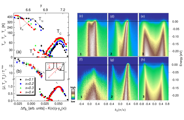
Figure 1: (a) The phase diagram of CLBLCO showing the Néel ($T_{N}$), glass ($T_{g}$) and superconducting ($T_{c}$) temperatures over the full doping range for the four families. $y_{N}$ indicates the oxygen level where $T_{N}$ start to drop. (b) The unified phase diagram of CLBLCO. The critical temperatures, and $J$ extracted from $T_{N}$, are divided by $T_{c}^{max}$ and plotted as a function of doping variation in the oxygen orbital $\Delta n_{p_{\sigma}}$. (c)-(e) Raw ARPES date measured on a CLBLCO $x=0.1$ crystal at $T=16$ K. The numbers on the figures correspond to cut trajectories illustrated in the inset of the phase diagram. (f)-(h) The same as (c)-(e) but for a sample with $x=0.4$ measured at $T=11$ K.

The ARPES experiments were performed on the SIS beam-line at the Swiss Light Source on CLBLCO single crystals. These unique crystals were grown using the traveling floating zone method. A detailed discussion about growth and characterization of these crystals is given in Crystal . For this experiment, samples with $x=0.1$ and $x=0.4$ were used. The samples were mounted on a copper holder with silver glue to improve electrical conductivity. The Fermi level and resolution were determined from the polycrystalline copper sample holder. The samples were cleaved in situ using a glued-on pin at $T=10-20$ K. Circularly polarized light with $h\nu=50$ eV was used. The spectra were acquired with a VG Scienta R4000 electron analyzer. Despite a base pressure of $5\times 10^{-}11$ torr, the samples’ surface life-time was only a few hours and a high intensity beam was required for quick measurements. As a consequence, the energy resolution in our experimental conditions was limited to $17-22$ meV.

In Fig. 1, we present ARPES data collected from CLBLCO for the two samples: $x=0.1$ is presented in panels c, d, and e, while $x=0.4$ is depicted in panels f, g, and h. The data was collected at $T=16$ K and $11$ K for the $x=0.1$ and $0.4$ respectively. All spectra are normalized by the measured detector efficiency. For each sample, intensities along three cuts are shown. The cuts are illustrated and numbered on the Fermi surface (FS) drawing in the inset of Fig. 1(b). Cuts numbered 1 and 2 are along $k_{x}$ ($\Gamma-M$ direction). These cuts allow better sensitivity to the gap size at the antinode. Cut number 3 is along the diagonal line of the BZ ($\Gamma-Y$). In this configuration, a measurement of velocity in the nodal direction is possible. The number on the bottom of each ARPES panel indicates the cut from which data are collected.

In Figs. 1(c) and 1(f), spectra near the anti-node are plotted. While $x=0.1$ shows high intensity spectra up to $E_{f}$ where no gap is visible, the $x=0.4$ sample shows a depletion of intensity close to $E_{f}$, indicating a gap in the spectra at the antinode. For the $x=0.1$, the gap, if one exists, is smaller than the experimental resolution. In Figs. 1(d) and 1(g), we plot the intensity closer to the node. For both the $x=0.1$ and $0.4$ sample, we clearly see the spectra crossing $E_{f}$ indicating a closed gap in the nodal region. Finally, in Figs. 1(e) and 1(h), both nodal cuts are seen, and again, the spectra cross $E_{f}$, indicating an absence of a gap along the Fermi arc for both samples. The last panels also show a clear dispersion from which the nodal velocity is extracted.

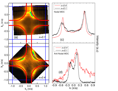
Figure 2: (a)-(b) Spectral weight map in $\mathbf{k}$-space at $E_{f}$ (FS) in CLBLCO $x=0.1$ and $x=0.4$ sample, respectively. The data were obtained at T=16 K for the $x=0.1$ sample and at T=11 K for the $x=0.4$ sample. Both samples were prepared with optimal doping and verified with a SQUID magnetometer. The red curve is the FS of CLBLCO obtained from tight binding fits to experimental data (see text). (c) MDCs at zero binding energy along a nodal cut, for the $x=0.1$ (black, Fig. 1(e)) and $x=0.4$ (red, Fig. 1(h)) samples. (d) MDCs at zero binding energy along the antinodal cut, for the $x=0.1$ (black, Fig. 1(d)) and $x=0.4$ (red, Fig. 1(g)) samples.

In Fig. 2, we show the FS in the first Brillouin zone (BZ), for the two CLBLCO samples: $x=0.1$ (Fig. 2(a)) and $0.4$ (Fig. 2(b)). The FS was obtained by integrating 10 meV around the chemical potential. The ARPES intensity is displayed in a false color scale as a function of $k_{x}$ and $k_{y}$. By comparing the shape of the FS, we can see that the $x=0.4$ sample exhibits a Fermi arc structure kanigel-arcs , which is typical for an antinodal gap. As for the $x=0.1$ sample, the arc is not present, and we observed strong intensity at the antinode, comparable to the intensity near the nodal region. Unlike previously reported FS measurements of YBCO k-ybco , there is no apparent chain-like structure in the CLBLCO FS, as expected. The red line is a fit to a tight binding (TB) model up to three nearest neighbours hopping. The fit parameters will be discussed below. The fit for both FSs gives the same size, as can be seen in Fig.2. In fact, the FS of a variety of samples was measured and found to be identical regardless of family ($x$) or bulk oxygen level ($y$).

A clearer comparison of the FS size and doping between families can be obtained by examining the node-to-node and antinodal distances. In Fig 2(c), we show momentum distribution curves (MDC) at zero binding energy ($E_{f}$) measured in a nodal cut (”cut 3”), for both samples. The MDC for $x=0.4$ is sharper than for $x=0.1$, but the peak-to-peak distance is equal for both MDCs. Similarly, Figure 2(d) depicts an MDC measured in the antinode (”cut 2”) at $E_{f}$. Here, the MDC of $x=0.1$ is clearer than that of $x=0.4$ because of an open gap, but again the peak separation for both samples is identical.

We suspect that the bulk doping independence of the FS is due to the sample being cleaved on a charged plane, inducing surface charge reconstruction. Such behavior was previously reported from measurements of YBCO k-ybco . From the measured nodal peak-to-peak distance as a function of doping in YBCO described in k-ybco , we can estimate the doping of our sample, which turns out to be $p=0.23\pm 0.02$. This result is consistent with calculations based on the FS volume. Thus, we can conclude that the surface doping level of both samples is equal within the experimental error, and that the surface doping is on the edge of the superconducting dome on the overdoped side.

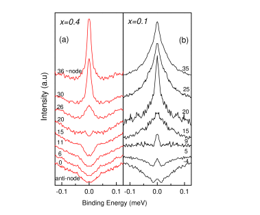
Figure 3: (a) Symmetrized EDCs for the $x=0.4$ sample at $k_{f}$ as a function of the Fermi surface angle $\phi$, from the node (top) to the anti-node (bottom). The cuts are measured along the $\Gamma-M$ direction. Each curve is offset for clarity. (b) the same as (a) but for the $x=0.1$ sample.

To investigate the momentum dependence of the gap, we measured the dispersion along $\Gamma-M$ cuts between “cut 1” and “cut 2” for the $x=0.1$ and $x=0.4$ samples at a cold finger temperature of $T=16$ K and $T=11$ K, respectively. In Fig. 3, we plot symmetrized EDC’s at $k_{f}$ as a function of FS angle $\phi$ (defined in the inset of Fig 1). For the $x=0.4$ sample (Fig. 3(a)), one can see a zero-energy intensity peak close to the node ($\phi=36$). In contrast, at an angle of $\phi=20$ and lower, we observe an opening of a gap, which grows up to $\Delta_{0}=40$ meV at the antinode ($\phi=0$). The angular dependence of the gap is shown in Fig.1 of the supplementary material. The gap value at the antinode is similar to optimally doped Bi2212 gap-doping-bssco ; mesot-bi2212gap and YBCO gap-ybco ; YBCO-gap-shen .

For the $x=0.1$ sample [Fig. 3(b)], the situation is different. Close to the node, we observe a strong peak at zero energy ($\phi=35$). As we move to the antinode, the intensity at zero energy is partly suppressed, but unlike the $x=0.4$ sample, there is no full depletion of spectral density at $E=0$. This indicates that a gap is not present in the $x=0.1$ sample, or that it is smaller than the experimental resolution ($20$ meV). A closed gap was measured with the same resolution for two more $x=0.1$ samples. Thus, we can safely say that $\Delta_{0}(x=0.4)>\Delta_{0}(x=0.1)$.

Last but not least, we compare the nodal velocity between families. This study was performed on six $x=0.1$ and seven $x=0.4$ crystals. The dispersion in the nodal direction, previously described in Fig 1(e,h), was measured for each sample in two branches with high statistics. After an orientation procedure, which is described in the supplementary material, the peak positions in the MDC of each measured dispersion was extracted and plotted as a function of binding energy. Exemplary dispersions of two samples are shown in Fig. 4. An axis breaker is used in order to show the two branches. The breaker emphasizes the differences between $k_{f}$ of the two samples, which in fact is very small. Two different linear regimes are observed. The first regime involves low energies close to $E_{f}$, between $-50<E<0$ meV. The second regime corresponds to high energies where $-150<E<-50$ meV. The transition between these regimes is known as the kink and involves the electrons dispersion re-normalized due to correlations Sato-Renormalization or coupling between electrons and low energy bosonic degrees of freedom LanzaraNature01 . The slope of the dispersion $\partial E/\partial k$ provides the velocity in the low ($v_{F}$) and high-energy (${v}_{HE}$) regimes. The results are similar to other overdoped materials ZhouNature03 .

We did not find differences with statistical significance in $v_{F}$ between samples with different $x$. This is in agreement with previous work ZhouNature03 . As for ${v}_{HE}$, the results are summarized in the inset of Fig. 4 as histograms. For the $x=0.1$ family, the average high-energy velocity is $\left\langle{V}_{HE}^{0.1}\right\rangle=1.53(04)$ eV$\mathring{A}$, while for the $x=0.4$ it is $\left\langle{V}_{HE}^{0.4}\right\rangle=1.73(04)$ eV$\mathring{A}$. Despite the velocity distribution overlap, the average velocities differ by 3.5$\sigma$, and hence are statistically different with 99.5% confidence. Using these velocities we can now calculate all the TB coefficients by $\partial E/\partial k=4at\sin(k_{f}^{node}a)$. The unit cell parameter $a=3.91$ Å is nearly family independent OferPRB08 . The coefficient are presented in the supplementary material and are in agreement with previously published values Bansil-TB NormanTBBSSCO .

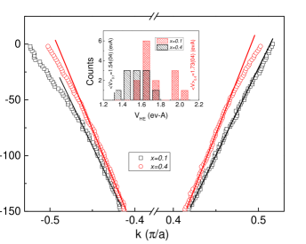
Figure 4: Main: The MDC peak position, extracted from the nodal dispersion measured along $\Gamma-Y$, as a function of $k$ for $x=0.1$ (black squares) and $x=0.4$ (red circles). Note the axis breaker. The solid lines are a linear fit to the data in the $-150<E<-50$ meV range from which the high energy velocities $V_{HE}$ are extracted. Inset: A histogram of high energy velocities obtained from a series of CLBLCO samples with $x=0.1$ (black, filled) and $x=0.4$ (red, crossed).

From the data presented, we can draw several conclusions. First, we discuss the ratio of velocities ${\left({\left\langle{{V_{HE}^{0.4}}}\right\rangle/}\left\langle{{V_{HE}^{0.1}}}\right\rangle\right)^{2}}\simeq 1.26\pm 0.08$. Despite the large error-bar, this ratio is very close to that expected from the ratio of the super-exchange $J$ between families. This ratio is given by $J(0.4)/J(0.1)=T_{c}^{max}(0.4)/T_{c}^{max}(0.1)\simeq 1.4$ (see Fig. 1). Therefore, the $J\propto t^{2}$ relation is obeyed, and $T_{c}^{max}$ depends on orbital overlaps even when the measurements are done in the doped phase.

However, ARPES measurements do not necessarily represent the bulk properties. For example, the buckling angle might change close to the surface. Nevertheless, if such a thing happens in CLBLCO, it might affect both families equally. The fact that the ratio of $J$ measured magnetically agrees with the ratio of $t^{2}$ measure by ARPES supports this notion.

Second, we discuss the gap. There are three possible scenarios that explain the difference in the gap size: I) A scenario where disorder leads to broadening of the band structure features in $x=0.1$ which hide the gap. However, high-resolution powder x-ray diffraction Xray and NMR experiments KerenNJP09 indicate that $x=0.1$ samples are more ordered than $x=0.4$ ones. II) A scenario where $\Delta$ exist only below $T_{c}$. It could be that in our experiment the surface of the $x=0.4$ sample is below $T_{c}$, but the $x=0.1$ surface, is not since its $T_{c}$ is lower. In this case only the $x=0.4$ sample will show a gap. The problem with this scenario is the observation of a Fermi arc in $x=0.4$, which does not exist below $T_{c}$ in any other cuprate. III) A scenario where both samples are above $T_{c}$, but there is an intrinsic difference in their gap size. The problem here is again that in other materials there is no gap above $T_{c}$ in extreme overdoped samples Chatterjee . Further experiments are needed to clarify this point.

In conclusion, we present the first ARPES data from CLBLCO. We find that the surface doping is independent of the bulk doping or the Ca to Ba ratio. We also demonstrate that the gap can be measured in this system. The hopping parameter $t$ is larger for $x=0.4$ than for $x=0.1$ in the over-doped sides. This suggests that $T_{c}^{max}$ is correlated with electron-orbital overlaps on neighboring sites.

This research was supported by the Israeli Science Foundation (ISF) and the joint German-Israeli DIP Project.

I Supplementary Material for Linking Dynamic and Thermodynamic Properties of Cuprates; an ARPES study of (CaLa)(BaLa)₂Cu₃O_y.

I.1 Gap Angular Dependence

In Figure 5 we plot the gap size as a function of Fermi surface angle for the $x=0.4$ sample. The value of gap, extracted from the symmetrized EDC’s shown in the article, is half of the peak-to-peak distance or the change in slope of the EDC.

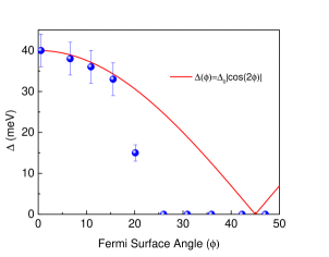
Figure 5: Gap size as a function of Fermi surface angle $\phi$ for the $x=0.4$ sample. The red line is the d-wave gap function, $\Delta(\phi)=\Delta_{0}|\cos(2\phi)|$, with $\Delta_{0}=40$ meV.

I.2 Nodal Cut Measurement

Because of the importance of proper orientation for the determination of the nodal velocity, we developed an alignment protocol. First, we map the complete FS of each sample in the first BZ. We define three angles, which can be manipulated, as shown in the inset of Fig. 6(a). $\theta=0$ , $\varphi=45$, and $\psi$ $=0$ define a nodal cut. The red strait line represents the analyzer opening. Second, the angle $\theta$ is adjusted to give a symmetric spectrum. Third, we performed measurements with an intentional shifts $\Delta\psi$ and $\Delta\varphi$ angle to ensure truly perfect alignment. From each measurement we extracted the $k-$space distance $\Delta k(\Delta\psi,\Delta\varphi)$ between the two Fermi points. Figure 6(a) presents $\Delta k(\Delta\psi,0)$ for $\psi$ variations in steps of 0.5 a degrees. Figure  6(b) depicts $\Delta k(0,\Delta\varphi)$ for $\varphi$ rotations again in steps of 0.5 degrees. Due to the geometry of the FS the nodal distance should be shortest when the alignment is perfect. Indeed, in both cases, the shortest distance was measured when $\Delta\psi=\Delta\varphi=0$. This procedure was repeated for each and every measured sample.

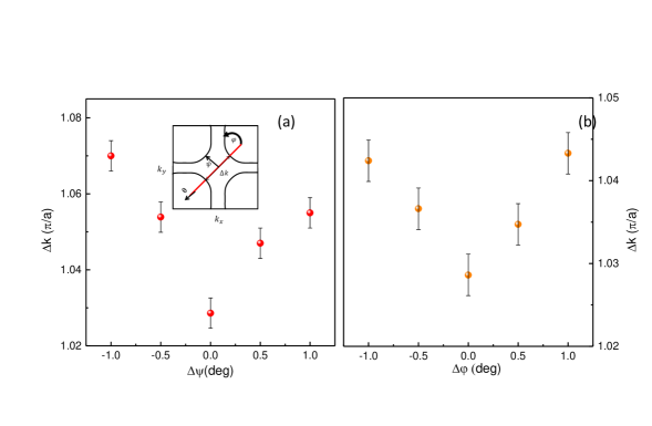
Figure 6: (a) The nodal distance $\Delta k$ as a function of the change in angle $\psi$, and (b) as a function of the change in angle $\varphi$. The inset shows an illustration of a nodal cut upon a FS, with the definition and action of $\theta,\varphi$ and $\psi$ angles used in the experiment

I.3 Tight Binding Parameters

The tight binding parameters for CLBLCO extracted from the Fermi surface and nodal velocity are given in the table.

i	$t_{i}^{x=0.1}$	$t_{i}^{x=0.4}$	$\eta_{i}(\mathbf{k})$
0	0.134	0.152	1
1	0.110	0.125	$-2\left[{\cos\left({{k_{x}}a}\right)+\cos\left({{k_{y}}a}\right)}\right]$
2	-0.032	-0.036	$-4\left[{\cos\left({{k_{x}}a}\right)\cos\left({{k_{y}}a}\right)}\right]$
3	0.016	0.018	$-2\left[{\cos\left({2{k_{x}}a}\right)+\cos\left({2{k_{y}}a}\right)}\right]$

Table 1: Tight-binding coefficients and basis functions used to fit the experimental data. The second column lists the coefficient of each term in eV for the $x=0.1$ and $x=0.4$ samples, following the convention: $\varepsilon\left(\mathbf{k}\right)=\sum{{t_{i}}{\eta_{i}}\left(\mathbf{k}\right)}$

References

- (1) G. Drachuck et al., Journal of Superconductivity and Novel Magnetism 25, 2331-2335, (2012), 10.1007/s10948-012-1669-z.
- (2) Bernhard Edegger, V. N. Muthukumar, Claudius Gros, and P.W. Anderson, Phys. Rev. Lett 96, 207002 (2006), 10.1103/PhysRevLett.96.207002; E. Pavarini, I. Dasgupta, T. Saha-Dasgupta, O. Jepsen, and O. K. Andersen, Phys. Rev. Lett. 87, 047003 (2001), 10.1103/PhysRevLett.87.047003.
- (3) A. Knizhnik et al., Physica C 321, 199, (1999), 10.1016/S0921-4534(99)00363-9.
- (4) E. Amit and A. Keren, Phys. Rev. B 82, 172509 (2010), 10.1103/PhysRevB.82.172509.
- (5) R. Ofer, A. Keren, O. Chmaissem, and A. Amato, Phys Rev. B 78, 140508(R) (2008), 10.1103/PhysRevB.78.140508.
- (6) R. Ofer et al., Phys. Rev. B 74, 220508(R) (2006), 10.1103/PhysRevB.74.220508.
- (7) Dirk Wulferding, Raman vs SR in CLBLCO, In prepration.
- (8) Henk Eskes and Robert Eder, Phys. Rev. B 54, R14226 (1996), 10.1103/PhysRevB.54.R14226.
- (9) Le Tacon et al., Nature Physics 7, 725 (2011); M. P. M. Dean et al., Nature Materials 12, 1019 (2013).
- (10) Kanigel A. et al., Nature Physics 2, 447 - 451 (2006), doi:10.1038/nphys334.
- (11) M. A. Hossain et al., Nature Physics 4, 527 (2008); Fournier, D. et al., Nature Physics 6, 905-911 (2010), doi:10.1038/nphys1763.
- (12) Chatterjee, U. et al. Nature Physics 6, 99 - 103 (2010), doi:10.1038/nphys1763.
- (13) J. Mesot et al., Phys. Rev. Lett. 83, 840-843 (1999), 10.1103/PhysRevLett.83.840.
- (14) Lu D.H. et al., Phys. Rev. Lett. 86 4370-4373, (2001), 10.1103/PhysRevLett.86.4370.
- (15) Sutherland M. et al., Physica C 408-410, 672-673, (2004), doi/10.1016/j.physc.2004.03.104.
- (16) Sato T.et al. Phys. Rev. Lett. 91, 157003 (2003), 10.1103/PhysRevLett.91.157003.
- (17) Lanzara, A. et al., Narure 412, 510-514, (2001), doi:10.1038/35087518.
- (18) X. J. Zhou, T. Yoshida, A. Lanzara, P. V. Bogdanov, S. A. Kellar, K. M. Shen, W. L. Yang, F. Ronning, T. Sasagawa, T. Kakeshita, T. Noda, H. Eisaki, S. Uchida, C. T. Lin, F. Zhou, J. W. Xiong, W. X. Ti, Z. X. Zhao, A. Fujimori, Z. Hussain and Z.-X. Shen, Nature 423, 398 (2003), doi:10.1038/423398a
- (19) Markiewicz, R. S et al., Phys. Rev. B 72 054519 (2005), 10.1103/PhysRevB.72.054519.
- (20) Norman, M. R. et al., Phys. Rev. B 52, 615-622 (1995), 10.1103/PhysRevB.52.615.
- (21) S. Agrestini, S. Sanna, K. Zheng, R. De Renzi, E. Pusceddu, G. Concas, N. L. Saini, A. Bianconi, cond-mat 1310.0659.
- (22) A. Keren, New J. Phys. 11 065006 (2009).
- (23) U. Chatterjee, J. Zhao, D. Ai, S. Rosenkranz, A. Kaminski, H. Raffy, Z. Z. Li, K. Kadowaki, M. Randeria, M. R. Norman, and J. C. Campuzano, PNAS 108, 9346 (2011).