Open Boundary Condition, Wilson Flow and the Scalar Glueball Mass

Abstract

A major problem with periodic boundary condition on the gauge fields used in current lattice gauge theory simulations is the trapping of topological charge in a particular sector as the continuum limit is approached. To overcome this problem open boundary condition in the temporal direction has been proposed recently. One may ask whether open boundary condition can reproduce the observables calculated with periodic boundary condition. In this work we find that the extracted lowest glueball mass using open and periodic boundary conditions at the same lattice volume and lattice spacing agree for the range of lattice scales explored in the range $3~{}{\rm GeV}\leq\frac{1}{a}\leq 5$ GeV. The problem of trapping is overcome to a large extent with open boundary and we are able to extract the glueball mass at even larger lattice scale $\approx$ 5.7 GeV. To smoothen the gauge fields we have used recently proposed Wilson flow which, compared to HYP smearing, exhibits better systematics in the extraction of glueball mass. The extracted glueball mass shows remarkable insensitivity to the lattice spacings in the range explored in this work, $3~{}{\rm GeV}\leq\frac{1}{a}\leq 5.7~{}{\rm GeV}$.

1 Motivation

Even though lattice QCD continues to make remarkable progress in confronting experimental data, certain problems have persisted. For example, the spanning of the gauge configurations over different topological sectors become progressively difficult as the continuum limit is approached. This is partly intimately related to the use of periodic boundary condition on the gauge field in the temporal direction of the lattice. As a consequence, in the continuum limit, different topological sectors are disconnected from each other. Thus at smaller and smaller lattice spacings the generated gauge configurations tend to get trapped in a particular topological sector for a very long computer simulation time thus resulting in very large autocorrelations. This may sometime even invalidate the results of the simulation. Open boundary condition on the gauge field in the temporal direction has been recently proposed to overcome this problem open0 ; open1 ; open2 . Usage of open boundary conditions has been found to be advantageous in a weak coupling study of SU(2) lattice gauge theory grady .

The spanning of different topological sectors can be studied through topological susceptibility ($\chi$) which is related to the $\eta^{\prime}$ mass by the Witten-Veneziano formula witten ; veneziano ; seiler in pure Yang-Mills lattice theory. For example, some high precision calculations of $\chi$ on periodic lattices are provided in Refs. del ; durr ; lspb . In Ref. opentopo , we have addressed the question whether open boundary condition in the temporal direction can yield the expected value of $\chi$. We have shown that with the open boundary it is possible to get the expected value of $\chi$ and the result agrees with our own numerical simulation employing periodic boundary condition.

We continue our exploration of open boundary condition in this work, in the context of extraction of lowest glueball mass from the temporal decay of correlators. Extraction of glueball masses compared to hadron masses is much more difficult due to the presence of large vacuum fluctuations present in the correlators of gluonic observables. Moreover the computation of low lying glueball masses which are much higher than the masses of hadronic ground states, in principle requires relatively small lattice spacings. To overcome these problems, anisotropic lattices together with improved actions and operators have been employed mp1 ; mp2 ; chen successfully to obtain accurate glueball masses. On the other hand, the calculation of glueball masses with isotropic lattice has a long history (see for example, the reviews, Refs. teprev ; balirev ). These calculations which employ periodic boundary condition in the temporal direction have been pushed to lattice scale of $a^{-1}=3.73(6)$ GeV baliplb ; vaccarino . One would like to continue these calculations to even higher lattice scale which however eventually will face the problem of efficient spanning of the space of gauge configurations. Such trapping has been already demonstrated opentopo . It is interesting to investigate whether the open boundary condition can reproduce the glueball masses extracted with periodic boundary condition at reasonably small lattice spacings achieved so far and whether the former can be extended to even smaller lattice spacings. Our main objective in this paper is to address these issues.

An important ingredient in the extraction of masses is the smearing of gauge field which is necessary both to suppress unwanted fluctuations due to lattice artifacts and to increase the ground state overlap parisi . In the past various techniques have been proposed towards smearing the gauge fields ape ; hyp ; morningstar . Recently proposed Wilson flow wf1 ; wf2 ; wf3 puts the technique of smearing on a solid mathematical footing. The same idea is referred to in the mathematical literature by the name of gradient flow atbott ; gtp ; mani . Another motivation of the present work is the study of the effectiveness of Wilson flow in the extraction of masses.

2 Simulation details

Lattice	Volume	$\beta$	$N_{\rm cnfg}$	$N_{0}$	$\tau$	$a[{\rm fm}]$	$t_{0}/a^{2}$
$O_{1}$	$24^{3}\times 48$	6.21	3970	12	3	0.0667(5)	6.207(15)
$O_{2}$	$32^{3}\times 64$	6.42	3028	20	4	0.0500(4)	11.228(31)
$O_{3}$	$48^{3}\times 96$	6.59	2333	26	5	0.0402(3)	17.630(53)
$O_{4}$	$64^{3}\times 128$	6.71	181	64	10	0.0345(4)	24.279(227)
$P_{1}$	$24^{3}\times 48$	6.21	3500	12	3	0.0667(5)	6.197(15)
$P_{2}$	$32^{3}\times 64$	6.42	1958	20	4	0.0500(4)	11.270(38)
$P_{3}$	$48^{3}\times 96$	6.59	295	26	5	0.0402(3)	18.048(152)

Table 1: Simulation parameters for the HMC algorithm. $N_{0}$ is the number of integration steps, $\tau$ is the trajectory length and $t_{0}/a^{2}$ is the dimensionless reference Wilson flow time. $O$ and $P$ refer to ensembles with open and periodic boundary condition in the temporal direction.

Using the openQCD program openqcd , SU(3) gauge configurations are generated with open boundary condition (denoted by $O$) at different lattice volumes and gauge couplings. For comparison purposes, we have also generated gauge configurations (denoted by $P$) for several of the same lattice parameters by implementing periodic boundary condition in temporal direction in the openQCD package. In table 1, we summarize details of the simulation parameters.

To extract the scalar glueball mass, in this initial study we use the correlator of $\overline{E}$ which is the average of the action density over spatial volume at a particular time slice given in Ref. open1 . Since the action is a sum over the plaquettes, this is similar to the use of plaquette-plaquette correlators which have been used in the literature berg ; billorie . As in the latter case, there is room for operator improvement. One may use simple four link plaquette (unimproved) or one may use the clover definition of the field strength in the action (improved).

Correlator is measured over $N_{\rm cnfg}$ number of configurations. The separation by $32$ is made between two successive measurements. Thus the total length of simulation time is $N_{\rm cnfg}\times 32$. Using the results from Refs. gsw ; necco , we have determined the lattice spacings which are quoted in table 1. We have employed Wilson flow wf1 ; wf2 ; wf3 to smooth the gauge configurations. The implicit equation

$$\big{\{}t^{2}\langle\overline{E}(T/2)\rangle\big{\}}_{t=t_{0}}=0.3$$ (1)

with $t$ and $T$ being respectively the Wilson flow time and the temporal extent of the lattice, defines a reference flow time $t_{0}$ which provides a reference scale to extract physical quantities from lattice calculations. No significant difference has been found in our results using the $w_{0}$ scale proposed in Ref. wscale as an alternative to the $t_{0}$ scale.

3 Numerical Results

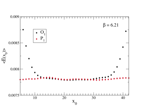
Figure 1: Plot of $\langle\overline{E}(x_{0})\rangle$ versus $x_{0}$ at flow time $t=t_{0}$ at $\beta=6.21$ and lattice volume $24^{3}\times 48$ for ensemble $O_{1}$ (filled circle) and ensemble $P_{1}$ (filled square).

Since we extract the scalar glueball mass from the temporal decay of the correlator of $\overline{E}(x_{0})$ where $x_{0}$ denotes the particular temporal slice, we first look at the effect of open boundary on the $\langle\overline{E}(x_{0})\rangle$. In figure 1 we plot $\langle\overline{E}(x_{0})\rangle$ versus $x_{0}$ at flow time $t=t_{0}$ at $\beta=6.21$ and lattice volume $24^{3}\times 48$ for ensemble $O_{1}$. Breaking of translational invariance due to open boundary condition in the temporal direction is clearly visible in the plot. To calculate the correlator we need to pick the sink and source points from the region free from boundary artifacts, which can be identified from such plot. To facilitate the identification better, we also plot $\langle\overline{E}(x_{0})\rangle$ for periodic boundary condition in the temporal direction for the same lattice volume and lattice spacing (ensemble $P_{1}$). Preservation of translation invariance is evident in this case. Clearly, for open boundary condition, source and sink points need to be chosen from the region where $\langle\overline{E}(x_{0})\rangle$ is almost flat. We note that for both open and periodic cases the central region $\langle\overline{E}(x_{0})\rangle$ is not perfectly flat but exhibits an oscillatory behaviour on a fine scale.

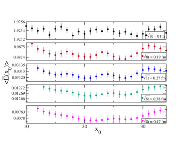
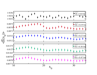
Figure 2: Plot of $\langle\overline{E}(x_{0})\rangle$ versus $x_{0}$ at various flow times $t$ at $\beta=6.21$ and lattice volume $24^{3}\times 48$ for ensemble $O_{1}$ (left) and for ensemble $P_{1}$ (right).

To understand the oscillatory behaviour, in figure 2 we plot $\langle\overline{E}(x_{0})\rangle$ versus $x_{0}$ at various flow times $t$ at $\beta=6.21$ and lattice volume $24^{3}\times 48$ for ensemble $O_{1}$ (left) and for ensemble $P_{1}$ (right). At small Wilson flow time, the fluctuations of $\langle\overline{E}(x_{0})\rangle$ are very large as seen from the top panel of the plots. To reduce the fluctuation we have to increase Wilson flow time. The comparison of different panels clearly demonstrates the reduction of fluctuations with increasing flow time (note that the scale on y axis becomes finer and finer as flow time increases). However, with increasing flow time the data become more correlated and longer wavelengths appear open2 . The plots show that this smoothening behaviour is the same for both the open and periodic boundary conditions.

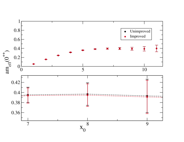
Figure 3: Plot of glueball effective mass $am_{eff}~{}(0^{++})$ versus the temporal difference $x_{0}$ at Wilson flow times $\sqrt{8t}=0.28~{}{\rm fm}$, $\beta=6.42$ and lattice volume $32^{3}\times 64$ for ensemble $P_{2}$ for improved and unimproved choices of operators. The lower panel shows the detail of the plateau region of the upper panel.

Next we discuss the extraction of glueball mass. As already discussed in section 2, one may use the unimproved (naive plaquette) or improved (clover) version of the operator $\overline{E}(x_{0})$. In general we expect improved operator to be preferable over unimproved one. However, for the extraction of masses Wilson flow is essential and this may diminish the difference between the results using them. In this work we have used Wilson flow in all the four directions as originally conceived. Due to the smearing in the temporal direction we should expect to get glueball mass for separation between source and sink which are larger than twice the smearing radius ($\approx 2\times\sqrt{8t}$). However a successful extraction of glueball mass in this case requires reasonably small statistical error at such large temporal separation. In figure 3 we plot glueball effective mass $am_{eff}~{}(0^{++})$ versus the temporal difference $x_{0}$ ($x_{0}=x_{0}^{{\rm source}}-x_{0}^{{\rm sink}}$) at Wilson flow time $\sqrt{8t}=0.28~{}{\rm fm}$, $\beta=6.42$ and lattice volume $32^{3}\times 64$ for ensemble $P_{2}$ for improved and unimproved choices of operators (from here onwards, we denote the temporal difference by $x_{0}$). As expected the plateau appears for relatively larger temporal separation and presumably thanks to Wilson flow the statistical error is reasonably small. We have verified that the results are very similar at all other Wilson flow times under consideration. Even though we find that there is no noticeable difference between them, we employed the improved operator for the rest of the calculations in this paper.

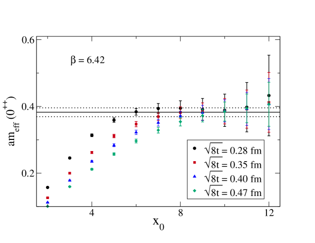
Figure 4: Plot of lowest glueball effective mass $am_{eff}~{}(0^{++})$ versus $x_{0}$ at four different Wilson flow times $t$, $\beta=6.42$ and lattice volume $32^{3}\times 64$ for ensemble $P_{2}$. Also shown is the fit to the plateau region of the data for $\sqrt{8t}=0.35$ fm.

We extract the effective mass for the glueball ($0^{++}$) state from the temporal decay of the correlator $\langle\overline{E}(x_{0}^{{\rm sink}})\overline{E}(x_{0}^{{\rm source}})\rangle$ where $x_{0}^{{\rm sink}}$ and $x_{0}^{{\rm source}}$ are the sink and source points in the temporal direction. To improve the statistics we have averaged over the source points when we employ periodic boundary condition on the temporal direction. Further to reduce fluctuations we have performed the Wilson flow up to flow time $t=t_{0}$. In figure 4 we plot the lowest glueball effective mass $am_{eff}~{}(0^{++})$ versus $x_{0}$ at four Wilson flow times $t$, $\beta=6.42$ and lattice volume $32^{3}\times 64$ for ensemble $P_{2}$. We find that the effective mass is sensitive to Wilson flow time for initial temporal differences $x_{0}$ but becomes independent of different Wilson flow times in the plateau region within statistical error. Note that as expected, the plateau region moves to the right as Wilson flow time increases. Also shown in the figure is the fit to the plateau region of the data for $\sqrt{8t}=0.35$ fm. The fit nevertheless passes through the plateau regions of data sets corresponding to other Wilson flow times.

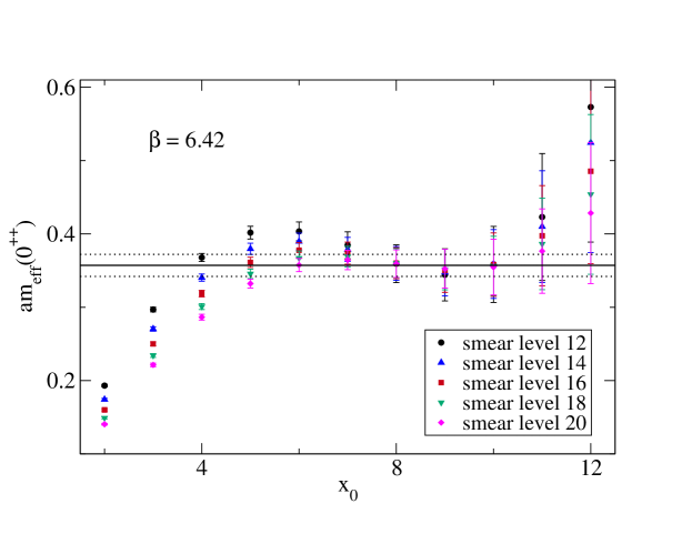
Figure 5: Plot of lowest glueball effective mass $am_{eff}~{}(0^{++})$ versus $x_{0}$ at five HYP smearing levels at $\beta=6.42$ and lattice volume $32^{3}\times 64$ for ensemble $P_{2}$. Also shown is the fit to the plateau region of the data for smear level 18.

For comparison with traditional methods to smoothen the gauge field configurations, in figure 5 we plot the lowest glueball effective mass $am_{eff}~{}(0^{++})$ versus $x_{0}$ at five smearing levels for four dimensional HYP smearing hyp at $\beta=6.42$ and lattice volume $32^{3}\times 64$ for ensemble $P_{2}$. We find that the effective mass for different smear levels converge in a very narrow window where we can identify the plateau region and extract the mass. This behaviour is to be contrasted with that in the case of Wilson flow discussed in the previous paragraph. Also shown in the figure is the fit to the plateau region of the data for smear level 18. In physical units the fitted mass is found to be 1409 (59) MeV which has a marginal overlap with the same [1510 (52) Mev] obtained with Wilson flow. We have observed from our studies with all the $\beta$ values that the results obtained with HYP smearing are systematically lower than those obtained with Wilson flow. We note that the latter value is closer to the range of glueball mass quoted by other collaborations. The works presented in the rest of paper employ Wilson flow to smooth the gauge fields.

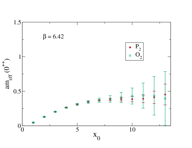
Figure 6: Comparison of lowest glueball mass $am_{eff}~{}(0^{++})$ versus $x_{0}$ at Wilson flow time ($\sqrt{8t}=0.35~{}{\rm fm}$), $\beta=6.42$ and lattice volume $32^{3}\times 64$ for ensembles $O_{2}$ and $P_{2}$.

With open boundary condition the translational invariance in the temporal direction is broken and hence we can not average over all the source points to improve statistical accuracy as we have done in the case of periodic boundary condition. Nevertheless, we can average over few source points chosen far away from the boundary. In figure 6 we plot the lowest glueball effective mass $am_{eff}~{}(0^{++})$ versus $x_{0}$ at Wilson flow time ($\sqrt{8t}=0.35~{}{\rm fm}$), $\beta=6.42$ and lattice volume $32^{3}\times 64$ for both open and periodic boundary conditions (ensembles $O_{2}$ and $P_{2}$). We find that effective mass agree for the two choices of the boundary conditions but as expected statistical error is larger for open boundary data.

Lattice	fit range	$am~{}(0^{++})$
$O_{1}$	7-9	0.569(69)
$P_{1}$	7-9	0.520(21)
$O_{2}$	9-12	0.419(57)
$P_{2}$	8-11	0.383(13)
$O_{3}$	10-12	0.327(39)
$P_{3}$	10-12	0.313(28)
$O_{4}$	7-10	0.274(48)

Table 2: Lattice glueball $0^{++}$ mass.

In table 2 we have shown the fit range used to extract and the extracted lattice glueball mass for the ensembles studied in this paper. A constant is fitted to extract the mass.

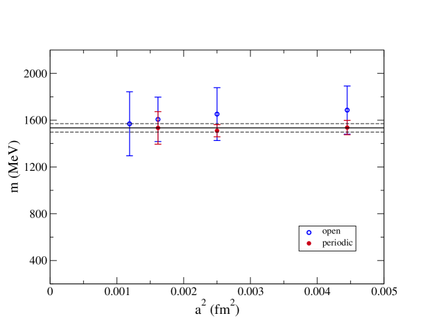
Figure 7: Plot of the lowest glueball mass $m~{}(0^{++})$ in MeV versus $a^{2}$ for both open and periodic boundary condition for different lattice spacings and lattice volumes. Also shown is the fit to the combined data.

To extract the continuum value of $0^{++}$ glueball mass, in figure 7 we plot $m~{}(0^{++})$ in MeV versus $a^{2}$ for both open and periodic boundary condition for different lattice spacings and lattice volumes. For the range of reasonably small lattice spacings explored in this work, remarkably, the data does not show any deviation from scaling within the statistical error. Hence we fit a constant to the combined data as shown in the figure and extract the continuum value of $0^{++}$ mass, 1534(36) MeV. We note that this value compares favorably with the range of glueball mass quoted in the literature.

4 Conclusions

In lattice Yang-Mills theory, we have shown that the open boundary condition on the gauge fields in the temporal direction of the lattice can reproduce the lowest scalar glueball mass extracted with periodic boundary condition at reasonably large lattice scales investigated in the range $3~{}{\rm GeV}\leq\frac{1}{a}\leq 5$ GeV. With open boundary condition we are able to overcome, to a large extent, the problem of trapping and performed simulation and extract the glueball mass at even larger lattice scale $\approx$ 5.7 GeV. Compared to HYP smearing, recently proposed Wilson flow exhibits better systematics as far as the extraction of glueball mass is concerned. The extracted glueball mass shows remarkable insensitivity to the lattice spacings in the range explored in this work $3~{}{\rm GeV}\leq\frac{1}{a}\leq 5.7~{}{\rm GeV}$.

Conventionally, due to various theoretical reasons, in the calculation of masses from correlators, smearing of gauge field is carried out only in spatial directions. In this work, however, Wilson flow is carried out in all the four directions and our results show that one can indeed extract mass with relatively small statistical error at relatively large temporal separations. A critical evaluation of the strengths and weaknesses of the four-dimensional versus three-dimensional smoothening of the gauge field in the calculation of masses is beyond the scope of the present work.

Acknowledgements Cray XT5 and Cray XE6 systems supported by the 11th-12th Five Year Plan Projects of the Theory Division, SINP under the Department of Atomic Energy, Govt. of India, are used to carry out all the numerical calculations reported in this work. For the prompt maintenance of the systems and the help in data management, we thank Richard Chang. We also thank Stephan Dürr and Martin Lüscher for helpful comments. This work was in part based on the publicly available lattice gauge theory code openQCD openqcd .

References

- (1) M. Lüscher, PoS LATTICE 2010, 015 (2010) [arXiv:1009.5877 [hep-lat]].
- (2) M. Lüscher and S. Schaefer, JHEP 1107, 036 (2011) [arXiv:1105.4749 [hep-lat]].
- (3) M. Lüscher and S. Schaefer, Comput. Phys. Commun. 184, 519 (2013) [arXiv:1206.2809 [hep-lat]].
- (4) M. Grady, arXiv:1104.3331 [hep-lat].
- (5) E. Witten, Nucl. Phys. B 156, 269 (1979).
- (6) G. Veneziano, Nucl. Phys. B 159, 213 (1979).
- (7) E. Seiler, Phys. Lett. B 525, 355 (2002) [hep-th/0111125].
- (8) L. Del Debbio, L. Giusti and C. Pica, Phys. Rev. Lett. 94, 032003 (2005) [hep-th/0407052].
- (9) S. Dürr, Z. Fodor, C. Hoelbling and T. Kurth, JHEP 0704, 055 (2007) [hep-lat/0612021].
- (10) M. Lüscher and F. Palombi, JHEP 1009, 110 (2010) [arXiv:1008.0732 [hep-lat]].
- (11) A. Chowdhury, A. Harindranath, J. Maiti and P. Majumdar, JHEP 02, 045 (2014) [arXiv:1311.6599 [hep-lat]].
- (12) C. J. Morningstar and M. J. Peardon, Phys. Rev. D 56, 4043 (1997) [hep-lat/9704011].
- (13) C. J. Morningstar and M. J. Peardon, Phys. Rev. D 60, 034509 (1999) [hep-lat/9901004].
- (14) Y. Chen, A. Alexandru, S. J. Dong, T. Draper, I. Horvath, F. X. Lee, K. F. Liu and N. Mathur et al., Phys. Rev. D 73, 014516 (2006) [hep-lat/0510074].
- (15) M. J. Teper, Glueball masses and other physical properties of SU(N) gauge theories in D = (3+1): A Review of lattice results for theorists, hep-th/9812187.
- (16) G. S. Bali, Glueballs’: Results and perspectives from the lattice, hep-ph/0110254.
- (17) G. S. Bali et al. [UKQCD Collaboration], Phys. Lett. B 309, 378 (1993) [hep-lat/9304012].
- (18) A. Vaccarino and D. Weingarten, Phys. Rev. D 60, 114501 (1999) [hep-lat/9910007].
- (19) G. Parisi, Prolegomena to any future computer evaluation of the QCD mass spectrum, in Progress in gauge field theory : proceedings, G. ’t Hooft, A. Jaffe, H. Lehmann, P.K. Mitter, I. M. Singer, R. Stora. (eds.), (Plenum Press, 1984).
- (20) M. Albanese, F. Constantini, G. Fiorentini, F. Flore, M. P. Lombardo, R. Tripiccione, P. Bacilieri, L. Fonti, P. Giacomelli, E. Remiddi, M. Bernaschi, N. Cabibbo, E. Marinari, G. Parisi, G. Salina, S. Cabasino, F. Marzano, P. Paolucci, S. Petrarca, F. Rapuano and P. Marchesini, Phys. Lett. B192, 163 (1987).
- (21) A. Hasenfratz, F. Knechtli, Phys. Rev. D 64 (2001) 034504, hep-lat/0103029
- (22) C. Morningstar and M. J. Peardon, Phys. Rev. D 69, 054501 (2004) [hep-lat/0311018].
- (23) M. Lüscher, Commun. Math. Phys. 293, 899 (2010) [arXiv:0907.5491 [hep-lat]].
- (24) M. Lüscher, JHEP 1008, 071 (2010) [arXiv:1006.4518 [hep-lat]].
- (25) M. Lüscher and P. Weisz, JHEP 1102, 051 (2011) [arXiv:1101.0963 [hep-th]].
- (26) M. F. Atiyah and R. Bott, The Yang-Mills Equations over Riemann Surfaces, Philosophical Transactions of the Royal Society of London. Series A, Mathematical and Physical Sciences, Vol. 308, No. 1505 (Mar. 17, 1983), pp. 523-615
- (27) M. Nakahara, Geometry, Topology and Physics, Second edition, Taylor and Francis (2003).
- (28) S. K. Donaldson and P. B. Kronheimer, The Geometry of Four-Manifolds, Oxford University Press, USA (1997).
- (29) http://luscher.web.cern.ch/luscher/openQCD/
- (30) B. Berg, Phys. Lett. B 97, 401 (1980).
- (31) B. Berg and A. Billoire, Nucl. Phys. B 226, 405 (1983).
- (32) M. Guagnelli et al. [ALPHA Collaboration], Nucl. Phys. B 535, 389 (1998) [hep-lat/9806005].
- (33) S. Necco and R. Sommer, Nucl. Phys. B 622, 328 (2002) [hep-lat/0108008].
- (34) S. Borsanyi, S. Dürr, Z. Fodor, C. Hoelbling, S. D. Katz, S. Krieg, T. Kurth and L. Lellouch et al., JHEP 1209, 010 (2012) [arXiv:1203.4469 [hep-lat]].