Static consensus in passifiable linear networks

Abstract

Sufficient conditions of consensus (synchronization) in networks described by digraphs and consisting of identical determenistic SIMO systems are derived. Identical and nonidentical control gains (positive arc weights) are considered. Connection between admissible digraphs and nonsmooth hypersurfaces (sufficient gain boundary) is established. Necessary and sufficient conditions for static consensus by output feedback in networks consisting of certain class of double integrators are rediscovered. Scalability for circle digraph in terms of gain magnitudes is studied. Examples and results of numerical simulations are presented.

1 Introduction

Control of multi-agent systems has attracted significant interest in last decade since it has a great technical importance [6, 21, 22, 23] and relates to biological systems [24].

In consensus problems agents communicate via decentralized controllers using relative measurements with a final goal to achieve common behaviour (synchronization) which can evolve in time. Many approaches have been developed for a different problem settings.

Laplace matrix, its spectrum, and eigenspace plays crucial role in description and analysis of consensus problems. It has broad applications, e.g. [13]. Not all possible digraph topologies can provide consensus over dynamical networks. Admissible digraph topologies and connection with algebraic properties of Laplace matrix have been found in [1]. Analysis of tree strucure and Laplace matrices spectrum of digraphs are also studied by these authors. Work [8] contains examples of out-forests as well as useful graph theoretical concepts and can be recommended as an entry reading to the research of these authors on algebraic digraph theory and consensus problems.

Concept of synchronization region in complex plane for a networks consisting of linear dynamical systems is introduced in [19]. In [27] this concept is used for analysis of synchronization with leader. Problem is solved using Linear Quadratic Regulator approach in cases when full state is available for measurement and when its not. In last case observers are constructed.

Analysis of consensus with scalar coupling strenghts [19, 27] is fruitful in a sense that conditions on gains (which depend on connection topology and single agent properties) give more insight to problem. A lot of works on topic consider dynamic couplings, however, for certain type of connections it might happen that tunable parameters will exceed upper bound on possible control gains, i.e. won’t meet physical limitations. So, necessary and sufficient conditions on consensus achievement for different connection types in terms of coupling strenghts are needed.

Celebrated Kalman-Yakubovich-Popov Lemma (Positive Real Lemma) establishes important connection between passivity (positive-realness) of transfer function $\chi(s)$ and matrix relations on its minimal state-space realization $(A,B,C),$ see [5, 17]. Positive Real Lemma is a basis for Passification Method [11, 12] (“Feedback Kalman-Yakubovich Lemma”) which answers question when a linear system can be be made passive, i.e. strictly positive-real (SPR) by static output feedback. Powerful idea of rendering system into passive by feedback have been also studied for nonlinear systems, e.g. [7, 17, 18].

In consensus-type problems considering SPR agents with stable (Hurwitz) matrix $A$ leads to a synchronous behaviour when all states going to zero. Latter is undesirable in essence, since such behaviour can be reached by local control without communication. So, instead of SPR systems it is possible to consider passifiable systems, with an opportunity that a study is extendable to nonlinear systems. Also, Passification Method allows to avoid constructing observers for reaching full-state consensus by output feedback. Observers implementation increase dimension of overall phase space and Complexity of a dynamic network.

In this paper Passification Method are used to synthesize a decentralized control law and to derive sufficient conditions of full state synchronization by relative output feedbacks in a networks described by digraphs with Linear Time Invariant dynamical nodes in continuous time. Assumptions made on network topology are minimal. Synchronous behaviour is described, including case of nonidentical gains. It is determined that boundary of sufficient gain region geometrically is a hypersurface in corresponding gain space. For certain three node network this geometrical observation connects algebraic properties of Laplace matrix with constructed hypersurface. Namely, Jordan block appears in a direction of a cusp (nonsmooth) extremal point of the hypersurface.

Necessary and sufficient conditions for static consensus by output feedback in networks consisting of certain class of double integrators have been rediscovered. Conditions are given in terms of Laplace matrix spectrum.

Scalability in a circle digraphs in terms of gain (coupling strength) is studied. It is shown that common gain in large cycle digraphs consisting of double integrators should grow not slower than quadratically in number of agents.

Results of numerical simulations in 3 and 20 node double-integrator networks are presented.

2 Theoretical study

2.1 Preliminaries and notations

Notations, some terms of graph theory and Passification Lemma are listed in this section.

2.1.1 Notations

Notation $\|.\|_{2}$ stands for Euclidian norm. For two symmetric matrices $M_{1},M_{2}$ inequality $M_{1}>M_{2}$ means that matrix $M_{1}-M_{2}$ is positive definite. Notation $\mathrm{col}(v_{1},...,v_{d})$ stands for vector $(v_{1},...,v_{d})^{\scriptscriptstyle{\rm T}}.$ Identity matrix of size $d$ is denoted by $I_{d}.$ Vector $\mathbf{1}_{d}=(1,1,\ldots,1)$ is vector of size $d$ and consisting of ones. Vector $\mathbf{0}_{d}$ is defined similarly. Matrix $\mathrm{diag}(v_{1},\ldots,v_{d})$ is square matrix whose $i$-th element on main diagonal is $v_{i},i=1,\ldots,d;$ other entries are zeroes. Notation $\otimes$ stands for Kronecker product of matrices. Definition and properties of Kronecker product, including eigenvalues property, can be found in  [3, 20]. Direct sum of matrices [16] is denoted by $\oplus.$

2.1.2 Terms of graph theory

A pair $\mathcal{G}=(\mathcal{V},\mathcal{E}),$ where $\mathcal{V}$ – set of vertices, $\mathcal{E}\subseteq\mathcal{V}\times\mathcal{V}$ – set of arcs (ordered pairs), is called digraph (directed graph). Let $\mathcal{V}$ have $N$ elements, $N\in\mathbb{N}.$ It is assumed hereafter that graphs does not have self-loops, i.e. for any vertex $\alpha\in\mathcal{V}$ arc $(\alpha,\alpha)\notin\mathcal{E}.$

Digraph is called directed tree if all it vertices except one (called root) have exactly one parent Let us agree that in any arc $(\alpha,\beta)\in\mathcal{E}$ vertex $\beta$ is parent or neighbour. Directed spanning tree of a digraph $\mathcal{G}$ is a directed tree formed of all digraph $\mathcal{G}$ vertices and some of its arcs such that there exists path from any vertex to the root vertex in this tree. Existence of directed spanning tree has connection to principal achievement of synchronization in consensus-like problems.

A digraph is called weighted if to any pair of vertices $\alpha,\beta\in\mathcal{E}$ number $w(\alpha,\beta)\geq 0$ is assigned such that:

$$w(\alpha,\beta)>0\quad\text{if}\quad(\alpha,\beta)\in\mathcal{E}\quad\text{and}\quad w(\alpha,\beta)=0\quad\text{if}\quad(\alpha,\beta)\notin\mathcal{E}.$$

A digraph in which all nonzero weights are equal to $1$ will be referred as unit weighted.

An adjacency matrix $\mathcal{A}(\mathcal{G})$ is $N\times N$ matrix whose $i-\mbox{th},j-\mbox{th}$ entry is equal to $w(\alpha_{i},\alpha_{j}),i,j=1,\ldots,N.$

Laplace matrix of digraph $\mathcal{G}$ is defined as follows:

$$L(\mathcal{G})=\mathrm{diag}\left(\mathcal{A}(\mathcal{G})\cdot\mathbf{1}_{N}\right)-\mathcal{A}(\mathcal{G}).$$

Matrix $L(\mathcal{G})$ always has zero eigenvalue with corresponding right eigenvector $\mathbf{1}_{N}:L(\mathcal{G})\cdot\mathbf{1}_{N}=0\cdot\mathbf{1}_{N}.$ By construction and Gershgorin Circle Theorem all nonzero eigenvalues of $L$ have positive real parts. Let us denote by $v(L)\in\mathbb{R}^{N}$ left eigenvector of $L$ which is corresponding to zero eigenvalue and scaled such that $v(L)^{\scriptscriptstyle{\rm T}}\cdot\mathbf{1}_{N}=1.$ It is known that vector $v(L)$ describes synchronous behaviour if reached.

Suppose that a digraph has directed spanning tree. A set of digraph vertices is called Leading Set (“basic bicomponent” in terms of [8]) if subdigraph constructed of them is strongly connected and no vertex in this set has neighbours in the rest part of digraph. Nonzero components of $v(L)$ and only them correspond to vertices of Leading Set. Definition of basic bicomponent is wider and applicable for digraphs with no directed spanning trees.

For illustration, by [14], there are 16 different types of digraphs which can be constructed on 3 nodes. 12 of them have directed spanning tree, among these 5 digraphs have Leading Set with 3 nodes, 2 digraphs have Leading Set with 2 nodes, and 5 digraphs have Leading Set with 1 node.

2.1.3 Passification Lemma

Problem of linear system passification is a problem of finding static linear output feedback which is making initial system passive. It was solved in [11, 12] for nonsquare SIMO and MIMO systems including case of complex parameters. Brief outline of SIMO systems passification is given below.

Let $A,B,C$ be real matrices of sizes $n\times n,n\times 1,n\times l$ accordingly. Denote by $\chi(s)=C^{\scriptscriptstyle{\rm T}}(sI-A)^{-1}B,s\in\mathbb{C}.$ Let vector $g\in\mathbb{R}^{l}.$ If numerator of function $g^{\scriptscriptstyle{\rm T}}\chi(s)$ is Hurwitz with degree $n-1$ and has positive coefficients then function $g^{\scriptscriptstyle{\rm T}}\chi(s)$ is called hyper-minimum-phase.

Lemma 1

(Passification Lemma [11, 12]) Following statements are equivalent.

1. There exists vector $g\in\mathbb{R}^{l}$ such that function $g^{\scriptscriptstyle{\rm T}}\chi(s)$ is hyper-minimum-phase.

2. Number $\varkappa_{0}=\sup\limits_{\omega\in\mathbb{R}^{1}}{\rm Re}\big{(}g^{\scriptscriptstyle{\rm T}}\chi(\mathfrak{i}\omega)\big{)}^{-1}$ is positive $\varkappa_{0}>0$ and for any $\varkappa>\varkappa_{0}$ there exists $n\times n$ real matrix $H=H^{\scriptscriptstyle{\rm T}}>0$ satisfying following matrix relations

   $$HA_{*}+A_{*}^{\scriptscriptstyle{\rm T}}H<0,\quad HB=Cg,\quad A_{*}=A-\varkappa Bg^{\scriptscriptstyle{\rm T}}C^{\scriptscriptstyle{\rm T}}.$$ (1)

2.2 Problem statement and assumptions

Consider a network consisting of $N$ agents modelled as linear dynamical systems:

$$\dot{x}_{i}(t) =Ax_{i}(t)+Bu_{i}(t),$$ (2)

$$y_{i}(t) =C^{\scriptscriptstyle{\rm T}}x_{i}(t),$$

where $i=1,\ldots,N,x_{i}\in\mathbb{R}^{n}$ – state vector, $y_{i}\in\mathbb{R}^{l}$ – output or measurements vector, $u_{i}\in\mathbb{R}^{1}$ – input or control, $A,B,C$ are real matrices of according size. By associating agents with $N$ vertices of unit weighted digraph $\mathcal{G}$ and introducing set of arcs one can describe information flow in the network. For $i=1,\ldots,N$ let us introduce notation for relative outputs

$$\overline{y}_{i}(t)=\sum_{j\in\mathcal{N}_{i}}(y_{i}(t)-y_{j}(t)),$$

where $\mathcal{N}_{i}$ is a set of $i$-th agents neighbours.

Problem is to design controllers which use relative outputs and ensure achievement of the state synchronization (consensus) of all agents:

$$\lim_{t\to\infty}(x_{i}(t)-x_{j}(t))=0,\quad i,j=1,\ldots,N.$$ (3)

In the case of synchronization achievement asymptotical behaviour of all agents will be described by same time-dependant consensus vector which is denoted hereafter by $c(t):$

$$\lim_{t\to\infty}(x_{i}(t)-c(t))=0,\quad i=1,\ldots,N.$$

Let us make following assumption about dynamics of a single agent.

A1) There exists vector $g\in\mathbb{R}^{l}$ such that transfer function $g^{\scriptscriptstyle{\rm T}}\chi(s)=g^{\scriptscriptstyle{\rm T}}C^{\scriptscriptstyle{\rm T}}(sI_{n}-A)^{-1}B$ is hyper-minimum-phase.

Now let us make an assumption on graph topology.

A2) Digraph $\mathcal{G}$ has at least one directed spanning tree.

Zero eigenvalue of Laplace matrix $L$ has unit multiplicity iff this assumption holds [1].

2.3 Static identical control

Denote $r(L)=\min\limits_{\lambda_{i}\neq 0}\mathop{\rm Re}\nolimits\lambda_{i}$ where $\lambda_{i}$ are eigenvalues of $L.$ Under assumption A2 zero eigenvalue is simple. By properties of $L$ other eigenvalues lie in open right half of complex plane, so $r(L)$ is positive number.

Suppose that assumption A1 holds with known vector $g\in\mathbb{R}^{l}.$ Consider following static consensus controller with gain $k\in\mathbb{R}^{1},k>0$ which is same for all agents:

$$u_{i}(t)=-kg^{\scriptscriptstyle{\rm T}}\overline{y}_{i}(t),\quad i=1,\ldots,N,$$ (4)

where relative output $\overline{y}_{i}(t)$ has been defined in previous section. Denote $x(t)=\mathrm{col}(x_{1}(t),\ldots,x_{N}(t)).$

Theorem 1

Let assumptions A1 and A2 hold. Then for all $k$ such that

$$k>\frac{\varkappa_{0}}{r(L)}$$ (5)

controller (4) ensures achievement of goal (3) in dynamical network (2); asymptotical behaviour in the case of goal achievement is described by following consensus vector

$$c(t)=\exp(At)(v(L)^{\scriptscriptstyle{\rm T}}\otimes I_{n})x(0).$$ (6)

Proof. Closed loop system (2), (4) can be rewritten in a following form

$$\dot{x}(t)=(I_{N}\otimes A-kL\otimes Bg^{\scriptscriptstyle{\rm T}}C^{\scriptscriptstyle{\rm T}})x(t).$$ (7)

Consider nonsingular matrix $P$ (real or complex) such that

$$\Lambda=\begin{pmatrix}0&\mathbf{0}_{N-1}^{\scriptscriptstyle{\rm T}}\\ \mathbf{0}_{N-1}&\Lambda_{e}\\ \end{pmatrix}=P^{-1}LP,$$

where $\Lambda_{e}\in\mathbb{R}^{(N-1)\times(N-1)}$ or $\Lambda_{e}\in\mathbb{C}^{(N-1)\times(N-1)}.$ All eigenvalues of $\Lambda_{e}$ have positive real parts. By considering first (zero) columns of matrices $P\Lambda=LP$ and $(P^{\scriptscriptstyle{\rm T}})^{-1}\Lambda^{\scriptscriptstyle{\rm T}}=L^{\scriptscriptstyle{\rm T}}(P^{-1})^{\scriptscriptstyle{\rm T}}$ we can accept that first column of $P$ is $\mathbf{1}_{N}$ and first row of $P^{-1}$ is $v(L)^{\scriptscriptstyle{\rm T}}.$

Let us apply coordinate transformation $z(t)=(P^{-1}\otimes I_{n})x(t)$ and rewrite (7):

$$\dot{z}_{1}(t)=Az_{1}(t),$$ (8)

$$\dot{z}_{e}(t)=\left((I_{N-1}\otimes A)-k(\Lambda_{e}\otimes Bg^{\scriptscriptstyle{\rm T}}C^{\scriptscriptstyle{\rm T}})\right)z_{e}(t),$$ (9)

where $z=\mathrm{col}(z_{1},z_{e}),z_{1}\in\mathbb{R}^{n}$ or $z_{1}\in\mathbb{C}^{n}.$ Note that zero solution of (9) is globally asymptotically stable iff goal (3) is achieved.

For simplicity let $P,\Lambda_{e},$ and $z(t)$ be real till the end of proof. For any fixed $k$ satisfying (5) there exists $0<\varepsilon_{s}<1$ such that

$$\varepsilon_{s}k>\frac{\varkappa_{0}}{r(L)}.$$

Eigenvalues of matrix $(\Lambda_{e}-\varepsilon_{s}r(L)I_{N-1})$ have positive real parts. Therefore, according to [4], there exists $(N-1)\times(N-1)$ real matrix $Q=Q^{\scriptscriptstyle{\rm T}}>0$ such that following Lyapunov inequality holds

$$(\Lambda_{e}-\varepsilon_{s}r(L)I_{N-1})^{\scriptscriptstyle{\rm T}}Q+Q(\Lambda_{e}-\varepsilon_{s}r(L)I_{N-1})>0.$$

We can rewrite last inequality

$$\Lambda_{e}^{\scriptscriptstyle{\rm T}}Q+Q\Lambda_{e}>2\varepsilon_{s}r(L)Q.$$

By assumption A1 there exists $H=H^{\scriptscriptstyle{\rm T}}>0$ such that (1) is true with $\varkappa=\varepsilon_{s}kr(L),$ since $\varkappa>\varkappa_{0}.$ Considering following Lyapunov function

$$V(z_{e}(t))=z_{e}^{\scriptscriptstyle{\rm T}}(t)(Q\otimes H)z_{e}(t)$$

and derivativing it along the nonzero trajectories of (9), we obtain

$$\frac{\mathrm{d}}{\mathrm{dt}}V(z_{e}(t)) =z_{e}^{\scriptscriptstyle{\rm T}}(t)(Q\otimes(A^{\scriptscriptstyle{\rm T}}H+HA)-k(\Lambda_{e}^{\scriptscriptstyle{\rm T}}Q+Q\Lambda_{e})\otimes(Cgg^{\scriptscriptstyle{\rm T}}C^{\scriptscriptstyle{\rm T}}))z_{e}(t)\leq$$

$$\leq z_{e}^{\scriptscriptstyle{\rm T}}(t)(Q\otimes(A^{\scriptscriptstyle{\rm T}}H+HA)-2k\varepsilon_{s}r(L)Q\otimes(Cgg^{\scriptscriptstyle{\rm T}}C^{\scriptscriptstyle{\rm T}}))z_{e}(t)=$$

$$=z_{e}^{\scriptscriptstyle{\rm T}}(t)(Q\otimes((A^{\scriptscriptstyle{\rm T}}-\varkappa CgB^{\scriptscriptstyle{\rm T}})H+H(A-\varkappa Bg^{\scriptscriptstyle{\rm T}}C^{\scriptscriptstyle{\rm T}})))z_{e}(t)=$$

$$=z_{e}^{\scriptscriptstyle{\rm T}}(t)(Q\otimes(A_{*}^{\scriptscriptstyle{\rm T}}H+HA_{*}))z_{e}(t)<0.$$

Matrix relations (1) have been used here. Last inequality concludes the proof.   o   

Assumptions of this Theorem are relaxed in comparison with Theorem 2 from [10]. Proof of Theorem 1 also provides following auxiliary result.

Lemma 2

Let assumption A2 hold. Controller (4) ensures achievement of goal (3) in dynamical network (2) if, and only if, all eigenvalues of matrix

$$R=(I_{N-1}\otimes A)-k(\Lambda_{e}\otimes Bg^{\scriptscriptstyle{\rm T}}C^{\scriptscriptstyle{\rm T}})$$

have negative real parts. In the case of goal achievement asymptotical behaviour is described by (6).

2.4 Nonidentical control and Gain Region

Let the initial digraph $\mathcal{G}$ be unit weighted. Let us fix Laplace matrix $L$ and consider static control with nonidentical gains $k_{i}>0:$

$$u_{i}(t)=-k_{i}g^{\scriptscriptstyle{\rm T}}\overline{y}_{i}(t),\quad i=1,\ldots,N.$$ (10)

Without loss of generality we can assume that network does not have a leader (formally: cardinality of Leading Set is more than 1), since in leader case we can reduce following consideration of synchronization gain region to lower dimension $N-1.$

Let us denote by $\hat{k}=(k_{1},\ldots,k_{N})$ and by $\hat{k}^{\prime}=(k_{1}^{\prime},\ldots,k_{N}^{\prime})$ point which is projection of point $\hat{k}$ on unit sphere $\mathcal{S}:$

$$\hat{k}=k\cdot\hat{k}^{\prime},\quad k>0,\quad\sum_{i=1}^{N}(k_{i}^{\prime})^{2}=1,$$

where scalar common gain $k$ is radius vector magnitude of point $\hat{k}.$ Points $\hat{k},\hat{k}^{\prime}$ lie in orthant $\mathcal{O}=\{(k_{1},\ldots,k_{N})\in\mathbb{R}^{N}|k_{i}>0,\,\,i=1,\ldots,N\}.$

Denote by $K^{\prime}=\mathrm{diag}(k_{1}^{\prime},k_{2}^{\prime},\ldots,k_{N}^{\prime}).$ Laplace matrices $L$ and $K^{\prime}L$ correspond to same digraphs which differ only in arc weights. Equation for closed loop system (2),(10) can be rewritten as follows

$$\dot{x}(t)=(I_{N}\otimes A-k(K^{\prime}L\otimes Bg^{\scriptscriptstyle{\rm T}}C^{\scriptscriptstyle{\rm T}}))x(t).$$

By repeating proof of Theorem 1 we can formulate following result.

Theorem 2

Let assumptions A1 and A2 hold. Then for all $k_{i}=k\cdot k_{i}^{\prime}$ such that

$$\sum_{i=1}^{N}(k_{i}^{\prime})^{2}=1,\quad k>\frac{\varkappa_{0}}{r(K^{\prime}L)}$$

controller (10) ensures achievement of goal (3) in dynamical network (2); asymptotical behaviour in the case of goal achievement is described by following consensus vector

$$c(t)=\exp(At)(v(K^{\prime}L)^{\scriptscriptstyle{\rm T}}\otimes I_{n})x(0).$$ (11)

Denote by $\mathcal{K}\subset\mathcal{O}$ region in orthant such that for any $(k_{1},\ldots,k_{N})\in\mathcal{K}$ control (10) ensures achievement of the goal (3) in network (2), (10). Consider following region

$$\mathcal{K}_{r}=\left\{\hat{k}\in\mathcal{O}\left|\hat{k}=k\cdot\hat{k}^{\prime},\hat{k}^{\prime}\in\mathcal{S},k>\frac{\varkappa_{0}}{r(K^{\prime}L)}\right.\right\}$$

which is subset of $\mathcal{K}:\mathcal{K}_{r}\subset\mathcal{K}.$ Let us consider closed part of unit sphere

$$\mathcal{S}_{\varepsilon}=\left\{\hat{k}^{\prime}\in\mathcal{S}\left|k_{i}^{\prime}\geq\varepsilon,i=1,\ldots,N\right.\right\},\quad\varepsilon>0.$$

Point on $\mathcal{S}_{\varepsilon}$ determines ray (half-line) in $\mathcal{O}$ with initial point at the origin. According to Theorem 2, by moving along this ray from origin, i.e. increasing $k,$ we will reach $\mathcal{K}_{r}.$ Consider map

$$h:k^{\prime}\mapsto\,\frac{\varkappa_{0}}{r(K^{\prime}L)}\cdot k^{\prime},\quad k^{\prime}\in\mathcal{S}_{\varepsilon},$$

which is continuous as a composition of continuous maps ( [16], continuous dependence of matrix eigenvalues on parameters). Image of this map is a subset of boundary $\partial\mathcal{K}_{r},$ therefore, by continuity of map $h,$ boundary $\partial\mathcal{K}_{r}$ is a hypersurface in $\mathbb{R}^{N}.$ Further, let us consider induced map

$$h_{\rho}:k^{\prime}\mapsto\,\|h(k^{\prime})\|_{2},\quad k^{\prime}\in\mathcal{S}_{\varepsilon}.$$

Domain $\mathcal{S}_{\varepsilon}$ is compact, so we can apply Weierstrass Extreme Value Theorem and arrive at following lemma.

Lemma 3

Map $h:\mathcal{S}_{\varepsilon}\to h(\mathcal{S}_{\varepsilon})\subset\partial\mathcal{K}_{r}$ is continuous. Map $h_{\rho}:\mathcal{S}_{\varepsilon}\to\mathbb{R}^{1}$ is continuous and has minimum and maximum.

Generally, hypersurface $\partial\mathcal{K}_{r}$ is not smooth in all its points. Alternatively, part of a simplex of according dimension can be taken instead of sphere part to serve as the domain for maps $h$ and $h_{\rho}.$

Pairwise ratios of nonidentical gains and common gain define homogeneous coordinates in orthant. Common gain $k$ coefficient relates to reachability of consensus and to speed of convergence but it doesn’t influence consensus vector. Also, consensus vector can be changed only by gain ratios variation within Leading Set of agents, see [2].

3 Double-integrator networks

3.1 Agents description

Suppose that each agent $S_{i}$ in a network is modelled as follows

$$\dot{x}_{i}=Ax_{i}+Bu_{i},\qquad y_{i}=C^{\scriptscriptstyle{\rm T}}x_{i},\quad i=1,\ldots,N,$$ (12)

$$A=\begin{pmatrix}0&0\\ 1&0\\ \end{pmatrix},\quad B=\begin{pmatrix}2\\ 0\\ \end{pmatrix},\quad C=\begin{pmatrix}0.5\\ 0.5\\ \end{pmatrix}.$$

For $g=1$ transfer function $g^{\scriptscriptstyle{\rm T}}\chi(s)=C^{\scriptscriptstyle{\rm T}}(sI_{2}-A)^{-1}B=\frac{s+1}{s^{2}}$ is hyper-minimum-phase. It can be shown that number $\varkappa_{0}=1.$

First and second components of ${x}_{i}$ can describe (or can be interpreted as) velocity and position. Single system (12) can be viewed as double integrator with transfer function $1/s^{2}$ and proportionally differential (PD) control applied to it.

Since $g=1,$ static consensus controller (4) has following form:

$$u_{i}(t)=-k\overline{y}_{i}(t),\quad i=1,\ldots,N.$$ (13)

3.2 Necessary and sufficient conditions on consensus

Let us denote by $L_{N}^{C}$ Laplace matrix of unit weighted cycle digraph which is consisting of $N$ nodes $S_{j}$ with exactly $N$ arcs

$$(S_{1},S_{2})\cup\ldots\cup(S_{j},S_{j+1})\cup\ldots\cup(S_{N-1},S_{N})\cup(S_{N},S_{1}).$$

Eigenvalues of $L_{N}^{C}$ are evenly located at circle in complex plane [9]:

$$\lambda_{j}=1-\exp{\left(\mathfrak{i}\cdot j\cdot\frac{2\pi}{N}\right)},j=0,\ldots,N-1,\mathfrak{i}^{2}=-1.$$ (14)

Theorem 3

Controller (13) ensures achievement of goal (3) in dynamical network consisting of $N$ double integrators (12) connected in directed cycle if, and only if,

$$k>\frac{1}{2}\cot^{2}\frac{\pi}{N}.$$ (15)

Proof. Let us diagonilize $L_{N}^{C}.$ Matrix $R$ from Lemma 2 in our case is block diagonal

$$R=R_{1}\oplus R_{2}\oplus\ldots\oplus R_{N-1},$$

where

$$R_{j}=\begin{pmatrix}-k\lambda_{j}&-k\lambda_{j}\\ 1&0\\ \end{pmatrix},\quad j=1,\ldots,N-1.$$

So, matrix $R$ is stable iff matrices $R_{j}$ are stable for all $j=1,\ldots,N-1.$ Characteristic polynomial of $R_{j}$ is

$$f_{j}(z)=z^{2}+k\lambda_{j}z+k\lambda_{j},j=1,\ldots,N-1.$$ (16)

Let $k\lambda_{j}=\alpha_{j}+\mathfrak{i}\beta_{j},\alpha_{j},\beta_{j}\in\mathbb{R},j=1,\ldots,N-1.$ Taking in account (14) we can obtain

$$\alpha_{j}=2k\sin^{2}\frac{j\pi}{N},\quad\beta_{j}=-2k\left(\sin\frac{j\pi}{N}\right)\left(\cos\frac{j\pi}{N}\right),\quad j=1,\ldots,N-1.$$

Now let argument of $f_{j}(z)$ run on imaginary axis and let us decompose this polynomial on real and imaginary parts:

$$f_{j}(\mathfrak{i}\,\omega)=\varphi_{j}(\omega)+\mathfrak{i}\psi_{j}(\omega),\quad\omega\in\mathbb{R}^{1},$$

where $j=1,\ldots,N-1$ and:

$$\varphi_{j}(\omega)=-\omega^{2}-\beta_{j}\cdot\omega+\alpha_{j},\quad\psi_{j}(\omega)=\alpha_{j}\cdot\omega+\beta_{j}.$$

According to Hermite-Biehler Theorem, polynomial $f_{j}(z)$ is stable iff both of following conditions satisfied:

• roots of $\varphi_{j}(\omega)$ and $\psi_{j}(\omega)$ are interlacing;

• Wronskian is positive

  $$\varphi_{j}(\omega_{0})\cdot\psi^{\prime}_{j}(\omega_{0})-\varphi^{\prime}_{j}(\omega_{0})\cdot\psi_{j}(\omega_{0})>0$$

  for at least one value of argument $\omega_{0}.$

Wronskian is positive for $\omega_{0}=0,j=1,\ldots,N-1.$ Root interlacing property is equivalently transformable to

$$k>\frac{1}{2}\cot^{2}\frac{j\pi}{N},j=1,...,N-1.$$

Right parts of these $N-1$ inequalities reach maximum when $j=1$ (also when $j=N-1$) and this concludes proof.   o   

Therefore, for a large increasing number of agents $N$ gain $k$ should grow as $N^{2}:$

$$k\sim\frac{N^{2}}{2\pi^{2}},\quad N\to\infty.$$ (17)

It is possible to conclude that consensus in large cycle digraphs is hard to achieve, at least for agents (12), since an arbitrary high gains are not physically realizable.

On other hand, it is worth noting that cycle digraph is the graph with minimal number of edges which is delivering average consensus among all its nodes, it is strongly connected.

Remark (see [2]) Minimality in edges number provides with simple relations on nonidentical gains and left eigenvector $v(KL^{C}_{N})$ components for agents in form (2):

$$k_{1}v_{1}=k_{2}v_{2}=\ldots=k_{N}v_{N},$$ (18)

i.e. the less coupling strength agent have the more it impacts Synchronous Behaviour.

In other words, all pairs $(k_{j},v_{j})$ lie on same hyperbola.

Following result can be obtained by repeating proof of Theorem (3).

Theorem 4

Consider network $S$ consisting of $N$ agents (12). Let a digraph, describing information flow, contain directed spanning tree. Let Laplace matrix of the digraph have real spectrum. Controller (13) ensures achievement of goal (3) in dynamical network consisting of $N$ double integrators (12) if, and only if,

$$k>0.$$

Proof. For diagonalizable Laplace matrix with real spectrum statement is following from well-known fact that polynomial (16) with real coefficients is stable iff its coefficients are positive. For nondiagonalizable Laplace matrix $L$ let us transform it to Jordan form. Expansion of matrix $R-zI$ determinant shows that only determinants $R_{j}-zI_{2}$ across main diagonal are forming (factorizing) characteristic polynomial of $R.$    o   

Note that undirected graphs (i.e. digraphs with symmetric $L$) have real spectrum and some class of digraphs have real spectrum too, e.g. directed path graphs [15].

Figure 1: Digraph of 3 nodes

We can formulate similar result for general digraphs.

Theorem 5

Consider network $S$ consisting of $N$ agents (12). Let digraph $\mathcal{G}$, describing information flow, contain at least one directed spanning tree. Let all nonzero eigenvalues of Laplace matrix $L(\mathcal{G})$ be denoted by $\lambda_{j},1\leq j\leq N-1.$ Controller (13) ensures achievement of goal (3) in dynamical network consisting of $N$ double integrators (12) if, and only if,

$$k>\max_{1\leq j\leq N-1}\frac{\sin^{2}(\arg(\lambda_{j}))}{\mathop{\rm Re}\nolimits{\lambda_{j}}}.$$ (19)

Proof. Using similar argumentation as in proofs of Theorems 4 and 3 we arrive at study of polynomials (16) stability with

$$\alpha_{j}=k\cdot\mathop{\rm Re}\nolimits(\lambda_{j}),\beta_{j}=k\cdot\mathop{\rm Im}\nolimits(\lambda_{j}),j=1,\ldots,N-1.$$

Wronskian property does hold for $\omega_{0}=0.$ For $j=1,\ldots,N-1$ root interlacing property is equivalent to trigonometric inequality

$$\alpha_{j}+\beta_{j}\tan(\arg(\lambda_{j}))>\tan^{2}(\arg(\lambda_{j}))$$

or

$$k\mathop{\rm Re}\nolimits(\lambda_{j})(1+\tan^{2}(\arg(\lambda_{j})))>\tan^{2}(\arg(\lambda_{j})).$$

   o   

4 Examples and numerical simulations results

4.1 Three node digraph and gain region

Consider digraph shown on Fig. 1 with dynamic nodes described in section 3.1. By Lemma  3 distance from origin to $\partial\mathcal{K}_{r}$ reaches minimum. Let us draw $\partial\mathcal{K}_{r}.$ First, let $\varepsilon,\delta\in\mathbb{R}.$ Let $\varepsilon>0$ be small, and $\varepsilon\leq\delta\leq 1-\varepsilon,k_{2}^{\prime}=\delta,k_{3}^{\prime}=1-\delta.$ Let $L$ be unit weighted. Eigenvalues of matrix $\mathrm{diag}(0,k_{2}^{\prime},k_{3}^{\prime})L$ are real: $\{0,\delta,2-2\delta\}.$ Using Theorem 4 we conclude that $\mathcal{K}=\{k_{2}>0,k_{3}>0\}.$ Any $\delta\in[\varepsilon,1-\varepsilon]$ determines angle

$$\gamma(\delta)=\arctan\frac{1-\delta}{\delta}=\arctan\frac{k_{3}^{\prime}}{k_{2}^{\prime}}=\arctan\frac{k_{3}}{k_{2}},$$

and radius vector $\rho(\delta)=1/\min_{\delta\in[\varepsilon,1-\varepsilon]}\{\delta,2-2\delta\}.$ Note that pair $(\rho(\delta),\gamma(\delta))$ is polar coordinates of boundary $\partial\mathcal{K}_{r}.$ We can conclude that minimum on $\rho(\delta)$ is realized on a point for which $\delta=2/3,$ and $k_{2}:k_{3}=2:1.$ Boundary $\partial\mathcal{K}_{r}$ is presented on Fig. 3. For all $(k_{2},k_{3})=k\cdot(2,1)$ matrix $K^{\prime}L$ is similar to

$$0\oplus\begin{pmatrix}2k&1\\ 0&2k\\ \end{pmatrix}.$$

Let us consider two cases:

1. $\delta=1/2,$ identical gains $k_{2}^{(1)}=k_{3}^{(1)}=0.527\cdot k;$

2. $\delta=2/3,$ nonidentical gains $k_{2}^{(2)}=\frac{2}{3}\cdot k,\quad k_{3}^{(2)}=\frac{1}{3}\cdot k.$

By Theorem 2 common gain $k$ is as follows $k=3/2={\varkappa_{0}}/{r(K^{(2)}L)},\,K^{(2)}=\mathop{\rm diag}\nolimits(0,k^{(2)}_{2},k^{(2)}_{3}).$ Identical gains are chosen such that $\left\|\left(k_{2}^{(1)},k_{3}^{(1)}\right)\right\|_{2}\approx\left\|\left(k_{2}^{(2)},k_{3}^{(2)}\right)\right\|_{2}.$

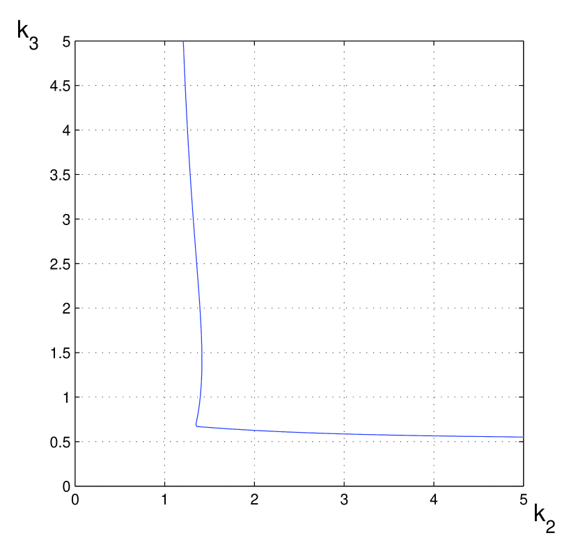
Figure 2: Gain region boundary $\partial\mathcal{K}_{r}$.

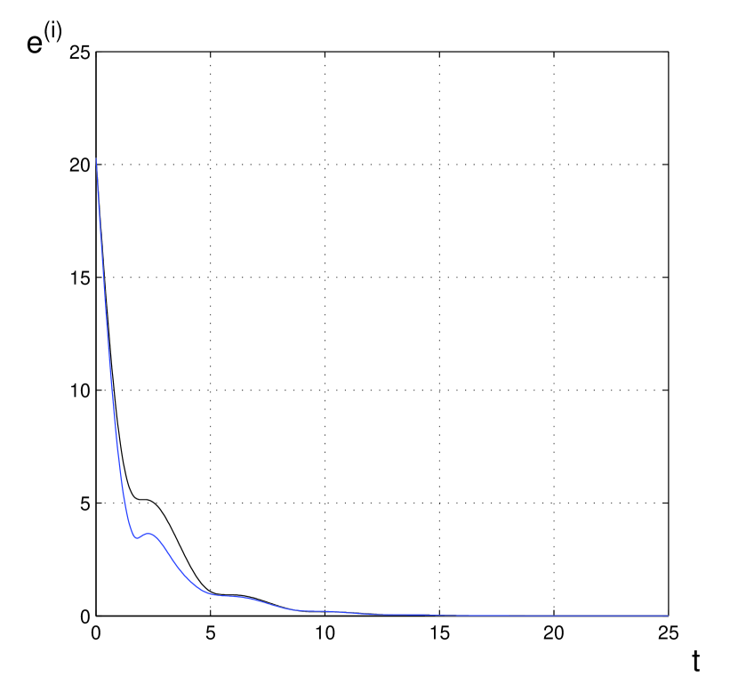
Figure 3: Performance with identical ($e^{(1)}(t)$; black line) and nonidentical ($e^{(2)}(t)$; blue line) gains.

Let us choose following initial conditions:

$$x_{1}(0)=\mathrm{col}(2,-2),x_{2}(0)=\mathrm{col}(-7,3),x_{3}(0)=\mathrm{col}(1,-3).$$

Denote by $e(t)=\sum_{i=1}^{2}\|x_{i}(t)-x_{i+1}(t)\|_{2}$ sum of error norms or disagreement measure; $e^{(1)}(t)$ error in the first case, $e^{(2)}(t)$ error in the second case. Results of 25 sec. simulations are shown on Fig. 3.

Note that consensus vector (11) does not changes for all $(k_{2},k_{3})\in\mathcal{K}$ since subsystem $S_{1}$ is leader.

4.2 Twenty node digraph and nonidentical control

Let us consider digraph shown on Fig.5 consisting of 20 agents $S_{1},\ldots,S_{20}$ described in section 3.1. This dodecahedron-like digraph have Leading Set consisting of dynamic nodes $S_{1},\ldots,S_{10}$ which are connected in directed circle. Let us choose $\nu=k_{1}=k_{2}=\ldots=k_{10}$ and $\mu=k_{11}=k_{12}=\ldots=k_{20}.$ According to Theorem 3 gain $\nu$ should be chosen $\nu>0.5\cdot\cot^{2}(\pi/10)\approx 4.74.$ For faster convergence $\nu$ let us choose $\nu=5.5.$ Simulations show that $\mu$ can be chosen considerably less than $\nu.$ Let us choose $\mu=1,$ and let agents have different initial conditions. Results of numerical simulation show that such nonidentical gain choice provides achievement of consensus. All trajectories of 20 agents on same phase plane are shown on Fig. 5.

Numerical simulations also show that by choosing $\mu=\nu$ and applying Theorem 5 for resulting Laplace matrix one can obtain lower bound approximation $\mu=\nu>4.74.$

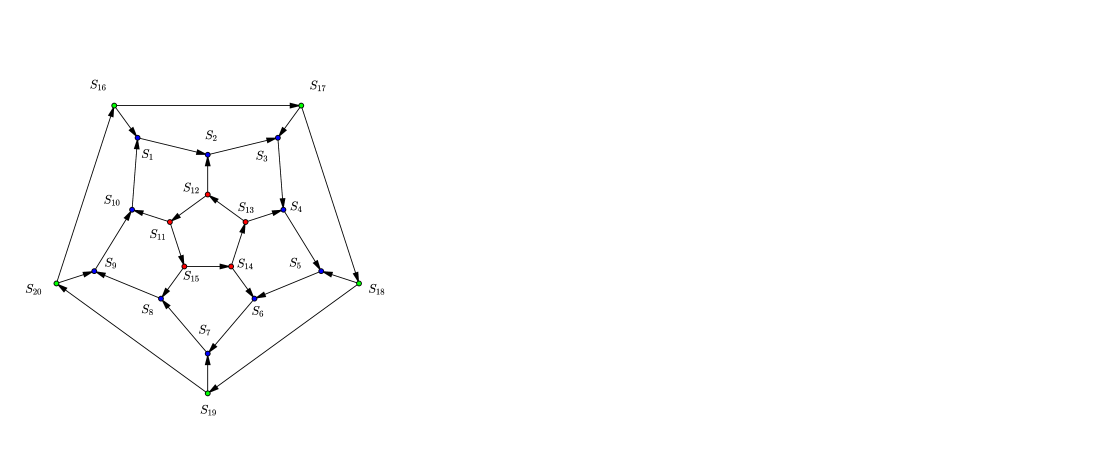
Figure 4: Digraph of 20 agents.

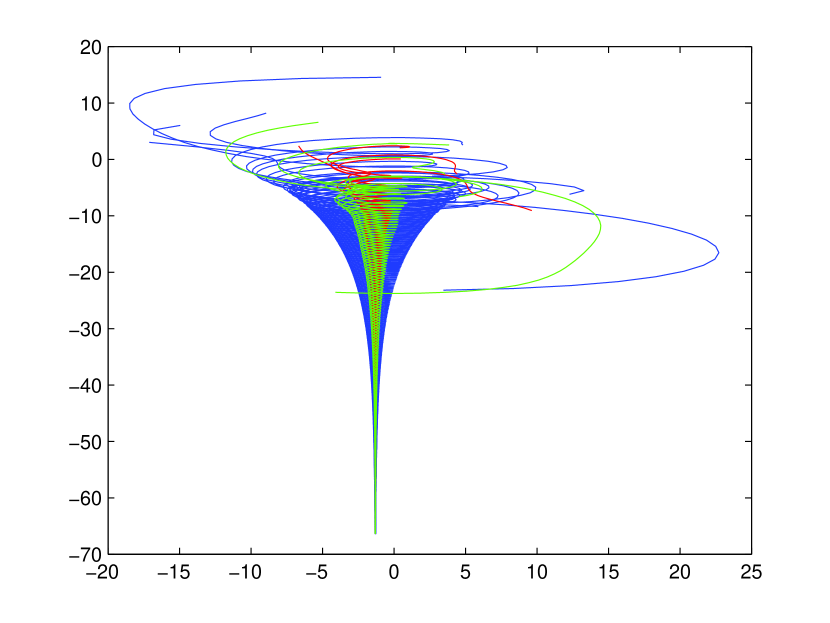
Figure 5: Trajectories of 20 agents on same phase plane. Trajectories of $S_{1},\ldots,S_{10}$ colored blue, $S_{11},\ldots,S_{15}$ colored red, and $S_{16},\ldots,S_{20}$ colored green.

5 Reference remarks

Assumptions of Th. 1 are relaxed in comparison with Th. 2 from [10]. Proof of these results use coordinate tranformation as in [25]. Lemma 2 partially succeeds Th. 3 from [9]. Th. 5 is a trigonometric form of Th. 1 from [26] with different proof.

6 Conclusions

By means of Passification Method sufficient conditions of consensus with identical and nonidentical gains are derived. Synchronous behaviour (consensus vector) is described, it can be affected by nonidentical gains (nonidentity in actuation) within Leading Set. Gain asymptote in growing cycle digraphs which have lowest communication cost for reaching average consensus and consisting of double integrators is studied.

It is rediscovered that cycle digraph connection with nonidentical actuation of nodes causes nonidentical impact on synchronous behaviour. Reachability of synchronization corresponds to positive scalar – common gain. By constructing boundary of sufficient gain region in 3 node digraph it is found that Jordan block of Laplace matrix (which affects transient dynamics) appears in a direction of extremal point. Comparison of dynamics is a subject to a future study. Geometrical interpretations which might be useful in applications and theory were developed.

References

• [1] R. Agaev and P. Chebotarev. The matrix of maximum out forests of a digraph and its applications. Automation and Remote Control, 61(9):1424–1450, 2000.
• [2] R. Agaev and P. Chebotarev. A cyclic representation of discrete coordination procedures. Automation and Remote Control, 73(1):161–166, 2012.
• [3] R. Bellman. Introduction to Matrix Analysis. McGraw-Hill, Inc., 1960.
• [4] S. Boyd, L. Ghaoui, E. Feron, and V. Balakrishnan. Linear Matrix Inequalities in System and Control Theory, volume 15 of Studies in Applied Mathematics. SIAM, 1994.
• [5] B. Brogliato, B. Maschke, R. Lozano, and O. Egeland. Dissipative Systems Analysis and Control/Theory and Applications. Springer, 2007.
• [6] F. Bullo, J. Cortez, and S. Martinez. Distributed control of robotic networks. Princeton Univ. Press, 2009.
• [7] C. Byrnes, A. Isidori, and J. C. Willems. Passivity, feedback equivalence, and the global stabilization of minimum phase nonlinear systems. IEEE Trans. on Autom. Control, 36:1228–1240, 1991.
• [8] P. Chebotarev and R. Agaev. The forest consensus theorem and asymptotic properties of coordination protocols. 4th IFAC Workshop on Distributed Estimation and Control in Networked Systems, Germany, pages 95–101, 2013.
• [9] J. R. Fax and R. M. Murray. Information flow and cooperative control of vehicle formations. IEEE Trans. on Autom. Control, 49:1465–1476, 2004.
• [10] A. Fradkov and I. Junussov. Synchronization of linear object networks by output feedback. 50th IEEE Conf. on Decision and Control and European Control Conf. (CDC-ECC), pages 8188 – 8192, 2011.
• [11] A. L. Fradkov. Quadratic lyapunov functions in the adaptive stabilization problem of a linear dynamic plant. Siberian Math J, 2:341–348, 1976.
• [12] A. L. Fradkov. Passification of nonsquare linear systems and feedback yakubovich-kalman-popov lemma. Eur. J. Control, (6):573–582, 2003.
• [13] I. Gutman and D. Vidovic. The largest eigenvalues of adjacency and laplacian matrices, and ionization potentials of alkanes. Indian J. Chem., 41A:893–896, 2002.
• [14] F. Harary. Graph Theory. Addison–Wesley, Reading, MA., 1969.
• [15] I. Herman, D. Martinec, Z. Hurak, and M. Shebek. Scaling of transfer functions in vehicular platoons: the role of asymmetry disputed. http://arxiv.org/abs/1410.3943, 2014.
• [16] R. Horn and C. Johnson. Matrix analysis. Cambridge University Press, 1990.
• [17] P. Kokotovic and M. Arcak. Constructive nonlinear control: a historical perspective. survey paper. Automatica, 37:637–662, 2001.
• [18] P. Kokotovic and H. Sussmann. A positive real condition for global stabilization of nonlinear systems. Systems and Control Letters, 19:177–185, 1989.
• [19] Z. K. Li, Z. S. Duan, G. R. Chen, and L. Huang. Consensus of multi-agent systems and synchronization of complex networks: A unified viewpoint. IEEE Trans. On Circuits And Systems-I: Reg. Papers, 57(1):213–224, 2010.
• [20] M. Marcus and H. Minc. A Survey of Matrix Theory and Matrix Inequalities. Allyn and Bacon, Inc., Boston, 1964.
• [21] M. Mesbahi and M. Egerstedt. Graph Theoretic Methods in Multiagent Networks. Princeton Univ. Press, 2010.
• [22] R. Olfati-Saber, J. Fax, and R. Murray. Consensus and cooperation in networked multi-agent systems. Proc. IEEE, 95(1):215–233, January 2007.
• [23] W. Ren, R. W. Beard, and E. M. Atkins. A survey of consensus problems in multi-agent coordination. Proc. of American Control Conference, Oregon, pages 1859–1864, 2005.
• [24] C. Reynolds. Flocks, herds, and schools: A distributed behavioral model. Computer Graphics, 21(4):25–34, July 1987.
• [25] C. Yoshioka and T. Namerikawa. Observer-based consensus control strategy for multi-agent system with communication time delay. Proceedings of IEEE MSC-2008, San-Antonio, USA, pages 1037–1042, 2008.
• [26] W. Yu, G. Chen, and M. Cao. Some necessary and sufficient conditions for second-order consensus in multi-agent dynamical systems. Automatica, 46:1089–1095, 2010.
• [27] H. Zhang, F. L. Lewis, and A. Das. Optimal design for synchronization of cooperative systems: State feedback, observer and output feedback. IEEE Trans. on Autom. Control, 56(8):1948–1952, August 2011.