THE EFFECT OF TEMPERATURE EVOLUTION ON THE INTERIOR STRUCTURE OF H₂O-RICH PLANETS

Abstract

For most planets in the range of radii from 1 to 4 R_⊕, water is a major component of the interior composition. At high pressure H₂O can be solid, but for larger planets, like Neptune, the temperature can be too high for this. Mass and age play a role in determining the transition between solid and fluid (and mixed) water-rich super-Earth. We use the latest high-pressure and ultra-high-pressure phase diagrams of H₂O, and by comparing them with the interior adiabats of various planet models, the temperature evolution of the planet interior is shown, especially for the state of H₂O. It turns out that the bulk of H₂O in a planet’s interior may exist in various states such as plasma, superionic, ionic, Ice VII, Ice X, etc., depending on the size, age and cooling rate of the planet. Different regions of the mass-radius phase space are also identified to correspond to different planet structures. In general, super-Earth-size planets (isolated or without significant parent star irradiation effects) older than about 3 Gyr would be mostly solid.

1 INTRODUCTION

The catalog of observed extrasolar planets now includes more than 1700 members, and more than 1100 planets have been observed transiting their parent stars (Rein, 2014). Transiting planets are particularly valuable for comparative planetology because they provide the planet’s radius, as well as the inclination angle of the planet’s orbit with respect to the line of sight. When combined with the mass determined from radial velocity measurements, the mean density of the planet can be determined.

Super-Earths, massive terrestrial exoplanets within the range of $1M_{\oplus}\lesssim M\lesssim 15M_{\oplus}$, are now observed to be relatively common by Doppler shift surveys and transiting observations. The currently discovered super-Earth extrasolar planets suggest diversity among their interior structure and composition – some being very dense (such as CoRoT-7b (Leger et al., 2009; Queloz et al., 2009)), and the others seem much less so (such as GJ 1214b (Charbonneau et al., 2009)). Moreover, among the Super-Earths, it has been speculated that some of them may contain more than 10$\%$ $\sim$ 15$\%$ of H₂O by weight, the so-called water planets (or H₂O-rich planets). The candidates of those water planets include GJ 1214b, Kepler-22b, Kepler-68b, and Kepler-18b. There is no exact definition of H₂O-rich planets; however, based on the implication from the planet formation theory, we could propose the range of anywhere between 25$\%$ and 75$\%$ mass fraction of H₂O (Marcus et al., 2010). A value of 100$\%$ H₂O would be unlikely because silicate, metal and H₂O would tend to be mixed in proportions in the protoplanetary nebula.

The H₂O-rich planets could be roughly divided into two types:

1. planets with their bulk H₂O in the solid phase, or solid H₂O-rich planets

2. planets with their bulk H₂O in the fluid phase (including molecular, ionic, or plasma phases), like Uranus and Neptune in our solar system but smaller, the so-called mini-Neptunes

It is of particular interest to distinguish between the two types. Furthermore, it would be interesting to know if a planet could transition from one type to the other through thermal evolution, such as the heating or cooling of its interior. The division between the two types depends on the phase diagram of H₂O and the mass, the bulk composition, and the interior temperature profile of the planets being considered. Thus the goal of this paper is to identify regions and boundaries on the mass-radius (M-R) diagram in order to distinguish planets with different phases of H₂O within their interior and to understand how the phases of H₂O in the interior could change as planets cool through aging.

The baseline interior structure model is taken from Zeng & Sasselov (2013) and Zeng & Seager (2008). Here we simplify a H₂O-rich planet to a fully differentiated planet composed of two distinct layers: a MgSiO₃ (silicate) core and an H₂O mantle. More detailed three-layer model including the metallic iron is available online,  http://www.astrozeng.com, as a user-friendly interactive tool.

2 H₂O PHASE DIAGRAM

The low-pressure and low-temperature phase diagram of H₂O is notorious for its rich and complex structure. At pressures below $\sim 3$GPa and temperatures below $\sim 500$ K, the hydrogen bond is mostly responsible for the diversity of phases. However, the high-pressure and high-temperature phases of H₂O appear to be similarly complex (the transitions between $\sim$1000 K and 4000 K), as one approaches the plasma phase of H₂O and its dissociation at higher temperatures. The interplay between oxygen atom packing and proton mobility seem to account for much of that complexity.

The pressure-temperature plot (Figure 1) shows different H₂O phases in the pressure-temperature regime of interest. The phase boundaries are drawn approximately and are obtained either through experiments (summarized by Chaplin (2012)) or by first-principle ab initio simulations (French et al., 2009; Redmer et al., 2011). The region marked ”molecular fluid” lies above the critical point of H₂O ($T_{c}=$ 647 K, $P_{c}=$ 22 MPa), i.e., supercritical fluid. The transitions between molecular, ionic, and plasma fluids are gradual (Redmer et al., 2011).

Various structures of Ice XI have been postulated to exist at ultra-high pressure beyond Ice X by ab initio simulations. Those structures are yet to be confirmed by experiments (Hermann et al., 2012; Militzer & Wilson, 2010).

The phase above (higher temperature) the previously known solid forms of Ice VII and Ice X is the ”superionic” H₂O. Superionic solids are known previously for other materials, e.g., PbF₂ and AgI. However, for H₂O the phase was first predicted theoretically (Cavazzoni et al., 1999; Goldman et al., 2005) and confirmed later by experiments (Ji et al., 2011). In particular, superionic H₂O is characterized by a preserved stable oxygen lattice and mobile protons. The ionic conductivity of protons is primarily responsible for the electrical conductivity. The properties of superionic H₂O may have remained as an exotic bit of high-pressure physics, if not for the fact that the pressure-temperature profiles of some super-Earths seem to pass close to the triple point between fluid, superionic, and high-pressure ice phases of H₂O.

3 THERMAL EVOLUTION OF H₂O-RICH PLANET

The thermal evolution models of a 50wt$\%$ MgSiO₃-50wt$\%$ H₂O planet, of masses 2, 6, 18.5 $M_{\oplus}$, each of age 2, 4.5, and 10 Gyr (billion years), are considered here. The equation of state (EOS) is from Zeng & Sasselov (2013). Figure 2 illustrates one example of the models.

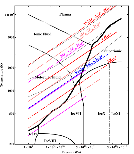
Figure 1: Pressure-temperature profiles of H₂O-layer of various super-Earth models of different ages, over the H₂O phase diagram. The thick black curve is the solid-fluid boundary (melting curve). Three thin black curves are the adiabats calculated from Vazan et al.’s (2013) EOS for comparison. The blue dot-dashed line shows the adiabat for Kepler-68b at the estimated age of 6.3 Gyr (Gilliland et al., 2013). The nine thermal gradient models as well as the Kepler-68b model are tabulated in Table 1. The surface pressure of each model is defined as 1 bar ($10^{5}$ Pa), far beyond the left limit of the diagram. The dotted line indicates the continuous transition from molecular to ionic fluid due to dissociation (more than $20\%$ of the water molecules dissociated), the dashed line indicates the continuous transition from ionic to plasma fluid due to ionization (electronic conductivity $>100\Omega^{-1}$ cm^-1) in the dense fluid. The boundary between Ice X and Ice XI is still subject to experimental verification.

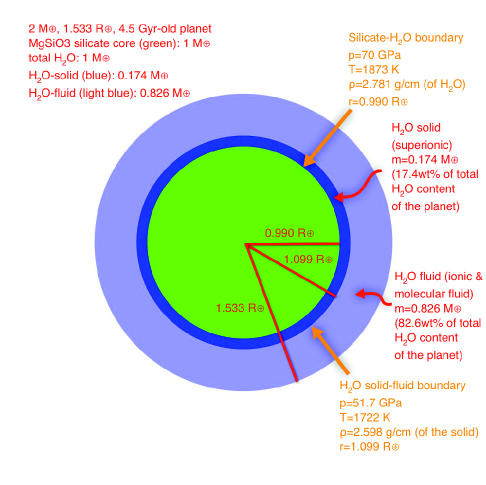
Figure 2: Two-layer super-Earth of 2 $M_{\oplus}$ and 1.5 $R_{\oplus}$ at 4.5 Gyr. The interior temperature profile of the H₂O-layer of this model is represented by the solid magenta curve in Figure 1.

Figure 1 shows the thermal gradients of the models. The three red curves are the models of 18.5 $M_{\oplus}$ and 2.7 $R_{\oplus}$ (large super-Earth, similar to Neptune in terms of mass), of three different ages (2, 4.5 and 10 Gyr). The three pink curves are the models of 6 $M_{\oplus}$ and 2 $R_{\oplus}$ (midsize super-Earth), and the three magenta curves are the models of 2 $M_{\oplus}$ and 1.5 $R_{\oplus}$ (small super-Earth, slightly bigger than Earth). Irradiation by the parent star can have a great effect on the results; most of the super-Earths known today are close to their parent stars. Such planets will stay warm longer. This could increase the length of time they are habitable. For example, the equilibrium temperature of Kepler-68b is estimated to be around 1200 K (Gilliland et al., 2013), which would have retarded the cooling of the planet from the surface down to about 10 GPa depth at its current estimated age of 6.3 Gyr.

In order to obtain the initial thermal states to scale from, we have two options. Since we know a lot more details of interior thermal states of solar system planets, compared to exoplanets, it is a good starting point of our model. Most of these H₂O-rich planets lie in between Neptune and Earth in terms of their mass and radius; thus we could either scale up from Earth, or scale down from Neptune. Earth is not a H₂O-rich planet, so it would make more sense to scale from Neptune. Therefore, we start with Neptune’s interior adiabat at the current of age of 4.5 Gyr. We fit an analytical line in log$p$-log$T$ space to Neptune’s adiabat Redmer et al. (2011). Then we scale the adiabat to planets of different mass and radius according to essentially their core-mantle boundary temperature T1 and pressure p1, by looking at the similar scaling law of planets in our solar system. Finally, we evolve this scaled adiabat backward or forward to different ages using the rheology law derived in Equation (2). In this way, we derive a simple analytical model of planet’s interior temperature as a function of its age and pressure: Equation (1), and Table 1 for a few cases.

Comparing Figure 2 to the same model (2 $M_{\oplus}$, 4.5 Gyr) represented by the solid magenta curve in Figure 1, one can see that a small segment of the $P-T$ curve toward the right end (the region near the H₂O-silicate boundary) would correspond to a significant mass fraction of H₂O inside the planet because the pressure scale is logarithmic in the diagram. A simple rule of thumb is that, for the H₂O below the depth of $50\%$ p1 (half the H₂O-silicate boundary pressure), it contains $\sim 40\%$ the total H₂O mass, and for the H₂O below $10\%$ p1 (one-tenth the H₂O-silicate boundary pressure), it contains $>80\%$ H₂O mass. For example, the mass of the solid H₂O in the 2 $M_{\oplus}$ 4.5 Gyr-old planet is 0.174 $M_{\oplus}$; this is the model illustrated in Figure 2.

Table 1: Table of the Pressure-Temperature Profiles of H₂O layer

Model 1: 2.001 $M_{\oplus}$, 1.533 $R_{\oplus}$
$p$ (GPa)	Mass Fraction	Depth (km)	Density (g cm-3)	$T$ (K) (2 Gyr)	$T$ (4.5 Gyr)	$T$ (10 Gyr)
0.0001	0	0	0.918	101	45	20.3
1	0.0236	101	1.33	1300	577	260
2	0.0466	189	1.36	1570	700	315
5	0.113	410	1.66	2030	902	406
10	0.215	740	1.83	2460	1090	492
20	0.397	1310	2.09	2980	1320	596
50	0.807	2700	2.58	3840	1710	768
70	1	3460	2.78	4210	1870	843
Model 2: 5.966 $M_{\oplus}$, 2.050 $R_{\oplus}$
$p$ (GPa)	Mass Fraction	Depth (km)	Density (g cm-3)	$T$ (2 Gyr)	$T$ (4.5 Gyr)	$T$ (10 Gyr)
0.0001	0	0	0.918	128	56.9	25.6
1	0.00855	60.7	1.33	1640	730	328
2	0.017	114	1.36	1990	884	398
5	0.0418	247	1.66	2560	1140	513
10	0.0817	448	1.83	3110	1380	621
20	0.157	798	2.09	3760	1670	753
50	0.356	1660	2.58	4850	2160	970
70	0.472	2150	2.78	5330	2370	1070
100	0.625	2820	3.01	5880	2610	1180
200	1	4690	3.59	7120	3170	1420
Model 3: 18.52 $M_{\oplus}$, 2.687 $R_{\oplus}$
$p$ (GPa)	Mass Fraction	Depth (km)	Density (g cm-3)	$T$ (2 Gyr)	$T$ (4.5 Gyr)	$T$ (10 Gyr)
0.0001	0	0	0.918	169	75.2	33.9
1	0.00263	33.7	1.33	2170	965	434
2	0.00525	63.1	1.36	2630	1170	526
5	0.013	138	1.66	3390	1510	678
10	0.0258	249	1.83	4110	1830	822
20	0.0506	447	2.09	4980	2210	996
50	0.121	933	2.58	6420	2850	1280
70	0.165	1210	2.78	7040	3130	1410
100	0.227	1600	3.01	7770	3460	1550
200	0.41	2690	3.59	9420	4190	1880
500	0.813	5130	4.75	12100	5400	2430
700	1	6400	5.33	13300	5920	2670
Kepler-68b Model: 8.3 $M_{\oplus}$, 2.31 $R_{\oplus}$
$p$ (GPa)	Mass ($M_{\oplus}$)	Radius ($R_{\oplus}$)	Density (g cm-3)	$T$ (2 Gyr)	$T$ (6.3 Gyr)	$T$ (10 Gyr)
0.0001	8.32	2.31	0.918	146	46.2	29.1
1	8.29	2.3	1.33	1870	592	373
2	8.26	2.29	1.36	2260	718	452
5	8.17	2.28	1.66	2910	925	583
10	8.03	2.25	1.83	3530	1120	706
20	7.76	2.2	2.09	4280	1360	856
50	7.04	2.07	2.58	5510	1750	1100
70	6.6	2	2.78	6050	1920	1210
100	6	1.9	3.01	6680	2120	1340
200	4.42	1.61	3.59	8100	2570	1620
300	3.3	1.37	4.04	9060	2880	1810
355	2.84	1.25	4.26(H2O)	9490	3010	1900
355	2.84	1.25	7.06(MgSiO3)	Core-mantle boundary
600	1.29	0.939	8.10
900	0.148	0.443	9.08	MgSiO3 post-perovskite (ppv)
900	0.148	0.443	9.29	ppv dissociates to MgO and MgSi2O5 (Umemoto & Wentzcovitch, 2011)
1000	0	0	9.61	center of the planet

The thermal evolution models (the nine thick $P-T$ profiles in Figure 1) are calculated by the following equation:

$$T[\tau,p_{1}][p]=10^{-2.15}\times\frac{4.5~{}\textrm{Gyr}}{\tau}\times\sqrt{\frac{p_{1}}{1~{}\textrm{Pa}}}\times\left(\frac{p}{p_{1}}\right)^{0.277}$$ (1)

Here $p_{1}$ is the pressure (in Pa) at the H₂O-silicate boundary (i.e., the pressure at the bottom of the H₂O layer). $\tau$ is the age of the planet in units of billions of years (Gyr); $p$ is an arbitrary pressure within the H₂O layer; and $T[\tau,p_{1}][p]$ calculates the corresponding temperature (in Kelvin). The cooling rate can also be influenced by the phase of the H₂O in the mantle (different Rayleigh numbers, different convection speeds in different phases, etc.). Equation (1) assumes a constant cooling rate for all solid phases of H₂O. It also assumes that the cooling of the planet is primarily controlled by the viscosity of the solid part of the planet. This assumption is robust as long as the heat transfer mechanism outward is dominated by the temperature-dependent viscosity-driven solid-state convection in the mantle or core. As long as the viscosity has an exponential dependence on temperature, the scaling law is the same. In some cases, mainly in the early evolution, solid H₂O part does not yet exist; however, the silicate core of the planet still remains solid. So the assumption here is that the cooling rate of the planet is still controlled by the bottleneck, which is how fast the solid part could convect out heat.

Phase transitions from fluids to solids are generally exothermic and release energy (latent heat); thus it could also have an influence on the temperature evolution when the H₂O in the planet interior transitions from fluid to solid phase, retarding the cooling at the phase transition boundary. However, current experiments could not reach that pressure-temperature regime to measure the latent heat of phase transition yet, and the theoretical calculation has large uncertainties. Therefore, we choose to ignore the latent heat for now.

The temperature gradient in the fluid part of the H₂O layer should be adiabatic. Because the viscosity of a fluid is small, any deviation from adiabat would be quickly offset by convection. For the solid part of the H₂O layer, as pointed out by Fu et al. (2010); O’Connell & Hager (1980), the bulk H₂O ice mantle would exhibit a whole-mantle convection without partitioning inside, so it is reasonable to approximate the thermal gradient as an adiabat also.

Equation (1) represents a family of adiabats, characterized by the same slope in log$P$-log$T$ plot, scaling to different characteristic interior temperatures ($T_{i}$).

Equation (1) is obtained by downscaling the pressure-temperature profile of the interior of Neptune (Redmer et al., 2011) according to the pressure at the H₂O-silicate boundary, and assuming the cooling of the planet is primarily controlled by the rheology (viscosity) of the solid part of the planet (the bottom solid H₂O layer, and predominately the silicate core underneath), that is, by how strong the solid part of the planet can convect and transport the heat out. Following the argument in Turcotte & Schubert (2002), assuming an exponential dependence of the viscosity on the inverse of temperature

$$\mu=\mu_{r}\times\textrm{exp}(\frac{E_{a}}{RT})$$ (2)

(where $\mu_{r}$ is a constant of proportionality, $E_{a}$ is the activation energy, and R is the gas constant) and including the contribution of the radioactive heat sources, one could derive a result showing that the characteristic interior temperature $T_{i}$ of a planet is, to the first order, inversely proportional to its age. Vazan et al. (2013) modeled the evolution of giant and intermediate-mass planets. Three adiabats (thin curves in Figure 1) calculated from their H₂O EOS in the region of validity (private communication) are shown to match quite well with our $P-T$ profiles’ gradients, confirming the validity of Equation (1). However, it should be noted that Equation (1) should only be taken as a qualitative order-of-magnitude estimate because the actual thermal gradient may depend on many other factors, such as different abundance of the radioactive elements in the interior, different initial thermal states, and the surface boundary conditions of the planet.

The slope of the adiabats are in general shallower than the melting curve, suggesting that for high enough pressure, the adiabat trend would usually intersect the melting curve and result in the high-pressure ice phases or superionic phase usually sitting at the bottom of the fluid phase but not the other way around.

4 IMPLICATIONS AND IMPORTANCE OF THE MODELS

Comparing Equation (1) to the H₂O phase diagram shows that, as a H₂O-rich planet ages and cools down, its bulk H₂O may undergo phase transition, first from fluid phases to superionic phase, then from superionic phase to high-pressure ices. The timing of these phase transitions would depend on the pressure $p_{1}$ at the bottom of the H₂O layer, the initial thermal state of the planet, the abundance of radioactive elements in the interior, and so on. These phase transitions may affect the radius of the planet only slightly, but they may significantly affect the interior convective pattern of the planet and also the global magnetic field of the planet, which results from the dynamo action inside the planet, which in turn depends on the strength of convection, differential rotation, and the electrical conductivity of the convective layer. The existence of the superionic layer is especially favorable for the dynamo action to take place, speculated as probably what is happening in Uranus and Neptune now. As pointed out by Stanley & Bloxham (2006) and Redmer et al. (2011), the nondipole magnetic fields of Uranus and Neptune are presumably due to the presence of a conductive superionic H₂O shell surrounding the solid core acting as a dynamo. Such a scenario could similarly exist on other planets that possess such an electrically conductive region (superionic, ionic or plasma phase) of H₂O or other species. The implication of the existence of a global magnetic field on the habitability of the planet is also significant, as has been suggested by some people (Ziegler & Stegman, 2013; Bradley, 1994), and manifested by our own Earth, that the existence of the magnetic field of Earth shortly after its formation is intimately tied to the origin of life on Earth because it shields the harmful UV radiation from the host star and may have something to do with the origin of chirality of biomolecules such as RNA and protein.

5 MASS RADIUS DIAGRAM AND H₂O PHASE REGIONS

The mass fraction of H₂O out of the total planet mass is varied from 25$\%$ to 75$\%$ in the two-layer model, to show the correspondence between different regions of the $M-R$ diagram to different phases of near-bottom H₂O for planets of different ages (Figure 3).

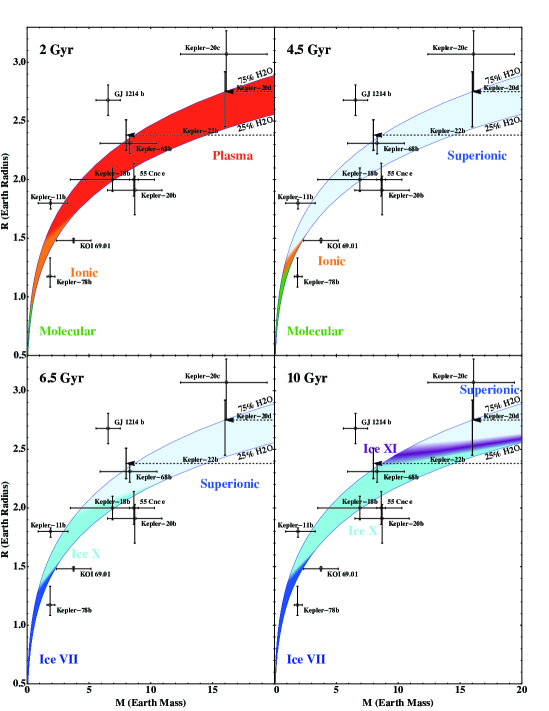
Figure 3: Mass-radius diagram as a function of cooling age corresponding to different phases of H₂O near the H₂O-silicate boundary, for H₂O-silicate planets with H₂O mass fraction from 25$\%$ to 75$\%$, of different ages (2, 4.5, 6.5, and 10 Gyr). Exoplanets close to the region of interest are shown, as well as recently discovered KOI 69.01 (Ballard et al., 2013) and Kepler-78b (Pepe et al., 2013).

The various colored regions in Figure 3 could be compared to the measured masses, radii and ages of observed exoplanets to help us understand the phases of H₂O of those planets within this mass range and its implications for planet thermal evolution, convection, magnetic field and habitability. The transport and mixing of volatiles will be different in planets with solid H₂O mantle rather than fluid (Levi et al., 2013), and that will affect the composition of their atmospheres. For Kepler-68b, there is an accurate age measurement of $6.3\pm 1.7$ Gyr from asteroseismology (Gilliland et al., 2013), which when combined with our model would indicate the presence of solid superionic H₂O in its interior.

One thing to point out is that in our model we have not considered the possible existence of a thick gaseous envelope/atmosphere (such as H/He) that could overlie the H₂O layer and increase the observed radii of planets. This gaseous envelope might act as a thermal blanket that would slow the cooling of the planet (Stevenson, 2013), and instead of interior temperature $T_{i}\sim\tau^{-1}$, it will go as $T_{i}\sim\tau^{-1/3}$ or even slower. However, because of its low density, it would not increase the interior pressure significantly. We hope to explore this aspect more in future research.

6 CONCLUSION

We use simple two-layer (silicate-core and H₂O-mantle) planet models to understand the thermal evolution of H₂O-rich planets. The interior pressure versus temperature profiles of nine specific models are plotted over the H₂O phase diagram to show the existence of difference phases of H₂O with the thermal evolution of the planets.

The cooling of a H₂O-rich planet results in its bulk H₂O content transitioning first from fluid phases to superionic phase, and later from the superionic phase to high-pressure ices. These transformations may have a significant effect on the interior convective pattern and also the magnetic field of such a planet, but they may only affect the overall radius slightly.

Different regions in the mass-radius phase space are identified to correspond to different phases of H₂O near the bottom of the H₂O layer in a H₂O-rich planet, which are usually representative of the bulk H₂O in the entire planet (because of the logarithmic pressure scale, a small portion of $P-T$ profile toward the right end would correspond to a considerable amount of H₂O by mass). In general, super-Earth-size planets (isolated or without significant parent star irradiation effect) older than about 3 Gyr would be mostly solid. These regions could be compared to observation, to sort the exoplanets into various H₂O-rich planet categories, and help us understand the exoplanet population, composition, and interior structure statistically.

The authors are very grateful to Richard O’Connell, Morris Podolak, Jerry Mitrovica, Jeremy Bloxham, Stein Jacobsen, Michail Petaev, Amit Levi, Eric Lopez and David Stevenson for their valuable comments and suggestions and fruitful discussions, and Allona Vazan and Attay Kovetz in particular, for sharing their data of the H₂O EOS with us to compare with our model. This work has been supported in part by the Harvard Origins of Life Initiative.

References

- Ballard et al. (2013) Ballard, S., Huber, D., Chaplin, W., et al. 2013, ApJ, submitted
- Bradley (1994) Bradley, D. 1994, Science, 264, 908
- Cavazzoni et al. (1999) Cavazzoni, C., Chiarotti, G. L., Scandolo, S., et al. 1999, Science, 283, 44
- Chaplin (2012) Chaplin, M. 2012, Water Phase Diagram, http://www.lsbu.ac.uk/water/phase.html#bb
- Charbonneau et al. (2009) Charbonneau, D., Berta, Z. K., Irwin, J., et al. 2009, Nature, 462, 891
- French et al. (2009) French, M., Mattsson, T. R., Nettelmann, N., & Redmer, R. 2009, Phys. Rev. B, 79, 054107
- Fu et al. (2010) Fu, R., O’Connell, R. J., & Sasselov, D. D. 2010, The Astrophysical Journal, 708, 1326
- Gilliland et al. (2013) Gilliland, R. L., Marcy, G. W., Rowe, J. F., et al. 2013, The Astrophysical Journal, 766, 40
- Goldman et al. (2005) Goldman, N., Fried, L. E., Kuo, I.-F. W., & Mundy, C. J. 2005, Phys. Rev. Lett., 94, 217801
- Hermann et al. (2012) Hermann, A., Ashcroft, N. W., & Hoffmann, R. 2012, Proceedings of the National Academy of Sciences, 109, 745
- Ji et al. (2011) Ji, M., Umemoto, K., Wang, C.-Z., Ho, K.-M., & Wentzcovitch, R. M. 2011, Phys. Rev. B, 84, 220105
- Leger et al. (2009) Leger, A., Rouan, D., Schneider, J., et al. 2009, Astronomy and Astrophysics, 506, 287
- Levi et al. (2013) Levi, A., Sasselov, D., & Podolak, M. 2013, The Astrophysical Journal, 769, 29
- Marcus et al. (2010) Marcus, R., Sasselov, D., Stewart, S., & Hernquist, L. 2010, The Astrophysical Journal Letters, 719, L45
- Militzer & Wilson (2010) Militzer, B., & Wilson, H. F. 2010, Phys. Rev. Lett., 105, 195701
- O’Connell & Hager (1980) O’Connell, R. J., & Hager, B. H. 1980, Proc. Int. School of Physics Enrico Fermi, course 78, ed. A. M. Dziewonski and E. Boschi (Amsterdam: North- Holland), 270
- Pepe et al. (2013) Pepe, F., Collier Cameron, A., Latham, D. W., et al. 2013, ArXiv e-prints
- Queloz et al. (2009) Queloz, D., Bouchy, F., Moutou, C., Hatzes, A., & Hébrard, G. 2009, Astronomy and Astrophysics, 506, 303
- Redmer et al. (2011) Redmer, R., Mattsson, T. R., Nettelmann, N., & French, M. 2011, Icarus, 211, 798
- Rein (2014) Rein, H. 2014, Open Exoplanet Catalogue, http://github.com/hannorein/open_exoplanet_catalogue/
- Stanley & Bloxham (2006) Stanley, S., & Bloxham, J. 2006, Icarus, 184, 556
- Stevenson (2013) Stevenson, D. J. 2013, Planets, Stars and Stellar Systems (Springer), 195–221
- Turcotte & Schubert (2002) Turcotte, D., & Schubert, G. 2002, Geodynamics, 2nd ed (Cambridge University Press), 325–326
- Umemoto & Wentzcovitch (2011) Umemoto, K., & Wentzcovitch, R. M. 2011, Earth and Planetary Science Letters, 311, 225
- Vazan et al. (2013) Vazan, A., Kovetz, A., Podolak, M., & Helled, R. 2013, Monthly Notices of the Royal Astronomical Society, 434, 3283
- Zeng & Sasselov (2013) Zeng, L., & Sasselov, D. 2013, Publications of the Astronomical Society of the Pacific, 125, pp. 227
- Zeng & Seager (2008) Zeng, L., & Seager, S. 2008, Publications of the Astronomical Society of the Pacific, 120, 983
- Ziegler & Stegman (2013) Ziegler, L. B., & Stegman, D. R. 2013, Geochemistry, Geophysics, Geosystems, 14, 4735