³He-R: A Topological $s^{\pm}$ Superfluid with Triplet Pairing

Abstract

We show that when spin and orbital angular momenta are entangled by spin-orbit coupling, this transforms a topological spin-triplet superfluid/superconductor state, such as ³He-B, into a topological $s^{\pm}$ state, with non-trivial gapless edge states. Similar to ³He-B, the $s^{\pm}$ state also minimizes on-site Coulomb repulsion for weak to moderate interactions. A phase transition into a topological $d$-wave state occurs for sufficiently strong spin-orbit coupling.

I Introduction

Topological states of matter, including topological insulators, superconductors and superfluids are of great current interestVolovik (2003); Schnyder et al. (2008); Ryu et al. (2010); Qi and Zhang (2011). Spin-orbit coupling plays a key role in driving the non-trivial topology of 3D topological insulators, and a topological superconducting phase (spinless $p+ip$) can also be induced by proximity effect between a conventional $s$-wave superconductor and a material with strong spin-orbit coupling, such as a topological insulator Fu and Kane (2008); Sau et al. (2010); Oreg et al. (2010). In this paper, we will show that a topological $s^{\pm}$ state can also be generated using the converse effect of spin-orbit coupling on a $p$-wave condensate.

To illustrate this physics, we introduce a toy model, describing 2D ³He-B with an additional tunable Rashba coupling. This tunable coupling term is absent in real He-3, but the model provides a simple and pedagogical example of the effect of strong spin-orbit coupling on a topological superconductor that may be generalized to a larger class of superconductors, such as Sr₂RuO₄ Rice and Sigrist (1995); Ishida et al. (1998); Luke et al. (1998); Mackenzie and Maeno (2003), in which either spin, or some other internal degree of freedom may become entangled with the momentum-space structure of the condensate. ³He-B is the canonical example of a topological superfluidVollhardt and Wölfle (2013). An early theory of p-wave pairing applicable to the B-phase of He-3B, was proposed by Balian and Werthammer in 1963Balian and Werthamer (1963), prior to its experimental discovery in the 1970’s Osheroff (1997); Leggett (1975); Wheatley (1975); Vollhardt and Wölfle (2013). While the anisotropic $p$-wave nature of its pairing due to the fermionic hard-core repulsion was predicted early on Balian and Werthamer (1963); Anderson and Morel (1961); the underlying topological character of the wavefunction, together with its gapless Majorana edge states were only pointed out in 2003 by Volovik Volovik (2003, 2009a, 2009b); more recent works have connected He-3B with a much more general class of topological superfluidsQi et al. (2009); Wu and Sauls (2013).

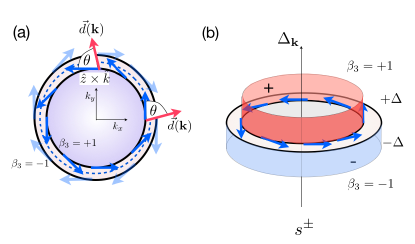
Figure 1: (a) With Rashba coupling, the 2D Fermi surface is split into two with opposing helicities $\beta_{3}=\pm 1$. The relative orientation of the helicity vector $\hat{z}\times\hat{k}$ and the triplet pairing $\hat{d}({\bf k})$ vector is $\theta$. (b) In the superfluid ³He-R condensate, the gap is maximized when the helicity and $\hat{d}({\bf k})$ vectors align ($\theta=0$), developing an $s^{\pm}$ gap function with opposite signs on the two Fermi surfaces.

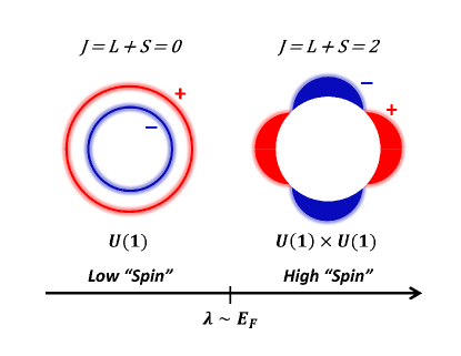
Figure 2: A phase transition from the $s^{\pm}$ state into a $d$-wave state occurs when the spin-orbit interaction is sufficiently strong to lift one of the helical bands above $E_{F}$.

³He-B is a $p$-wave superfluid with unbroken time-reversal symmetry. Although the underlying gap functions contain nodes, the combination of orthogonal spin channels ($\sigma_{x,y,z}$) causes the various p-wave gaps to add in quadrature, hiding one-another’s nodes and giving rise to a fully gapped excitation spectrum. In the absence of spin-orbit coupling, the spin ($S$) and angular momentum ($L$) of the Cooper pairs are well-defined quantum numbers. However, spin-orbit coupling entangles $L$ and $S$, and only the total angular momentum, $J=L+S$, is well-defined. We show that when orbital and spin angular momentum become mixed, a $p$-wave superfluid is transformed into a topological $s^{\pm}$ ($J=1-1=0$) or a nodal $d$-wave ($J=1+1=2$) superfluid, as the spin-orbit coupling strength is increased.

Our analysis includes the $U(1)$ rotational degree of freedom between the spin-orbit, $\hat{n}_{{\bf k}}$, and superconducting $\hat{d}_{{\bf k}}$ vectors, which was ignored in previous works Frigeri et al. (2004); Sato and Fujimoto (2009); Tanaka et al. (2010) on non-centro-symmetric superconductors, where it was assumed that $\hat{n}_{{\bf k}}$ and $\hat{d}_{{\bf k}}$ are always parallel due to strong spin-orbit coupling. Here, we show that the strong Coulomb repulsion breaks the alignment of $\hat{n}_{{\bf k}}$ and $\hat{d}_{{\bf k}}$, and the mixing of $s$ and $d$-wave spin-singlet pairing, with the $p$-wave spin-triplet pairing naturally arises from the in-phase and counter-phase rotation of $\hat{n}_{{\bf k}}$ and $\hat{d}_{{\bf k}}$ respectively.

Specifically, our key results are:

1. At weak to moderate spin-orbit coupling, the ground-state of isotropic ³He-B adiabatically transforms into a “low-spin” $J=1-1=0$ s-wave condensate, made up of two fully gapped spin-polarized Fermi surfaces of opposite pairing phase. This state retains the topological character of its p-wave parent, forming an “$s^{\pm}$” state with topologically protected gapless edge states.

2. In the presence of strong spin-orbit coupling ($\lambda_{{\bf k}}\approx\mu$), the system undergoes a topological phase transition into a “high-spin” topological $d$-wave state with angular momentum ($J=1+1=2$). We note that the $d$-wave state has been discussed in the context of neutron stars by earlier groups David Pines (1985); Hoffberg et al. (1970), although the topological nature of the $d$-wave state was not appreciated.

Our results show that an apparently s-wave superfluid/superconductor can hide pairing in a higher angular momentum channel, thereby minimizing a hard-core repulsion or a local Hubbard repulsion.

$$\lim_{U\rightarrow\infty}\langle c_{\uparrow}(\vec{x})c_{\downarrow}(\vec{x})\rangle=0$$ (1)

The breaking of inversion symmetry (${\mathcal{I}}$) mixes even-parity spin-singlet and odd-parity spin-triplet Cooper pairs in non-centosymmetric superconductors, and the effects of $s$-wave and $d$-wave pairing in the presence of strong Coulomb repulsion $U>\lambda$, with a resulting “low” spin to “high” spin phase transition is addressed in Sec. IV.

While the strong spin-orbit coupling necessary for a “low-spin” to “high-spin” transition is un-physical in actual ³He-B, it may be realized in cold-atom systems Y.-J. Lin (2011). Another interesting possibility is the iron-based systems which have strong orbital exchange hoppings, where orbital iso-spin ($I$) plays a similar role to spin in ³He-B Ong and Coleman (2013), allowing us to generate ($J=L+I=0$) $s^{\pm}$ or ($J=L+I=4$) $g$-wave superconducting states.

II ³He-R: two dimensional ³He-B with Spin-Orbit Coupling

We now formulate a simple model of two dimensional ³He-B with a a Rashba spin-orbit coupling that we refer to as ³He-R. A Rashba coupling is introduced into the kinetic energy, by replacing $\epsilon_{{\bf k}}\rightarrow\epsilon_{{\bf k}}+\lambda(\hat{\bf z}\times{\bf k})\cdot\vec{\sigma}$, where $\hat{\bf z}$ is normal to the plane. The Rashba term is absent in real ³He-B, but might be realized in other contexts, such as a cold-atom system. The toy model for ³He-R is then

$$H = \sum_{{\bf k}}c^{\dagger}_{{\bf k}}\left[\epsilon_{{\bf k}}+\lambda_{{\bf k}}\hat{n}({{\bf k}})\cdot\vec{\sigma}\right]c_{{\bf k}}$$ (2)

$$+ \sum_{{\bf k}\in\frac{1}{2}\hbox{MS}}\left[\Delta c^{\dagger}_{{\bf k}}(\hat{d}({{\bf k}})\cdot\vec{\sigma})i\sigma_{2}c^{\dagger}_{-{\bf k}}+{\rm H.c}\right],$$ (3)

where the summation for the pairing term is over half of momentum space (MS), most simply implemented by restricting $k_{x}>0$. Here $\hat{n}({{\bf k}})=\hat{\bf z}\times\hat{\bf k}$ denotes the direction of the Rashba field, $c^{\dagger}_{{\bf k}}\equiv(c^{\dagger}_{{\bf k}{\uparrow}},c^{\dagger}_{{\bf k}{\downarrow}})$ is the electron creation operator and $\hat{d}({\bf k})$ is the d-vector determining the local direction of p-wave pairing in momentum space. Here we have restricted ourselves to the class of Balian-Werthammer p-wave condensates in which the d-vector is of constant magnitude. We shall follow the normal convention of choosing $\lambda_{{\bf k}}=\lambda|\vec{k}|$, but will adopt a simpler, momentum-independent interaction, $\lambda_{{\bf k}}=\lambda$ in Sec. IV to illustrate the qualitative effects of a hard-core/Coulomb repulsion.

Following Balian and Werthamer, we write the Hamiltonian in Nambu notation,

$$H=\sum_{{\bf k}\in\frac{1}{2}\hbox{MS}}\psi^{\dagger}_{{\bf k}}{\cal H}_{{\bf k}}\psi_{{\bf k}}$$ (4)

$${\cal H}_{{\bf k}}=(\epsilon_{{\bf k}}+\lambda_{{\bf k}}\hat{n}({{\bf k}})\cdot\vec{\sigma})\gamma_{3}+(\Delta\hat{d}({{\bf k}})\cdot\vec{\sigma})\gamma_{1}.$$ (5)

Here $\vec{\gamma}=(\gamma_{1},\gamma_{2},\gamma_{3})$ denotes the three Nambu matrices and

$$\psi_{{\bf k}}=\left(\begin{matrix}c_{{\bf k}\uparrow}\cr c_{{\bf k}\downarrow}\cr c^{\dagger}_{-{\bf k}\downarrow}\cr-c^{\dagger}_{-{\bf k}\uparrow}\end{matrix}\right)$$ (6)

is the Balian-Werthammer four-component spinor. Two dimensional ³He-B is described by the case where $\lambda_{{\bf k}}=0$.

In this case, the d-vector wraps around the Fermi surface, and can be written in the general form $\hat{d}({\bf k})=O\cdot(\hat{k}_{x},\hat{k}_{y})$ where $O$ is a two dimensional orthogonal matrix; the cases $\det(O)=\pm 1$ correspond to a $\hat{d}$ vector that winds in the same, or opposite sense to the Rashba vector $\hat{n}({{\bf k}})$. Consider the case where $\hat{d}({\bf k})=\hat{n}({{\bf k}})$, so that

$$\hat{d}({\bf k})\cdot\vec{\sigma} = -\hat{k}_{y}\sigma_{x}+\hat{k}_{x}\sigma_{y},$$ (7)

corresponding to a $d$-vector that points tangentially in momentum space. The corresponding paired state is fully gapped, with spectrum

$$E_{{\bf k}}=\sqrt{\epsilon_{{\bf k}}^{2}+\Delta^{2}}.$$ (8)

The B-phases of He-3 have topological character captured by the fact that the $\hat{d}({\bf k})$ has a finite winding number $n=\pm 1$ in spin space, where

$$n=\oint\hat{z}\cdot\left(\hat{d}({{\bf k}})^{\dagger}\times\partial_{a}\hat{d}({{\bf k}})\right)\frac{dk_{a}}{2\pi}=\pm 1.$$ (9)

The fully gapped structure of the spectrum hides the underlying p-wave nodes and the topological character.

We now re-introduce the spin-orbit coupling term $\lambda_{{\bf k}}(\hat{n}({{\bf k}})\cdot\vec{\sigma})$. The Rashba vector $\hat{n}({{\bf k}})=\hat{\bf z}\times\hat{\bf k}$ defines a momentum-dependent spin-quantization axis.

The helicity operator

$$\hat{R}_{{\bf k}}=\psi^{\dagger}_{{\bf k}}(\hat{n}({{\bf k}})\cdot\vec{\sigma})\psi_{{\bf k}}$$ (10)

commutes with the kinetic part of the Hamiltonian, so that in the normal state, the quasi-particle basis can be chosen to be diagonal in the helicity $\beta=\hat{n}({{\bf k}})\cdot\vec{\sigma}$, with corresponding quantum numbers $\beta=\pm 1$. The corresponding normal state spectrum is given by $\epsilon_{{\bf k}\pm}=\epsilon_{{\bf k}}\pm\lambda_{{\bf k}}$, so the spin-orbit term splits the spin-degeneracy of the Fermi surface (Fig. 1 (a)).

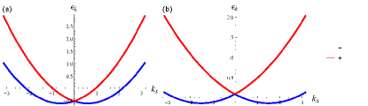
Figure 3: 2D helical bands respectively with weak spin-orbit coupling, and strong spin-orbit coupling resulting in one of the helical bands pushed above $E_{F}$.

The helicity and d-vector define two independent spin quantization axes. Suppose first that the Rashba and d-vector rotate with the same (positive) chirality around the Fermi surface; in this case the angle $\theta$ between these two axes is constant and we can write

$$\vec{d}({\bf k})=\cos\theta\hat{n}({{\bf k}})+\sin\theta\hat{\bf k}$$ (11)

When $\theta=0$, the two quantization axes align, ${\bf d}({\bf k})=\hat{n}({{\bf k}})$. In this case, the pairing and Rashba term commute, $[\hat{R}_{{\bf k}},\ \psi^{\dagger}_{{\bf k}}({\hat{\bf d}({\bf k})}\cdot\vec{\sigma})\psi_{{\bf k}}]=0$ so helicity becomes a conserved quantum number and the Bogoliubov quasi-particles acquire a definite helicity. If we introduce the projection operator onto the helical basis,

$${\cal P_{\beta}}=\frac{1}{2}\left(1+\beta\hat{n}({{\bf k}})\cdot\vec{\sigma}\right),\qquad(\beta=\pm 1)$$ (12)

then the Hamiltonian can be written

$${\cal H}_{{\bf k}} = \biggl{[}(\epsilon_{{\bf k}}+\lambda_{{\bf k}})\gamma_{3}+\Delta\gamma_{1}\biggl{]}P_{+}$$ (13)

$$+ \biggl{[}(\epsilon_{{\bf k}}-\lambda_{{\bf k}})\gamma_{3}-\Delta\gamma_{1}\biggl{]}P_{+}$$ (14)

This describes paired Fermi surfaces with “s-wave” pair condensates of opposite sign and dispersion

$$E^{\pm}({\bf k}) = \left[(\epsilon_{{\bf k}}\pm\lambda_{{\bf k}})^{2}+\Delta^{2}\right]^{1/2}.$$ (15)

More generally, we can write

$${\cal H}_{{{\bf k}}} = [\epsilon_{{\bf k}}+\lambda_{{\bf k}}\beta_{3}({\bf k})]\tau_{3}+[\Delta_{\parallel{\bf k}}\beta_{3}({\bf k})+\Delta_{\perp{\bf k}}\beta_{1}({\bf k})]\tau_{1}$$ (16)

Here $\beta_{3}({\bf k})=\hat{n}({{\bf k}})\cdot\vec{\sigma}$ and $\beta_{1}({\bf k})=\hat{\bf k}\cdot\vec{\sigma}$. For a positive chirality state $\Delta_{\parallel{\bf k}}=\Delta\cos\theta$ and $\Delta_{\perp{\bf k}}=\Delta\sin\theta$ are the pairing components parallel and perpendicular to the helicity axis $\hat{n}({{\bf k}})$, respectively. So long as $\cos\theta\neq 0$, the diagonal component of the gap preserves the $s^{\pm}$ symmetry. Thus when the the $\hat{n}({{\bf k}})$ and $\hat{d}({{\bf k}})$ rotate in the same sense, we obtain a $J=0$ $d$-wave superfluid ground state.

However, when the $\hat{d}({{\bf k}})$ vectors have a negative chirality, rotating in the opposite direction to the helicity vector $\hat{n}({{\bf k}})$ a different kind of behavior occurs. Now

$$\hat{d}({{\bf k}}) = cos(2\theta_{{\bf k}}+\phi)\hat{n}({{\bf k}})+sin(2\theta_{{\bf k}}+\phi)\hat{{\bf k}}$$ (18)

where $\theta_{{\bf k}}$ is the azimuthal angle around the Fermi surface, $\theta_{{\bf k}}=\tan^{-1}\tfrac{k_{x}}{k_{y}}$, and $\phi$ is the relative angle between $\hat{n}({{\bf k}})$ and $\hat{d}({{\bf k}})$ at $\theta_{{\bf k}}=0$. The symmetry of the superfluid state is determined by the diagonal, intra-band component of the pairing in the helical quasi-particle basis, i.e. $\Delta_{\parallel{\bf k}}$ in Eq. 13. From Eq. 18, we see that this is equal to,

$$\Delta^{J=2}_{{\bf k}} = \Delta cos(2\theta_{{\bf k}}+\phi)$$ (19)

Thus when the the $\hat{n}({{\bf k}})$ and $\hat{d}({{\bf k}})$ counter-rotate, we obtain a $J=2$ $d$-wave superfluid ground state.

The full Green’s function of the system is given by $\mathcal{G}(z)=(z-{\cal H}_{{\bf k}})^{-1}$, and the Bogoliubov spectrum is determined by the poles of $\mathcal{G}$, which gives,

$$E^{\pm}({\bf k}) = \left[\epsilon_{{\bf k}}^{2}+\lambda_{{\bf k}}^{2}+\Delta^{2}\right.$$ (21)

$$\pm 2\left.\left[\lambda_{{\bf k}}^{2}\epsilon_{{\bf k}}^{2}+\lambda_{{\bf k}}^{2}\Delta^{2}|\hat{n}_{{\bf k}}\times\hat{d}_{{\bf k}}|^{2}\right]\right]^{1/2}$$

The Bogoliubov spectrum can also be written as,

$$E^{\pm}({\bf k})=\left[A_{{\bf k}}\pm\sqrt{A_{{\bf k}}^{2}-\gamma_{{\bf k}}^{2}}\right]^{1/2}$$ (22)

where $A_{{\bf k}}=\epsilon_{{\bf k}}^{2}+\lambda_{{\bf k}}^{2}+\Delta^{2}$ and

$$\gamma_{{\bf k}}^{2}=(\epsilon_{{\bf k}}^{2}-\lambda_{{\bf k}}^{2}+\Delta^{2})^{2}+4(\lambda_{{\bf k}}\Delta\,\hat{n}({{\bf k}})\cdot\hat{d}({{\bf k}}))^{2}$$ (23)

Since $(E^{+}E^{-})^{2}=\gamma_{{\bf k}}^{2}$, it follows that when $\hat{n}({{\bf k}})\cdot\hat{d}({{\bf k}})\neq 0$, $E^{+}E^{-}$ is positive definite, and the gap is finite. If $\hat{n}({{\bf k}})$ and $\hat{d}({{\bf k}})$ rotate in the same sense, the gap is finite everywhere and and maximized when $\hat{n}({{\bf k}})$ are $\hat{d}({{\bf k}})$ are parallel, i.e $\hat{n}({{\bf k}})\times\hat{d}({{\bf k}})=0$. In a mean-field theory, the system selects this minimum energy state dynamically, generating an internal Josephson coupling that couples the two pairing channels such that the $\hat{d}({{\bf k}})$ vector lies parallel to the spin-orbit field $\hat{n}({{\bf k}})$. By contrast, when $\hat{n}({{\bf k}})$ and $\hat{d}({{\bf k}})$ counter rotate, $\gamma_{{\bf k}}^{2}=0$ along the nodes of $cos(2\theta_{{\bf k}}+\phi)$, which is the rotation of a $d_{xy}$ state through angle $-\phi$. The gap nodes occur at locations where $\gamma_{{\bf k}}=0$, i.e at the intersection of the nodal lines of $cos(2\theta_{{\bf k}}+\phi)$ and the surfaces defined by $\epsilon_{{\bf k}}^{2}-\lambda^{2}+\Delta^{2}=0$.

III Topological $s^{\pm}$ & $d$-wave State with Gapless Edge States

The topology of ³He-B is protected by time-reversal symmetry ($\mathcal{T}$) with an invariant given by Eq. 9, and there are corresponding time-reversal protected gapless chiral edge states. Since the spin-orbit coupling $\hat{n}({{\bf k}})\cdot\vec{\sigma}$ is time-reversal invariant, it will not mix the left and right-moving Majorana fermions. Furthermore, the system remains fully gapped it is adiabatically evolved from the ³He-B state into the $s^{\pm}$ state by switching on the spin-orbit coupling. Hence, we expect the low angular momentum $s^{\pm}$ state to remain topological and exhibit gapless chiral edge states.

For completeness, we calculate the edge states at the domain wall between two bulk ³He-R of opposite chirality, satisfying the boundary conditions $\Delta_{2}(x=-\infty)=-\Delta_{2}$ and $\Delta_{2}(x=\infty)=+\Delta_{2}$, using the method described by Volovik (2009a). This calculation is equivalent to the calculation of reflection at a boundary along the plane $x=0$ of the superfluid, since the Rasbha and pairing fields of a fermion reflecting at normal incidence off the boundary electron, reverse. The topological invariant $n$ (Eq. 9) changes sign from $+1$ to $-1$ across the domain, when $\Delta(x)$ changes sign. Similarly, $\lambda(x)$ changes sign so that the system remains in a $J=0$ $s^{\pm}$ state on both sides of the domain. For small $k_{x}^{2}\ll k_{F}^{2}$, we can calculate the edge states perturbatively. Letting $k_{x}=k_{F}+i\partial_{x}$, we obtain the Hamiltonian,

$$H = H^{(0)}+H^{{}^{\prime}}$$ (24)

$$H^{(0)} = iv_{F}\partial_{x}\gamma_{3}+\lambda(x)\sigma_{2}\gamma_{3}+\Delta_{2}(x)\sigma_{2}\gamma_{1}$$ (25)

$$H^{{}^{\prime}} = \frac{\Delta_{1}}{k_{F}}k_{y}\sigma_{1}\gamma_{1}+\frac{\lambda}{k_{F}}k_{y}\sigma_{1}\gamma_{3}$$ (26)

where $v_{F}=\tfrac{k_{F}}{m}$. There are two zero-energy solutions, $\psi_{+}$ and $\psi_{-}$ corresponding to $\sigma_{2}=\pm 1$ respectively.

$$\psi_{\pm}(x) = {\mathrm{e}xp}\left[{-\frac{1}{v_{F}}\int_{0}^{x}dx^{\prime}\left(\Delta_{2}(x^{\prime})-i\lambda(x^{\prime})\sigma_{2}\right)}\right]\xi_{\pm},$$ (27)

$$\xi_{\pm} = \begin{pmatrix}1\\ \pm i\end{pmatrix}_{\gamma}\!\!\!\begin{pmatrix}1\\ \pm i\end{pmatrix}_{\sigma}.$$ (28)

It is straightforward to show that the zero-energy modes satisfy the following Hamiltonian along the edge, and disperse linearly.

$$\begin{bmatrix}H^{{}^{\prime}}_{++}&H^{{}^{\prime}}_{+-}\\ H^{{}^{\prime}}_{-+}&H^{{}^{\prime}}_{--}\\ \end{bmatrix}=\begin{bmatrix}0&(v-i\delta)k_{y}\\ (v+i\delta)k_{y}&0\\ \end{bmatrix}$$ (29)

where,

$$v = \left(\int_{-\infty}^{\infty}dx\frac{\Delta_{1}(x)}{k_{F}}exp[-\frac{2}{v_{F}}\int_{0}^{x}dx^{\prime}\Delta_{2}(x^{\prime})]\right)$$ (31)

$$\times\left(\int_{-\infty}^{\infty}exp[-\frac{2}{v_{F}}\int_{0}^{x}dx^{\prime}\Delta_{2}(x^{\prime})]\right)^{-1}$$

$$\delta = \left(\int_{-\infty}^{\infty}dy\frac{\lambda_{1}(x)}{k_{F}}exp[-\frac{2}{v_{F}}\int_{0}^{x}dx^{\prime}\Delta_{2}(x^{\prime})]\right)$$ (34)

$$\times\left(\int_{-\infty}^{\infty}exp[-\frac{2}{v_{F}}\int_{0}^{x}dx^{\prime}\Delta_{2}(x^{\prime})]\right)^{-1}$$

Solving the edge Hamiltonian, Eq. 24, gives the following two fermionic zero modes,

$$H^{{}^{\prime}}\psi_{1,2} = \pm\;ck_{y}\psi_{1,2}$$ (35)

$$\psi_{1,2} = \psi_{+}\pm\psi_{1}$$ (36)

$$c = \sqrt{v^{2}+\delta^{2}}$$ (37)

where $\psi_{1,2}$ are two linearly dispersing Majorana fermions, similar to the Majorana edge modes found in isotropic ³He-B, with a renormalization of the velocity by the spin-orbit coupling.

As explained in Sec. II, the $d$-wave state corresponds to counter-rotation of $\hat{d}_{{\bf k}}$ with respect to $\hat{n}_{{\bf k}}$, and in particular, choosing $\hat{d}_{{\bf k}}\cdot\vec{\sigma}=\hat{k}_{y}\sigma_{x}+\hat{k}_{x}\sigma_{y}$ gives a $d_{xy}$ state. Hence, an identical calculation to that carried out above, with $\Delta_{1}\rightarrow-\Delta_{1}$ shows that the $d$-wave state is also topological with gapless Majorana edges states. This is in agreement with the results of Schnyder et. al. Schnyder et al. (2012).

IV Effects of Hard-Core/Coulomb Repulsion: Topological Phase Transition Into $d$-wave State

The hard-core fermionic repulsion in ³He requires that the on-site pair amplitude is zero, $\langle\psi_{\uparrow}(\vec{x})\psi_{\downarrow}(\vec{x})\rangle=0$, and the ³He-B phase satisfies this constraint by triplet pairing in the $p$-wave channel. However, spin-orbit coupling, which allows mixing of spin and angular momentum, causes scattering of $p_{x/y}$-wave triplet pairs into $s$-wave spin-singlet Cooper pairs, and this can lead to a finite on-site $s$-wave pair amplitude.

The $s^{\pm}$ state manages to satisfy the hard-core constraint, even though there is a finite $s$-wave pair susceptibility in each $p$-wave channel, because of phase cancellation between the bands with opposite helicities. The phase cancellation mechanism is clear from the Green’s function in the helical basis, which may be calculated from Eq. 13,

$${\cal{G}}(z,{\bf k}) = \frac{1}{z-\cal{H}_{{\bf k}}}$$ (38)

$$= \sum_{\pm}\frac{z+(\epsilon_{{\bf k}}\pm\lambda_{{\bf k}})\gamma_{3}\pm\Delta\gamma_{1}}{z^{2}-E^{\pm}({\bf k})^{2}}\biggl{(}\frac{1\pm\hat{n}({{\bf k}})\cdot\vec{\sigma}}{2}\biggr{)}$$ (39)

The $\pm\Delta\gamma_{1}$ component of the Gork’ov propagator describes s-wave pairing on the two helicity split Fermi surfaces. The net $s$-wave amplitude $\langle c^{\dagger}_{\uparrow}c^{\dagger}_{\downarrow}\rangle$ is then given by,

$$\langle c^{\dagger}_{\uparrow}c^{\dagger}_{\downarrow}\rangle = \frac{T}{2}\sum_{{\bf k},n}Tr[{\cal G}(i\omega_{n},{\bf k})\frac{\gamma_{1}}{2}]$$ (41)

$$= \frac{T}{2}\sum_{{\bf k},i\omega_{n},\beta=\pm}\beta\frac{\Delta}{(i\omega_{n})^{2}-E^{\beta}({\bf k})^{2}}$$ (42)

$$= \sum_{{\bf k},\beta=\pm}\beta\tanh\left(\frac{E^{\beta}({\bf k})}{2T}\right)\frac{\Delta}{4E^{\beta}_{{\bf k}}}.$$ (43)

We can interpret the two components in Eq. 41 as the pair contributions from the two helicity polarized bands, given by

$$\langle c^{\dagger}_{{\uparrow}}c^{\dagger}_{\downarrow}\rangle_{\pm}=\pm\sum_{{\bf k}}\tanh\left(\frac{E^{\pm}({\bf k})}{2T}\right)\frac{\Delta}{4E^{\pm}_{{\bf k}}}.$$ (44)

confirming that each band contributes an s-wave pairing amplitude of opposite signs. In the limit of weak spin-orbit coupling, when $E^{+}({\bf k})\approx E^{-}({\bf k})$, there is almost complete phase cancellation between the two helical bands, and $\langle c^{\dagger}_{\uparrow}c^{\dagger}_{\downarrow}\rangle\approx 0$. However, this mechanism fails when the spin-orbit coupling becomes comparable to the kinetic energy, such that one of the bands is shifted away from the Fermi surface; a phase transition to a $d$-wave state will then occur.

We now include a Hubbard interaction to account for the hard-core repulsion, and then carry out a Hubbard-Stratonovich decomposition into an $s$-wave term

$$H^{(U)} = U\sum_{i}n_{i\uparrow}n_{i\downarrow}\equiv U\sum_{i}(c^{\dagger}_{i{\uparrow}}c^{\dagger}_{i{\downarrow}})(c_{i{\downarrow}}c_{i{\uparrow}})$$ (45)

$$\longrightarrow \sum_{i}\Delta_{s}\,c^{\dagger}_{\uparrow i}c^{\dagger}_{\downarrow i}+H.c.-\frac{|\Delta_{s}|^{2}}{U}$$ (46)

At the saddle point of the mean-field free energy where $\partial F/\partial\Delta_{s}=0$, the pair density is given by $\langle c^{\dagger}_{i{\uparrow}}c^{\dagger}_{i{\downarrow}}\rangle=\bar{\Delta}_{s}/U$, and in the large $U$ limit, this becomes the constraint

$$\hskip 71.13188pt\langle c_{\uparrow}(\vec{x})c_{\downarrow}(\vec{x})\rangle=0\hskip 34.14322pt(U\rightarrow\infty)$$ (47)

After including the $s$-wave pairing, the Hamiltonian is now written as,

$$\cal{H}_{{\bf k}} = \sum_{\beta=\pm}\biggl{[}(\epsilon_{{\bf k}}+\beta\lambda_{{\bf k}})\gamma_{3}+(\beta\Delta+\Delta_{s})\gamma_{1}\biggl{]}P_{\beta}$$ (48)

and the Bogoliubov spectrum is then given by,

$$E^{\beta}({\bf k}) = \left[(\epsilon_{{\bf k}}+\beta\lambda_{{\bf k}})^{2}+(\Delta+\beta\Delta_{s})^{2}\right]^{1/2}$$ (49)

It is now straightforward to calculate the free energy and the $s$-wave amplitude.

$$F = N_{s}\left[\frac{\Delta_{1}^{2}}{g_{1}}+\frac{\Delta_{2}^{2}}{g_{2}}\right]$$

$$-2T\sum_{{\bf k},\alpha}\ln\left[2\cosh\left(\frac{E^{\alpha}_{{\bf k}}}{2T}\right)\right]$$

The stationarity condition becomes

$$\frac{\partial F}{\partial\Delta_{s}}=\langle c_{\uparrow}^{{}^{\dagger}}c_{\downarrow}^{{}^{\dagger}}\rangle=\langle c^{{}^{\dagger}}_{\uparrow}c^{{}^{\dagger}}_{\downarrow}\rangle_{+}+\langle c^{{}^{\dagger}}_{\uparrow}c^{{}^{\dagger}}_{\downarrow}\rangle_{-}=0$$ (51)

where by direct differentiation, we recover the result of Eq. 41,

$$\langle c^{\dagger}_{{\uparrow}}c^{\dagger}_{\downarrow}\rangle_{\pm}=\pm\sum_{{\bf k}}\tanh\left(\frac{E^{\pm}({\bf k})}{2T}\right)\frac{\Delta}{4E^{\pm}_{{\bf k}}}.$$ (52)

We now use a simplified momentum-independent spin-orbit coupling $\lambda_{{\bf k}}=\lambda$ to demonstrate the key physics of phase cancellation in 2D. In this simplified model, the helical bands are split apart by $\lambda$, and the density of state of both bands remain constant. The integral in Eq. 52 gives the standard BCS result,

$$\langle c^{\dagger}_{{\uparrow}}c^{\dagger}_{\downarrow}\rangle_{\pm}=\pm\frac{N(0)\Delta}{2}\ln\frac{\omega_{sf}}{\Delta}$$ (53)

where $\omega_{sf}$ is the characteristic upper cutoff of the p-wave pairing attraction (spin-fluctuation) energy scale and $N(0)$ is the density of states. In this simple case, $\langle c^{{}^{\dagger}}_{\uparrow}c^{{}^{\dagger}}_{\downarrow}\rangle_{+}$ and $\langle c^{{}^{\dagger}}_{\uparrow}c^{{}^{\dagger}}_{\downarrow}\rangle_{-}$ exactly cancel. Thus, in the case of weak to moderate spin-orbit coupling, when both helical bands still cross $E_{F}$, there is zero net $s$-wave Cooper pair amplitude due to phase cancellation of $s^{\pm}$ state on both bands.

However, when the spin-orbit coupling becomes comparable to the kinetic energy and shifts one of the bands away from $E_{F}$, there will now be a net $s$-wave pair scattering amplitude. In the quasi-particle basis, this means that the $s^{\pm}$ state is transformed into an $s^{++}$ state as there is only one helical band with an $s^{++}$ pairing crossing $E_{F}$.

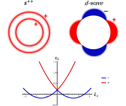
Figure 4: Strong spin-orbit coupling scenario: in the absence of Coulomb repulsion, the $s^{pm}$ state is transformed into an $s^{++}$ state on the remaining helical band. In the presence of Coulomb repulsion, the on-site $s$-wave pair amplitude is disfavored, and the system will instead favor a phase transition into a $d$-wave state to minimize the hard-core/Coulomb repulsion. (Technically, the superfluid pairing on the lower helical band has a phase proportional to $\beta=-$, but we follow convention in labelling it as an $s^{++}$ pairing, which is equivalent up to a gauge transformation.)

This fully gapped $s^{++}$ state is energetically favored in the absence of hard-core/Coulomb repulsion. However, in the presence of a hard-core/Coulomb repulsion, the finite on-site $s$-wave pair amplitude is strongly disfavored, and the system will instead undergo a topological phase transition into a $d$-wave state, as illustrated in Fig. 2. The positions of the nodes will be determined by the relative orientation ($\phi$) of the $\hat{d}_{{\bf k}}$-vector with respect to the spin-orbit $\hat{n}_{{\bf k}}$-vector, and this corresponds to an additional $U(1)$ gauge degree of freedom. For $\phi=0$, we will get a $d_{x^{2}-y^{2}}$ state, while $\phi=\tfrac{\pi}{2}$ will correspond to a $d_{xy}$ state. The $d$-wave state will not be topological, as the gapless fermionic excitations along the nodes in the $d$-wave superfluid state will couple to the gapless Majorana edge states in general.

For a realistic momentum-dependent spin-orbit coupling, $\lambda_{{\bf k}}=\lambda|\vec{k}|$, these results remain qualitatively correct, with corrections due to renormalization of $N(0)$ by the spin-orbit coupling. In this case, the phase cancellation will not be exact, and the phase transition will occur before the upper helical band is completely lifted above $E_{F}$.

V Discussion

Using a Rashba coupled model of two dimensional superfluid He-3B, “³He-R”, we have demonstrated that in the presence of a strong Rashba coupling, a single underlying microscopic pairing mechanism can give rise to two superfluid/superconducting ground states of different symmetry : a low “spin” fully gapped topological $s^{\pm}$ state, and a high “spin” gapless $d$-wave state. This is because the spin and rotational symmetries of a system are coupled by spin-orbit coupling, i.e. $SU(2)_{S}\otimes SO(3)_{L}\rightarrow SO(3)_{J}$.

In contrast to previous works Frigeri et al. (2004); Sato and Fujimoto (2009); Tanaka et al. (2010); Schnyder et al. (2012) on non-centrosymmetric superconductors, where they assumed that the $\hat{n}_{{\bf k}}$ and $\hat{d}_{{\bf k}}$ vectors are parallel due to strong spin-orbit coupling, we take into account the additional $U(1)$ rotational degree of freedom, which gives rise to a low “spin” to high “spin” transition. We show that the strong Coulomb repulsion breaks the alignment of $\hat{n}_{{\bf k}}$ and $\hat{d}_{{\bf k}}$, and the mixing of $s$ and $d$-wave spin-singlet, with $p$-wave spin-triplet pairing naturally arises from the in-phase and counter-phase rotation of $\hat{n}_{{\bf k}}$ and $\hat{d}_{{\bf k}}$ respectively. Whereas, the $d$-wave state obtained in previous results are generated by an $f$-wave triplet pair rotating in-phase with $\hat{n}_{{\bf k}}$, i.e. a $J=3-1=2$ state.

Since the spin-orbit coupling is time-reversal invariant, the topological nature of the fully gapped ³He-B state is protected for weak spin-orbit coupling. In this limit, the ground state of the system is a fully gapped topological $s^{\pm}$ state, and we show using an explicit calculation that the gapless Majorana edge states survive, in agreement with Sato and FujimotoSato and Fujimoto (2009).

However, on-site Coulomb or hard-core repulsion will drive the system towards a higher angular momentum $d$-wave state when the spin-orbit coupling is sufficiently large to lift one of the helical bands above the Fermi surface. The phase cancellation mechanism that minimizes the on-site $s$-wave pair amplitude for the $s^{\pm}$ state is then no longer effective, and the system will undergo a topological phase transition to a topological $d$-wave stateSchnyder et al. (2012).

Such a topological phase transition may exist at the boundary between the crust and quantum interior of neutron stars where the transition from an $s^{\pm}$ to a $d$-wave superfluid state would be driven by the rise in short-range repulsion with increasing density David Pines (1985). This would mean that Majorana fermions already exist in one of the largest superfluid systems known in nature.

This work also raises the intriguing possibility that the $s^{\pm}$ superconducting state believed to exist in iron-based superconductors could have a higher angular momentum microscopic pairing mechanism, which is hidden behind a non-trivial helical quasi-particle structure. In these systems, the $d_{xz}$ and $d_{yz}$ atomic orbitals form an iso-spin $(\vec{\alpha})$ representation, which plays a similar role to spin here, $\vec{\sigma}\leftrightarrow\vec{\alpha}$. There is a large orbital Rashba coupling in the Fe systems, $\lambda_{{\bf k}}\sim E_{F}$, and a microscopic $d$-wave orbital triplet pairingOng and Coleman (2013) will give rise to a $J=L+\alpha=0$ $s^{\pm}$ state or a $J=4$ $g$-wave state. This possibility will be discussed in future work.

We thank Onur Erten for helpful discussions. We also thank Andreas Schnyder and Philip Brydon for pointing out the topological nature of the $d$-wave state, and for very helpful discussions. This work is supported by DOE grant DE-FG02-99ER45790.

References

- Volovik (2003) G. E. Volovik, The Universe in a Helium Droplet (Clarendon Press, UK, 2003).
- Schnyder et al. (2008) A. P. Schnyder, S. Ryu, A. Furusaki, and A. W. W. Ludwig, Phys. Rev. B 78, 195125 (2008).
- Ryu et al. (2010) S. Ryu, A. P. Schnyder, A. Furusaki, and A. W. W. Ludwig, New Journal of Physics 12, 065010 (2010).
- Qi and Zhang (2011) X.-L. Qi and S.-C. Zhang, Rev. Mod. Phys. 83 (2011), 10.1103/RevModPhys.83.1057.
- Fu and Kane (2008) L. Fu and C. L. Kane, Phys. Rev. Lett. 100, 096407 (2008).
- Sau et al. (2010) J. D. Sau, R. M. Lutchyn, S. Tewari, and S. Das Sarma, Phys. Rev. Lett. 104, 040502 (2010).
- Oreg et al. (2010) Y. Oreg, G. Refael, and F. von Oppen, Phys. Rev. Lett. 105, 177002 (2010).
- Rice and Sigrist (1995) T. M. Rice and M. Sigrist, Journal of Physics: Condensed Matter 7, L643 (1995).
- Ishida et al. (1998) K. Ishida, H. Mukuda, Y. Kitaoka, K. Asayama, Z. Q. Mao, Y. Mori, and Y. Maeno, Nature 396, 658 (1998).
- Luke et al. (1998) G. M. Luke, Y. Fudamoto, K. M. Kojima, M. I. Larkin, J. Merrin, B. Nachumi, Y. J. Uemura, Y. Maeno, Z. Q. Mao, Y. Mori, H. Nakamura, and M. Sigrist, Nature 394, 558 (1998).
- Mackenzie and Maeno (2003) A. P. Mackenzie and Y. Maeno, Rev. Mod. Phys. 75, 657 (2003).
- Vollhardt and Wölfle (2013) D. Vollhardt and P. Wölfle, The Superfluid Phases of Helium 3 (Dover Publications, UK, 2013).
- Balian and Werthamer (1963) R. Balian and N. R. Werthamer, Phys. Rev. 131, 1553 (1963).
- Osheroff (1997) D. D. Osheroff, Rev. Mod. Phys. 69, 667 (1997).
- Leggett (1975) A. J. Leggett, Rev. Mod. Phys. 47, 331 (1975).
- Wheatley (1975) J. C. Wheatley, Rev. Mod. Phys. 47, 415 (1975).
- Anderson and Morel (1961) P. W. Anderson and P. Morel, Phys. Rev. 123, 1911 (1961).
- Volovik (2009a) G. Volovik, JETP Letters 90, 398 (2009a).
- Volovik (2009b) G. Volovik, JETP Letters 90, 587 (2009b).
- Qi et al. (2009) X.-L. Qi, T. L. Hughes, S. Raghu, and S.-C. Zhang, Phys. Rev. Lett. 102, 187001 (2009).
- Wu and Sauls (2013) H. Wu and J. A. Sauls, “Majorana excitations: Spin- and mass currents on the surface of the topological superfluid 3he-b,” (2013), arXiv:1308.4436 [”cond-mat”] .
- Frigeri et al. (2004) P. A. Frigeri, D. F. Agterberg, A. Koga, and M. Sigrist, Phys. Rev. Lett. 92, 097001 (2004).
- Sato and Fujimoto (2009) M. Sato and S. Fujimoto, Phys. Rev. B 79, 094504 (2009).
- Tanaka et al. (2010) Y. Tanaka, Y. Mizuno, T. Yokoyama, K. Yada, and M. Sato, Phys. Rev. Lett. 105, 097002 (2010).
- David Pines (1985) M. A. A. David Pines, Nature , 27 32 (1985).
- Hoffberg et al. (1970) M. Hoffberg, A. E. Glassgold, R. W. Richardson, and M. Ruderman, Phys. Rev. Lett. 24, 775 (1970).
- Y.-J. Lin (2011) I. B. S. Y.-J. Lin, K. Jimenez-Garcia, Nature , 83 86 (2011).
- Ong and Coleman (2013) T. T. Ong and P. Coleman, Phys. Rev. Lett. 111, 217003 (2013).
- Schnyder et al. (2012) A. P. Schnyder, P. M. R. Brydon, and C. Timm, Phys. Rev. B 85, 024522 (2012).