Lévy flights in inhomogeneous environments and $1/f$ noise

Abstract

Complex dynamical systems which are governed by anomalous diffusion often can be described by Langevin equations driven by Lévy stable noise. In this article we generalize nonlinear stochastic differential equations driven by Gaussian noise and generating signals with $1/f$ power spectral density by replacing the Gaussian noise with a more general Lévy stable noise. The equations with the Gaussian noise arise as a special case when the index of stability $\alpha=2$. We expect that this generalization may be useful for describing $1/f$ fluctuations in the systems subjected to Lévy stable noise.

I Introduction

The Lévy $\alpha$-stable distributions, characterized by the index of stability $0<\alpha\leqslant 2$, constitute the most general class of stable processes. The Gaussian distribution is their special case, corresponding to $\alpha=2$. If $\alpha<2$, the Lévy stable distributions have power-law tails $\sim 1/x^{1+\alpha}$. There are many systems exhibiting Lévy $\alpha$-stable distributions: distribution function of turbulent magnetized plasma emitters Marandet et al. (2003) and step-size distribution of photons in hot vapors of atoms Mercadier et al. (2009) have Lévy tails; theoretical models suggest that velocity distribution of particles in fractal turbulence is Lévy stable distribution Takayasu (1984) or at least has Lévy tails Min et al. (1996). If system behavior depends only on large noise fluctuations, such noise intensity distributions can by approximated by Lévy stable distribution, leading to Lévy flights. Lévy flight is a generalization of the Brownian motion which describes the motion of small macroscopic particles in a liquid or a gas experiencing unbalanced bombardments due to surrounding atoms. The Brownian motion mimics the influence of the “bath” of surrounding molecules in terms of time-dependent stochastic force which is commonly assumed to be white Gaussian noise. That postulate is compatible with the assumption of a short correlation time of fluctuations, much shorter than the time scale of the macroscopic motion, and the assumption of weak interactions with the bath. In contrast, the Lévy motions describe results of strong collisions between the particle and the surrounding environment. Lévy flights can be found in many physical systems: as an example we can point out anomalous diffusion of Na adatoms on solid Cu surface Guantes et al. (2001), anomalous diffusion of a gold nanocrystal, adsorbed on the basal plane of graphite Luedtke and Landman (1999) and anomalous diffusion in optical lattices Marksteiner et al. (1996). Lévy flights can be modeled by fractional Fokker-Planck equations Fogedby (1994a) or Langevin equations with additive Lévy stable noise.

Nonlinear stochastic differential equations (SDEs) with additive Lévy stable noise have been explored quite extensive for past 15 years Jespersen et al. (1999); Chechkin et al. (2002); Eliazar and Klafter (2003); Denisov et al. (2008). Such stochastic differential equations lead to fractional Fokker-Planck equations with constant diffusion coefficient. Models with multiplicative Lévy stable noise have been used for modeling inhomogeneous media Srokowski (2009a), ecological population density with fluctuating volume of resources Dubkov (2012). The relation between Langevin equation with multiplicative Lévy stable noise and fractional Fokker-Planck equation has been introduced in Ref. Schertzer et al. (2001), where Langevin equation is interpreted in Itô sense Srokowski (2009b). The relation between these two equation are not known in Stratonovich interpretation. Fractional Fokker-Planck equation models have been applied to model enzyme diffusion on polymer chain Lomholt et al. (2005) and some cases of anomalous diffusion Srokowski and Kaminska (2006). However, application of Lévy stable noise driven SDEs can be problematic. We can always write Fokker-Planck equation corresponding to Langevin equation driven by Gaussian noise and vice versa, but such statement is not always true for Langevin equation with Lévy stable noise. For example, particle (enzyme) dispersion on rapidly folding random heteropolymer can be described by space fractional Fokker-Planck equation Brockmann and Geisel (2003a), but for such equation counterpart Langevin equation has not been found Brockmann and Sokolov (2002) and might not even exits Brockmann and Geisel (2003b).

One of the characteristics of the signal is the power spectral density (PSD). Signals having the PSD at low frequencies $f$ of the form $S(f)\sim 1/f^{\beta}$ with $\beta$ close to $1$ are commonly referred to as “$1/f$ noise”, “$1/f$ fluctuations”, or “flicker noise”. Power-law distributions of spectra of signals with $0.5<\beta<1.5$, as well as scaling behavior are ubiquitous in physics and in many other fields Ward and Greenwood (2007); *Weissman1988; *Barabasi1999; *Gisiger2001; *Wagenmakers2004; *Szabo2007; *Castellano2009. Despite the numerous models and theories proposed since its discovery more than 80 years ago Johnson (1925); *Schottky1926, the subject of $1/f$ noise remains still open for new discoveries. Most models and theories of $1/f$ noise are not universal because of the assumptions specific to the problem under consideration. A short categorization of the theories and models of $1/f$ noise is presented in the introduction of the paper Kaulakys and Alaburda (2009), see also recent review by Balandin Balandin (2013). Mostly $1/f$ noise is considered as Gaussian process Kogan (2008); Li and Zhao (2012), but sometimes the signal exhibiting $1/f$ fluctuations are non-Gaussian Orlyanchik et al. (2008); Melkonyan (2010).

Often $1/f$ noise is modeled as the superposition of Lorentzian spectra with a wide range distribution of relaxation times McWhorter (1957). An influential class of the models of $1/f$ noise involves self-organized criticality (SOC) Bak et al. (1987); *Jensen1989; *Kertesz1990. One more way of obtaining $1/f$ noise from a signal consisting of pulses has been presented in Kaulakys and Meškauskas (1998); *Kaulakys1999; *Kaulakys2000-2; *Kaulakys2005: it has been shown that the intrinsic origin of $1/f$ noise may be a Brownian motion of the interevent time of the signal pulses. The nonlinear SDEs generating signals with $1/f$ noise were obtained in Refs. Kaulakys and Ruseckas (2004); Kaulakys et al. (2006) (see also papers Kaulakys and Alaburda (2009); Ruseckas and Kaulakys (2010); *Ruseckas2011), starting from the point process model of $1/f$ noise. A special case of this SDE has been obtained using Kirman’s agent model Ruseckas et al. (2011). Such nonlinear SDEs were used to describe signals in socio-economical systems Gontis et al. (2010); Mathiesen et al. (2013).

The purpose of this paper is to generalize nonlinear SDEs driven by Gaussian noise and generating signals with $1/f$ PSD by replacing the Gaussian noise with a more general Lévy stable noise. The previously proposed SDEs then arise as a special case when $\alpha=2$. We can expect that this generalization may be useful for describing $1/f$ fluctuations in the systems subjected to Lévy stable noise.

The paper is organized as follows: In Section II we search for the nonlinear SDE with Lévy stable noise yielding power law steady state probability density function (PDF) of the generated signal. In Section III we estimate when the signal generated by such an SDE has $1/f$ PSD in a wide region of frequencies. In Section IV we numerically solve obtained equations and compare the PDF and PSD of the signal with analytical estimations. Section V summarizes our findings.

II Stochastic differential equation with Lévy stable noise generating signals with power law distribution

In this Section we search for nonlinear SDEs with Lévy stable noise yielding power law steady state PDF of the generated signal. We consider the Langevin equation of the form Fogedby (1994a, b, 1998)

$$\frac{dx}{dt}=a(x)+b(x)\xi(t)\,,$$ (1)

where $a(x)$ and $b(x)$ are given functions describing the deterministic drift term and the amplitude of the noise, respectively. The stochastic force $\xi(t)$ is uncorrelated, $\langle\xi(t)\xi(t^{\prime})\rangle=\delta(t-t^{\prime})$ and is characterized by Lévy $\alpha$-stable distribution. In this paper we will restrict our investigation only to symmetric stable distributions, thus the characteristic function of $\xi(t)$ is

$$\langle\exp(ik\xi)\rangle=\exp(-\sigma^{\alpha}|k|^{\alpha})\,.$$ (2)

Here $\alpha$ is the index of stability and $\sigma$ is the scale parameter. We interpret Eq. (1) in Itô sense. In mathematically more formal way Eq. (1) can be written in the form

$$dx=a(x)+b(x)dL_{t}^{\alpha}\,,$$ (3)

where $dL_{t}^{\alpha}$ stands for the increments of Lévy $\alpha$-stable motion $L_{t}^{\alpha}$ Janicki and Weron (1994); Weron et al. (2005). For calculating of the steady state PDF of the signal $x$ we will use the fractional Fokker-Planck equation instead of stochastic differential equation (1). The fractional Fokker-Planck equation corresponding to Itô solution of Eq. (1) is Ditlevsen (1999); Schertzer et al. (2001)

$$\frac{\partial}{\partial t}P(x,t)=-\frac{\partial}{\partial x}a(x)P(x,t)+\sigma^{\alpha}\frac{\partial^{\alpha}}{\partial|x|^{\alpha}}b(x)^{\alpha}P(x,t)\,.$$ (4)

Here $\partial^{\alpha}/\partial|x|^{\alpha}$ is the Riesz-Weyl fractional derivative. The Riesz-Weyl fractional derivative of the function $f(x)$ is defined by its Fourier transform Samko et al. (1993),

$$\mathcal{F}\left[\frac{\partial^{\alpha}}{\partial|x|^{\alpha}}f(x)\right]=-|k|^{\alpha}\tilde{f}(k)\,.$$ (5)

One can get the following expression for the Riesz-Weyl derivative :

$$\frac{\partial^{\alpha}}{\partial|x|^{\alpha}}f(x)=-\frac{1}{2\cos\left(\frac{\pi\alpha}{2}\right)}\{D_{+}^{-\alpha}f(x)+D_{-}^{-\alpha}f(x)\}\,,$$ (6)

where $D_{+}^{-\alpha}$ and $D_{-}^{-\alpha}$ are the left and right Riemann-Liouville derivatives Samko et al. (1993):

$$D_{\pm}^{-\alpha}=(\pm 1)^{m}\frac{d^{m}}{dx^{m}}D_{\pm}^{m-\alpha}\,,\qquad m-1<\alpha<m\,.$$ (7)

Here $m$ is an integer and

$$D_{+}^{\alpha}f(x) = \frac{1}{\Gamma(\alpha)}\int_{-\infty}^{x}(x-z)^{\alpha-1}f(z)\,dz\,,$$ (8)

$$D_{-}^{\alpha}f(x) = \frac{1}{\Gamma(\alpha)}\int_{x}^{+\infty}(z-x)^{\alpha-1}f(z)\,dz\,.$$ (9)

When $\alpha=1$ then the definition of the Riesz-Weyl derivative is

$$\frac{d}{d|x|}f(x)=-\frac{d}{dx}\frac{1}{\pi}\int_{-\infty}^{+\infty}\frac{f(z)}{x-z}\,dz\,.$$ (10)

Eq. (4) leads to the following equation for the steady state PDF:

$$\sigma^{\alpha}\frac{\partial^{\alpha}}{\partial|x|^{\alpha}}b(x)^{\alpha}P_{0}(x)-\frac{\partial}{\partial x}a(x)P_{0}(x)=0\,.$$ (11)

Equation (11) can be written as $-dJ(x)/dx=0$, where $J(x)$ is the probability current. Reflective boundaries lead to the boundary condition $J(x)=0$.

II.1 Equation with only positive values of $x$

We will search for the stochastic differential equation (1) generating signals with power law steady state PDF,

$$P_{0}(x)\sim x^{-\lambda}\,.$$ (12)

Since power law PDF cannot be normalized when $x$ can vary from zero to infinity, we will assume that the power law holds only in some wide region of $x$, $x_{\mathrm{min}}\ll x\ll x_{\mathrm{max}}$. One can expect that power law PDF can be obtained when the coefficients $a(x)$ and $b(x)$ in Eq. (1) themselves are of the power law form. Thus we will consider $b(x)=x^{\eta}$ and $a(x)=\sigma^{\alpha}\gamma x^{\mu}$. Here $\eta$ is the exponent of the multiplicative noise, $\mu$ and $\gamma$ are to be determined. With such a choice of $b(x)$ and power law form of $P_{0}(x)$ from Eq. (4) it follows that we need to calculate fractional derivative of the the power law function.

Let us consider the function

$$f(x)=\begin{cases}x^{\rho}\,,&x_{\mathrm{min}}<x<x_{\mathrm{max}}\,,\\ 0&\mbox{otherwise .}\end{cases}$$ (13)

Using Eq. (6) we obtain the following approximate expressions for the fractional derivative of the function (13) when $x_{\mathrm{min}}\ll x\ll x_{\mathrm{max}}$:

$$\frac{d^{\alpha}}{d|x|^{\alpha}}f(x)\approx\begin{cases}\frac{\sin\left(\pi\left(\frac{\alpha}{2}-\rho\right)\right)}{\sin(\pi(\rho-\alpha))}\frac{\Gamma(1+\rho)}{\Gamma(1+\rho-\alpha)}x^{\rho-\alpha}\,,&-1<\rho<\alpha\,,\\ \frac{x_{\mathrm{min}}^{1+\rho}}{2\cos\left(\frac{\pi}{2}\alpha\right)(1+\rho)\Gamma(-\alpha)}x^{-1-\alpha}\,,&\rho<-1\\ \frac{x_{\mathrm{max}}^{\rho-\alpha}}{2\cos\left(\frac{\pi}{2}\alpha\right)(\alpha-\rho)\Gamma(-\alpha)}\,,&\rho>\alpha\end{cases}\,,\qquad 0<\alpha<2;\,\alpha\neq 1$$ (14)

and

$$\frac{d}{d|x|}f(x)\approx\begin{cases}-\lambda\cot(\pi\rho)x^{\rho-1}\,,&-1<\rho<1\\ -\frac{x_{\mathrm{min}}^{1+\rho}}{\pi(1+\rho)}x^{-2}\,,&\rho<-1\\ \frac{x_{\mathrm{max}}^{\rho-1}}{\pi(1-\rho)}\,,&\rho>1\end{cases}$$ (15)

for $\alpha=1$. We see that the approximate expression for the fractional derivative does not depend on the limiting values $x_{\mathrm{min}}$ and $x_{\mathrm{max}}$ when $-1<\rho<\alpha$. Using the power-law forms of the coefficients $a(x)$ and $b(x)$, assuming that $-1<\alpha\eta-\lambda<\alpha$ and using Eq. (14) for the fractional derivative, from Eq. (11) we get

$$\frac{\sin\left[\pi\left(\frac{\alpha}{2}-\alpha\eta+\lambda\right)\right]}{\sin[\pi(\alpha(\eta-1)-\lambda)]}\frac{\Gamma(1+\alpha\eta-\lambda)}{\Gamma(1+\alpha(\eta-1)-\lambda)}x^{\alpha(\eta-1)-\lambda}-\gamma(\mu-\lambda)x^{\mu-\lambda-1}=0\,.$$ (16)

This equation should be valid for all values of $x$. This can be only when

$$\mu=\alpha(\eta-1)+1$$ (17)

and

$$\gamma=\frac{\sin\left[\pi\left(\frac{\alpha}{2}-\alpha\eta+\lambda\right)\right]}{\sin[\pi(\alpha(\eta-1)-\lambda)]}\frac{\Gamma(\alpha\eta-\lambda+1)}{\Gamma(\alpha(\eta-1)-\lambda+2)}\,.$$ (18)

Thus we will investigate the nonlinear SDE with Lévy stable noise of the form

$$dx=\sigma^{\alpha}\frac{\sin\left[\pi\left(\frac{\alpha}{2}-\alpha\eta+\lambda\right)\right]}{\sin[\pi(\alpha(\eta-1)-\lambda)]}\frac{\Gamma(\alpha\eta-\lambda+1)}{\Gamma(\alpha(\eta-1)-\lambda+2)}x^{\alpha(\eta-1)+1}dt+x^{\eta}dL_{t}^{\alpha}\,.$$ (19)

This equation is a generalization of the nonlinear SDE with Gaussian noise proposed in Refs. Kaulakys and Ruseckas (2004); Kaulakys et al. (2006). Because of the divergence of the power law distribution and the requirement of the stationarity of the process, the SDE (19) should be analyzed together with the appropriate restrictions of the diffusion in some finite interval. The simplest choice of restriction is the reflective boundaries at $x=x_{\mathrm{min}}$ and $x=x_{\mathrm{max}}$. However, other forms of restrictions are possible by introducing additional terms in the drift term of Eq. (19).

From Eq. (14) it follows that the equation for the fractional derivative is valid when $-1<\alpha\eta-\lambda<\alpha$. However, the condition $J(x)=0$ for the probability current leads to a stronger restriction than Eq. (11) which ensures only $dJ(x)/dx=0$. Using Eq. (6) and the function (13) we see that the upper limiting value $x_{\mathrm{max}}$ can be neglected in the probability current when $\rho<\alpha-1$. Thus the power law exponent $\lambda$ of the steady state PDF should be from the interval

$$\alpha(\eta-1)+1<\lambda<\alpha\eta+1\,.$$ (20)

As a particular case when $\alpha=2$ from Eq. (19) we get previously proposed SDE with the Gaussian noise Kaulakys and Ruseckas (2004); Kaulakys et al. (2006)

$$dx=\sigma^{2}(2\eta-\lambda)x^{2\eta-1}dt+x^{\eta}dL_{t}^{2}\,.$$ (21)

Note, that according to the definition (2), the scale parameter $\sigma$ differs from the standard deviation of the Gaussian noise. Eq. (19) has a simple form when $\alpha=1$:

$$dx=\sigma\cot[\pi(\lambda-\eta)]x^{\eta}dt+x^{\eta}dL_{t}^{1}\,.$$ (22)

II.2 Equations allowing both positive and negative values of $x$

In Eq. (19) the stochastic variable $x$ can acquire only positive values. Similarly as in Ref. Ruseckas and Kaulakys (2011) we can get the equations allowing $x$ to be negative. We will search for the stochastic differential equation (1) generating signals with power law steady state PDF

$$P_{0}(x)\sim|x|^{-\lambda}\,.$$ (23)

To have a normalizable PDF we will assume that the power law holds only in some wide region of $x$, $x_{\mathrm{min}}\ll|x|\ll x_{\mathrm{max}}$. In order to obtain such an equation we will consider Eq. (1) with the coefficients having the power law form $a(x)=\sigma^{\alpha}\gamma|x|^{\mu-1}x$ and $b(x)=|x|^{\eta}$ when $|x|\gg x_{\mathrm{min}}$. Similarly as in the case of the positive $x$ we investigate the fractional derivative of the function

$$f(x)=\begin{cases}|x|^{\rho}\,,&x_{\mathrm{min}}<|x|<x_{\mathrm{max}}\,,\\ x_{\mathrm{min}}^{\rho}\,,&-x_{\mathrm{min}}<x<x_{\mathrm{min}}\,,\\ 0&\mbox{otherwise.}\end{cases}$$ (24)

Using Eq. (6) we obtain the following approximate expressions for the fractional derivative of the function (13) when $x_{\mathrm{min}}\ll x\ll x_{\mathrm{max}}$:

$$\frac{d^{\alpha}}{d|x|^{\alpha}}f(x)\approx\frac{\sin\left(\frac{\pi}{2}\rho\right)}{\sin\left(\frac{\pi}{2}(\alpha-\rho)\right)}\frac{\Gamma(1+\rho)}{\Gamma(1+\rho-\alpha)}x^{\rho-\alpha}\,,\qquad-1<\rho<\alpha\,.$$ (25)

Using Eq. (25) for the fractional derivative in Eq. (11), we obtain $\mu=\alpha(\eta-1)+1$ and

$$\gamma=\frac{\sin\left[\frac{\pi}{2}(\alpha\eta-\lambda)\right]}{\sin\left[\frac{\pi}{2}(\lambda-\alpha(\eta-1))\right]}\frac{\Gamma(\alpha\eta-\lambda+1)}{\Gamma(\alpha(\eta-1)-\lambda+2)}\,.$$ (26)

In addition, from Eq. (25) it follows that the power law exponent $\lambda$ of the steady state PDF should be from the interval

$$\alpha(\eta-1)<\lambda<\alpha\eta+1\,.$$ (27)

When $\alpha=2$, Eq. (26) simplifies to

$$\gamma=2\eta-\lambda\,.$$ (28)

This expression is the same as the one for the SDE with only positive values of $x$ and $\alpha=2$. However, when $\alpha<2$, the coefficient $\gamma$ given by Eq. (26) is different from $\gamma$ given by Eq. (18), in contrast to the Gaussian case ($\alpha=2$). This can be understood by noticing that the Lévy stable noise for $\alpha<2$ has large jumps. Jumps from the regions with negative values of the stochastic variable $x$ to the regions with positive values influence the PDF $P_{0}(x)$ for the positive values of $x$. The same situation is with the jumps from positive to negative regions. Eq. (26) also has a simple form

$$\gamma=\tan\left[\frac{\pi}{2}(\eta-\lambda)\right]$$ (29)

for $\alpha=1$.

The required form of the coefficients $\alpha(x)$ and $b(x)$ has the equation

$$dx=\sigma^{\alpha}\gamma(x_{0}^{2}+x^{2})^{\frac{\alpha}{2}(\eta-1)}xdt+(x_{0}^{2}+x^{2})^{\frac{\eta}{2}}dL_{t}^{\alpha}$$ (30)

and equation

$$dx=\sigma^{\alpha}\gamma(x_{0}^{\alpha}+|x|^{\alpha})^{\eta-1}xdt+(x_{0}^{\alpha}+|x|^{\alpha})^{\frac{\eta}{\alpha}}dL_{t}^{\alpha}\,.$$ (31)

Here parameter $x_{0}$ plays the role of $x_{\mathrm{min}}$. The restriction the diffusion at the large absolute values of $x$ can be achieved by reflective boundaries at $\pm x_{\mathrm{max}}$ or by additional terms in the equations. Eq. (30) is a generalization of SDE with Gaussian noise from Ref. Ruseckas and Kaulakys (2011). The addition of the parameter $x_{0}$ restricts the divergence of the power law distribution of $x$ at $x\rightarrow 0$. Eqs. (30), (31) for $|x|\ll x_{0}$ represents SDEs with additive Lévy stable noise and linear relaxation.

III Power spectral density of the generated signals

In this Section we estimate the PSD of the signals generated by the SDE with Lévy stable noise

$$dx=\sigma^{\alpha}\gamma x^{\alpha(\eta-1)+1}dt+x^{\eta}dL_{t}^{\alpha}\,,$$ (32)

proposed in the previous Section. Here $\gamma$ is given by Eq. (18). For this estimation we use the (approximate) scaling properties of the signals, as it is done in the Appendix A of Ref. Ruseckas and Kaulakys (2013) and in Ref. Ruseckas and Kaulakys (2014). Using Wiener-Khintchine theorem the PSD can be related to the autocorrelation function $C(t)$, which can be calculated using the steady state PDF $P_{0}(x)$ and the transition probability $P(x^{\prime},t|x,0)$ (the conditional probability that at time $t$ the signal has value $x^{\prime}$ with the condition that at time $t=0$ the signal had the value $x$) Gardiner (2004):

$$C(t)=\int dx\int dx^{\prime}\,xx^{\prime}P_{0}(x)P(x^{\prime},t|x,0)\,.$$ (33)

The transition probability can be obtained from the solution of the fractional Fokker-Planck equation (4) with the initial condition $P(x^{\prime},t=0|x,0)=\delta(x^{\prime}-x)$.

The the increments of Lévy $\alpha$-stable motion $dL_{t}^{\alpha}$ have the scaling property $dL_{at}^{\alpha}=a^{1/\alpha}dL_{t}^{\alpha}$ Janicki and Weron (1994). Changing the variable $x$ in Eq. (32) to the scaled variable $x_{s}=ax$ or introducing the scaled time $t_{s}=a^{\alpha(\eta-1)}t$ one gets the same resulting equation. Thus change of the scale of the variable $x$ and change of time scale are equivalent, leading to the following scaling property of the transition probability:

$$aP(ax^{\prime},t|ax,0)=P(x^{\prime},a^{\mu}t|x,0)\,,$$ (34)

with the exponent $\mu$ being

$$\mu=\alpha(\eta-1)\,.$$ (35)

As has been shown in Ref. Ruseckas and Kaulakys (2014), the power law steady state PDF $P_{0}(x)\sim x^{-\lambda}$ and the scaling property of the transition probability (34) lead to the power law form PSD $S(f)\sim f^{-\beta}$ in a wide range of frequencies. From the equation

$$\beta=1+(\lambda-3)/\mu\,,$$ (36)

obtained in Ref. Ruseckas and Kaulakys (2014), it follows that the power-law exponent in the PSD of the signal generated by SDE with Lévy stable noise (32) is

$$\beta=1+\frac{\lambda-3}{\alpha(\eta-1)}\,.$$ (37)

This expression is the generalization of the expression for the power-law exponent in the PSD with $\alpha=2$, obtained in Ref. Kaulakys et al. (2006). As Eq. (37) shows, we get $1/f$ PSD when $\lambda=3$.

The presence of the restrictions at $x=x_{\mathrm{min}}$ and $x=x_{\mathrm{max}}$makes the scaling (34) not exact and this limits the power law part of the PSD to a finite range of frequencies $f_{\mathrm{min}}\ll f\ll f_{\mathrm{max}}$. Similarly as in Ref. Ruseckas and Kaulakys (2014) we can estimate the limiting frequencies. Taking into account $x_{\mathrm{min}}$ and $x_{\mathrm{max}}$ the autocorrelation function has the scaling property Ruseckas and Kaulakys (2014)

$$C(t;ax_{\mathrm{min}},ax_{\mathrm{max}})=a^{2}C(a^{\mu}t,x_{\mathrm{min}},x_{\mathrm{max}})\,.$$

This equation means that time $t$ in the autocorrelation function should enter only in combinations with the limiting values, $x_{\mathrm{min}}t^{1/\mu}$ and $x_{\mathrm{max}}t^{1/\mu}$. We can expect that the influence of the limiting values can be neglected when the first combination is small and the second large, that is when time $t$ is in the interval $\sigma^{-\alpha}x_{\mathrm{max}}^{\alpha(1-\eta)}\ll t\ll\sigma^{-\alpha}x_{\mathrm{min}}^{\alpha(1-\eta)}$. Then the frequency range where the PSD has $1/f^{\beta}$ behavior can be estimated as

$$\sigma^{\alpha}x_{\mathrm{min}}^{\alpha(\eta-1)}\ll 2\pi f\ll\sigma^{\alpha}x_{\mathrm{max}}^{\alpha(\eta-1)}\,.$$ (38)

This equation shows that the frequency range grows with increasing of the exponent $\eta$, the frequency range becomes zero when $\eta=1$. By increasing the ratio $x_{\mathrm{max}}/x_{\mathrm{min}}$ one can get arbitrarily wide range of the frequencies where the PSD has $1/f^{\beta}$ behavior. Note, that pure $1/f^{\beta}$ PSD is physically impossible because the total power would be infinite. Therefore, we consider signals with PSD having $1/f^{\beta}$ behavior only in some wide intermediate region of frequencies, $f_{\mathrm{min}}\ll f\ll f_{\mathrm{max}}$, whereas for small frequencies $f\ll f_{\mathrm{min}}$ PSD is bounded.

The power spectral density of the form $1/f^{\beta}$ is determined mainly by power law behavior of the coefficients of SDE (32) at large values of $x\gg x_{\mathrm{min}}$. Changing the coefficients at small $x$, the spectrum preserves the power law behavior. The modifications of the SDE (30), (31) and the introduction of negative values of the stochastic variable $x$ should not destroy the frequency region with $1/f^{\beta}$ behavior of the power spectral density. This is confirmed by numerical solution of the equations.

IV Numerical examples

When $\lambda=3$, we get that $\beta=1$ and SDEs (19), (30), (31) should give a signal exhibiting $1/f$ noise. We will solve numerically two cases, corresponding to Eqs. (19) and (30), with the index of stability of Lévy stable noise $\alpha=1$ and the power law exponent of the steady state PDF $\lambda=3$. Note, that for this value of $\alpha$ the Lévy $\alpha$-stable distribution is the same as the Cauchy distribution. For simplicity we choose the exponent in the noise amplitude $\eta$ such that the coefficient $\gamma$, given by Eqs. (18) or (26), becomes equal to $-1$. For the numerical solution we use Euler’s approximation, transforming differential equations to difference equations. Eq. (32) leads to the following difference equation

$$x_{k+1}=x_{k}+\sigma^{\alpha}\gamma x_{k}^{\alpha(\eta-1)+1}h_{k}+x_{k}^{\eta}h_{k}^{1/\alpha}\xi_{k}^{\alpha}\,,$$ (39)

where $h_{k}=t_{k+1}-t_{k}$ is the time step and $\xi_{k}^{\alpha}$ is a random variable having $\alpha$-stable Lévy distribution with the characteristic function (2). We can solve Eq. (39) numerically with the constant step $h_{k}=\mathrm{const}$. However, more effective method of solution of Eq. (39) is when the change of the variable $x_{k}$ in one step is proportional to the value of the variable, as has been done solving SDE with Gaussian noise in Ref. Kaulakys and Ruseckas (2004). Variable step of integration

$$h_{k}=\frac{\kappa^{\alpha}}{\sigma^{\alpha}}x_{k}^{-\alpha(\eta-1)}$$ (40)

results in the equation

$$x_{k+1}=x_{k}+\kappa^{\alpha}\gamma x_{k}+\frac{\kappa}{\sigma}x_{k}\xi_{k}^{\alpha}\,.$$ (41)

Here $\kappa\ll 1$ is a small parameter. We include the reflective boundaries at $x=x_{\mathrm{min}}$ and $x=x_{\mathrm{max}}$ using the projection method Liu (1995); Pettersson (1995). According to the projection method, if the variable $x_{k+1}$ acquires the value outside of the interval $[x_{\mathrm{min}},x_{\mathrm{max}}]$ then the value of the nearest reflective boundary is assigned to $x_{k+1}$.

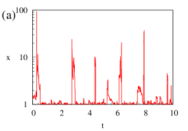
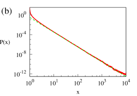
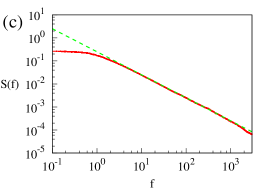
Figure 1: (Color online) (a) Signal generated by SDE with Lévy stable noise (42) with reflective boundaries at $x=x_{\mathrm{min}}$ and $x=x_{\mathrm{max}}$. (b) Steady state PDF $P_{0}(x)$ of the signal. The dashed green line shows the slope $x^{-3}$. (c) Power spectral density $S(f)$ of the signal. The dashed green line shows the slope $1/f$. Parameters used are $x_{\mathrm{min}}=1$, $x_{\mathrm{max}}=10^{4}$, $\sigma=1$.

When $\alpha=1$, $\lambda=3$ and $\eta=9/4$, the SDE (19) is

$$dx=-\sigma x^{9/4}dt+\sigma x^{9/4}dL_{t}^{1}\,.$$ (42)

The results obtained numerically solving this equation with reflective boundaries at $x=x_{\mathrm{min}}$ and $x=x_{\mathrm{max}}$ are shown in Fig. 1. A sample of the generated signal is shown in Fig. 1a. The signal exhibits peaks or bursts, corresponding to the large deviations of the variable $x$. Comparison of the steady state PDF $P_{0}(x)$ and the PSD $S(f)$ with the analytical estimations is presented in Fig. 1b and Fig. 1c. There is quite good agreement of the numerical results with the analytical expressions. In Fig. 1b we see that near the reflecting boundaries the steady state PDF deviates from the power law prediction. This increase of the steady state PDF near boundaries is typical for equations with Lévy stable noise having $\alpha<2$ Denisov et al. (2008). The behavior of the steady state PDF near the reflecting boundaries is similar to the behavior of the analytical expression obtained in Ref. Denisov et al. (2008) for the simplest stochastic differential equation Lévy stable noise having constant noise amplitude and zero drift.

A numerical solution of the equations confirms the presence of the frequency region for which the PSD has $1/f$ dependence. The width of this region can be increased by increasing the ration between the minimum and the maximum values of the stochastic variable $x$. In addition, the region in the PSD with the power law behavior depends on $\alpha$ and the exponent $\eta$: the width increases with increasing the difference $\eta-1$ and increasing $\alpha$; when $\eta=1$ then this width is zero. Such behavior is correctly predicted by Eq. (38).

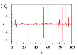
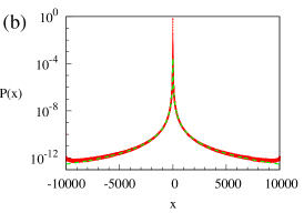
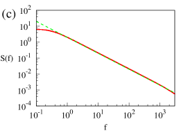
Figure 2: (Color online) (a) Signal generated by SDE with Lévy stable noise (47). (b) Steady state PDF $P_{0}(x)$ of the signal. The dashed green line shows the dependence on $x$ proportional to $|x|^{-3}$. (c) Power spectral density $S(f)$ of the signal. The dashed green line shows the slope $1/f$. Parameters used are $x_{0}=1$, $x_{\mathrm{max}}=10^{4}$, $\sigma=1$.

Similar schemes of numerical solution we use also for SDEs (30) and (31). Euler’s approximation with variable step of integration

$$h_{k}=\frac{\kappa^{\alpha}}{\sigma^{\alpha}}(x_{0}^{2}+x_{k}^{2})^{-\frac{\alpha}{2}(\eta-1)}$$ (43)

transforms SDE (30) to the difference equation

$$x_{k+1}=x_{k}+\kappa^{\alpha}\gamma x_{k}+\frac{\kappa}{\sigma}\sqrt{x_{0}^{2}+x_{k}^{2}}\xi_{k}^{\alpha}\,.$$ (44)

For SDE (31) we use the variable step of integration

$$h_{k}=\frac{\kappa^{\alpha}}{\sigma^{\alpha}}(x_{0}^{\alpha}+|x_{k}|^{\alpha})^{-(\eta-1)}$$ (45)

resulting in the difference equation

$$x_{k+1}=x_{k}+\kappa^{\alpha}\gamma x_{k}+\frac{\kappa}{\sigma}(x_{0}^{\alpha}+|x_{k}|^{\alpha})^{\frac{1}{\alpha}}\xi_{k}^{\alpha}\,.$$ (46)

Here $\kappa\ll 1$ is a small parameter. Reflective boundaries at $x=\pm x_{\mathrm{max}}$ we include using the projection method.

When $\alpha=1$ , $\lambda=3$ and $\eta=5/2$, the SDE (30) with the coefficient $\gamma$ given by Eq. (26) is

$$dx=-\sigma(x_{0}^{2}+x^{2})^{3/4}xdt+(x_{0}^{2}+x^{2})^{5/4}dL_{t}^{1}\,.$$ (47)

The results obtained numerically solving this equation with reflective boundaries at $x=\pm x_{\mathrm{max}}$ are shown in Fig. 2. A sample of the generated signal is shown in Fig. 2a. Comparison of the steady state PDF $P_{0}(x)$ and the PSD $S(f)$ with the analytical estimations is presented in Fig. 2b and Fig. 2c. There is quite good agreement of the numerical results with the analytical expressions. As in the case with only positive values of $x$, we see in Fig. 1b we see the increase of the steady state PDF near the reflecting boundaries $x=\pm x_{\mathrm{max}}$ in comparison to the power law prediction. Numerical solution of Eq. (47) confirms the presence of the frequency region where the PSD has $1/f^{\beta}$ dependence.

V Discussion

Lévy flights have been modeled using Langevin equation with various subharmonic potentials and additive Lévy stable noise Jespersen et al. (1999); Brockmann and Sokolov (2002); Chechkin et al. (2002); Brockmann and Geisel (2003b). Proposed SDE (19) contains multiplicative Lévy stable noise and is a generalization of previous attempts to model Lévy flights. This SDE can be used to investigate Lévy flights in non-equilibrium and non-homogeneous environments, like porous media and some cases of polymer chains Brockmann and Geisel (2003a); Lomholt et al. (2005). If specific conditions given by Eq. (20) are satisfied, our model generates Lévy flights exhibiting $1/f$ noise. The drift term $a(x)$ in Eq. (19) represents a subharmonic external force effecting the particle. Lévy flights in subharmonic potentials lead to various interesting phenomena such as stochastic resonance in singe well potential Dybiec (2009). The power law dependence of the diffusion coefficient $b^{2}(x)$ on the stochastic variable $x$ can be traced to the existence of the energy flux due to temperature gradient in a bath. Long jumps leading to Lévy stable noise can arise from a complex scale free structure of the bath as is in the case of enzyme diffusion on a polymer Brockmann and Geisel (2003a). There are suggestions that the non-homogeneity of the bath can be described by the dependence of the diffusion coefficient on the particle coordinate $x$ Srokowski (2009a) and Lévy stable noise arises from the bath not being in an equilibrium.

In the case of Gaussian noise ($\alpha=2$) nonlinear SDE (19) that generates signal with $1/f$ spectrum can be obtained from various models. One of those models is a signal consisting form a sequence of pulses with a Brownian motion of the inter-pulse durations Kaulakys and Ruseckas (2004); Kaulakys et al. (2006). This suggests that our more general form of the SDE could be obtained from some kind of Lévy motion of the inter-pulse durations. However, we were unable to show this due to the complexity of Itô formula in case of equations driven by Lévy process Jacobs (2010). The special case of Eq. (19) for free particle ($a(x)=0$) with Lévy stable noise having $\alpha<2$ has been derived from coupled continuous time random walk (CTRW) models Srokowski and Kaminska (2006), when jumping rate $\nu$ of CTRW process depends on signal intensity as $\nu(x)=x^{\alpha\eta}$, $x>0$. However, such derivation is quite complex and does little to help the understanding what kind of physical phenomena can be approximated by multiplicative Lévy stable noise. Thus instead of searching for underlying models in this article we have chosen an simpler approach: we have derived nonlinear SDEs using a simple reasoning about scaling properties of the steady state PDF.

Taking into account of the scaling properties of the signal is one of the advantages of our model. In many theoretical models, such as diffusion of the particle in a fractal turbulence Takayasu (1984), ecological population density with fluctuating volume of resources Dubkov (2012), dynamics of two competing species La Cognata et al. (2010) and tumor growth Jiang et al. (2012), an existence of Lévy stable noise instead of Gaussian noise is simply assumed. Such assumption might be incorrect, because the change of statistical properties of the noise change the scaling properties of the signal. In order to preserve original scaling properties of the signal the drift $a(x)$ or diffusion $b^{2}(x)$ coefficients must be changed as well. The required drift coefficient $a(x)$ can be found similarly as in Section II. The scaling properties can be extracted from time series using fluctuation analysis methods Weron et al. (2005).

In summary, we have proposed nonlinear SDEs with Lévy stable noise and generating signals exhibiting $1/f$ noise in any desirably wide range of frequency. Proposed SDEs (19), (30) and (31) are a generalization of nonlinear SDEs driven by Gaussian noise and generating signals with $1/f$ PSD. The generalized equations can be obtained by replacing the Gaussian noise with the Lévy stable noise and changing the drift term to preserve statistical properties of the generated signal. We have investigated two cases: in the first case the stochastic variable can acquire only positive values (SDE (19)), in the second case the stochastic variable can also be negative (SDEs (30) and (31)). In contrast to the SDEs with the Gaussian noise, the constant in the drift term, given by Eqs. (18) and (26), is different in those two cases and becomes the same only for $\alpha=2$.

References

- Marandet et al. (2003) Y. Marandet, H. Capes, L. Godbert-Mouret, R. Guirlet, M. Koubiti, and R. Stamm, Commun. Nonlinear. Sci. Commun. 8, 469 (2003).
- Mercadier et al. (2009) N. Mercadier, W. Guerin, M. Chevrollier, and R. Kaiser, Nat. Phys. 5, 602 (2009).
- Takayasu (1984) H. Takayasu, Prog. Theor. Phys. 72, 471 (1984).
- Min et al. (1996) I. A. Min, I. Mezic, and A. Leonard, Phys. Fluids 8, 1169 (1996).
- Guantes et al. (2001) R. Guantes, J. L. Vega, and S. Miret-Artés, Phys. Rev. B 64, 245415 (2001).
- Luedtke and Landman (1999) W. D. Luedtke and U. Landman, Phys. Rev. Lett. 82, 3835 (1999).
- Marksteiner et al. (1996) S. Marksteiner, K. Ellinger, and P. Zoller, Phys. Rev. A 53, 3409 (1996).
- Fogedby (1994a) H. C. Fogedby, Phys. Rev. Lett. 73, 2517 (1994a).
- Jespersen et al. (1999) S. Jespersen, R. Metzler, and H. C. Fogedby, Phys. Rev. E 59, 2736 (1999).
- Chechkin et al. (2002) A. Chechkin, V. Gonchar, J. Klafter, and R. M. L. Tanatarov, Chem. Phys. 284, 233 (2002).
- Eliazar and Klafter (2003) I. Eliazar and J. Klafter, J. Stat. Phys. 111, 739 (2003).
- Denisov et al. (2008) S. I. Denisov, W. Horsthemke, and P. Hänggi, Phys. Rev. E 77, 061112 (2008).
- Srokowski (2009a) T. Srokowski, Phys. Rev. E 79, 040104(R) (2009a).
- Dubkov (2012) A. Dubkov, Acta Phys. Pol. B 43, 935 (2012).
- Schertzer et al. (2001) D. Schertzer, M. Larchev, J. Duan, V. V. Yanovsky, and S. Lovejoy, J. Math. Phys 42, 200 (2001).
- Srokowski (2009b) T. Srokowski, Phys. Rev. E 80, 051113 (2009b).
- Lomholt et al. (2005) M. A. Lomholt, T. Ambjörnsson, and R. Metzler, Phys. Rev. Lett. 95, 260603 (2005).
- Srokowski and Kaminska (2006) T. Srokowski and A. Kaminska, Phys. Rev. E 74, 021103 (2006).
- Brockmann and Geisel (2003a) D. Brockmann and T. Geisel, Phys. Rev. Lett. 91, 048303 (2003a).
- Brockmann and Sokolov (2002) D. Brockmann and I. Sokolov, Chem. Phys. 284, 409 (2002).
- Brockmann and Geisel (2003b) D. Brockmann and T. Geisel, Phys. Rev. Lett. 90, 170601 (2003b).
- Ward and Greenwood (2007) L. M. Ward and P. E. Greenwood, Scholarpedia 2, 1537 (2007).
- Weissman (1988) M. B. Weissman, Rev. Mod. Phys. 60, 537 (1988).
- Barabasi and Albert (1999) A. L. Barabasi and R. Albert, Science 286, 509 (1999).
- Gisiger (2001) T. Gisiger, Biol. Rev. 76, 161 (2001).
- Wagenmakers et al. (2004) E.-J. Wagenmakers, S. Farrell, and R. Ratcliff, Psychonomic Bull. Rev. 11, 579 (2004).
- Szabo and Fath (2007) G. Szabo and G. Fath, Phys. Rep. 446, 97 (2007).
- Castellano et al. (2009) C. Castellano, S. Fortunato, and V. Loreto, Rev. Mod. Phys. 81, 591 (2009).
- Johnson (1925) J. B. Johnson, Phys. Rev. 26, 71 (1925).
- Schottky (1926) W. Schottky, Phys. Rev. 28, 74 (1926).
- Kaulakys and Alaburda (2009) B. Kaulakys and M. Alaburda, J. Stat. Mech. 2009, P02051 (2009).
- Balandin (2013) A. A. Balandin, Nature Nanotechnology 8, 549 (2013).
- Kogan (2008) S. Kogan, Electronic Noise and Fluctuations in Solids (Cambrige Univ. Press, 2008).
- Li and Zhao (2012) M. Li and W. Zhao, Math. Probl. Egin. 2012, 23 (2012).
- Orlyanchik et al. (2008) V. Orlyanchik, M. B. Weissman, M. A. Torija, M. Sharma, and C. Leighton, Phys. Rev. B 78, 094430 (2008).
- Melkonyan (2010) S. V. Melkonyan, Physica B 405, 379 (2010).
- McWhorter (1957) A. L. McWhorter, Semiconductor Surface Physics, edited by R. H. Kingston (University of Pennsylvania Press, Philadelphia, 1957) pp. 207–228.
- Bak et al. (1987) P. Bak, C. Tang, and K. Wiesenfeld, Phys. Rev. Lett. 59, 381 (1987).
- Jensen et al. (1989) H. J. Jensen, K. Christensen, and H. C. Fogedby, Phys. Rev. B 40, 7425 (1989).
- Kertesz and Kiss (1990) J. Kertesz and L. B. Kiss, J. Phys. A: Math. Gen. 23, L433 (1990).
- Kaulakys and Meškauskas (1998) B. Kaulakys and T. Meškauskas, Phys. Rev. E 58, 7013 (1998).
- Kaulakys (1999) B. Kaulakys, Phys. Lett. A 257, 37 (1999).
- Kaulakys (2000) B. Kaulakys, Microel. Reliab. 40, 1787 (2000).
- Kaulakys et al. (2005) B. Kaulakys, V. Gontis, and M. Alaburda, Phys. Rev. E 71, 051105 (2005).
- Kaulakys and Ruseckas (2004) B. Kaulakys and J. Ruseckas, Phys. Rev. E 70, 020101(R) (2004).
- Kaulakys et al. (2006) B. Kaulakys, J. Ruseckas, V. Gontis, and M. Alaburda, Physica A 365, 217 (2006).
- Ruseckas and Kaulakys (2010) J. Ruseckas and B. Kaulakys, Phys. Rev. E 81, 031105 (2010).
- Ruseckas and Kaulakys (2011) J. Ruseckas and B. Kaulakys, Phys. Rev. E 84, 051125 (2011).
- Ruseckas et al. (2011) J. Ruseckas, B. Kaulakys, and V. Gontis, EPL 96, 60007 (2011).
- Gontis et al. (2010) V. Gontis, J. Ruseckas, and A. Kononovicius, Physica A 389, 100 (2010).
- Mathiesen et al. (2013) J. Mathiesen, L. Angheluta, P. T. H. Ahlgren, and M. H. Jensen, PNAS 110, 17259 (2013).
- Fogedby (1994b) H. C. Fogedby, Phys. Rev. E 50, 1657 (1994b).
- Fogedby (1998) H. C. Fogedby, Phys. Rev. E 58, 1690 (1998).
- Janicki and Weron (1994) A. Janicki and A. Weron, A Simulation and Chaotic Behaviour of -Stable Stochastic Processes (Dekker, New York, 1994).
- Weron et al. (2005) A. Weron, K. Burnecki, S. Mercik, and K. Weron, Phys. Rev. E 71, 016113 (2005).
- Ditlevsen (1999) P. D. Ditlevsen, Phys. Rev. E 60, 172 (1999).
- Samko et al. (1993) S. G. Samko, A. A. Kilbas, and O. I. Marichev, Fractional Integrals and Derivatives: Theory and Applications (Gordon and Breach, New York, 1993).
- Ruseckas and Kaulakys (2013) J. Ruseckas and B. Kaulakys, Chaos 23, 023102 (2013).
- Ruseckas and Kaulakys (2014) J. Ruseckas and B. Kaulakys, (2014), arXiv:1402.2523 [cond-mat.stat-mech] .
- Gardiner (2004) C. W. Gardiner, Handbook of Stochastic Methods for Physics, Chemistry and the Natural Sciences (Springer-Verlag, Berlin, 2004).
- Liu (1995) Y. J. Liu, Mathematics and Computers in Simulation 38, 103 (1995).
- Pettersson (1995) R. Pettersson, Stochastic Processes and their Applications 59, 295 (1995).
- Dybiec (2009) B. Dybiec, Phys. Rev. E 80, 041111 (2009).
- Jacobs (2010) K. Jacobs, Stochastic Processes for Physicists: Understanding Noisy Systems (Cambridge University Press, 2010).
- La Cognata et al. (2010) A. La Cognata, D. Valenti, A. A. Dubkov, and B. Spagnolo, Phys. Rev. E 82, 011121 (2010).
- Jiang et al. (2012) L. Jiang, X. Luo, D. Wu, and S. Zhu, Mod. Phys. Lett. B 26, 1250149 (2012).