Ground States of a Bose-Hubbard Ladder in an Artificial Magnetic Field:
Field-Theoretical Approach

Abstract

We consider a Bose-Hubbard ladder subject to an artificial magnetic flux and discuss its different ground states, their physical properties, and the quantum phase transitions between them. A low-energy effective field theory is derived, in the two distinct regimes of a small and large magnetic flux, using a bosonization technique starting from the weak-coupling limit. Based on this effective field theory, the ground-state phase diagram at a filling of one particle per site is investigated for a small flux and for a flux equal to $\pi$ per plaquette. For $\pi$-flux, this analysis reveals a tricritical point which has been overlooked in previous studies. In addition, the Mott insulating state at a small magnetic flux is found to display Meissner currents.

I Introduction

Recent developments in ultra-cold atom physics allow for studies of a wide range of many-body quantum systems of bosons, fermions and their mixtures, involving strong correlations and/or frustration. One of the remarkable recent advances is the so-called artificial gauge fields, Dalibard et al. (2011) which allow one to generate spin-orbit couplings and magnetic fields, opening the way for example to quantum Hall and spin Hall effects. These effects are also related to studies on topological phases of matters. In addition, the control of interactions between atoms by the Feshbach resonance technique allows for the controlled study of quantum systems under the combined effects of an artificial gauge field and strong correlations.

The key to artificial gauge fields is Berry’s phases Berry (1984) tuned by atom-light interactions, Dum and Olshanii (1996) in which atoms acquire a geometric phase in their motion because of an adiabatic spatial change of the dressed states. Using Raman transitions based on these ideas, the synthesis of an effective magnetic field Lin et al. (2009) and spin-orbit coupling Lin et al. (2011); Wang et al. (2012); Cheuk et al. (2012) have been experimentally achieved in Bose condensates of ⁸⁷Rb atoms, and the spin-Hall effect in Bose condensates has been also successfully observed Beeler et al. (2013).

The realization of artificial gauge fields in optical lattice potentials has also been intensively discussed. The pioneering theory making use of photo-assisted tunneling techniques has been established by Jaksch and Zoller Jaksch and Zoller (2003). Subsequently other schemes for effective uniform magnetic fields Sørensen et al. (2005); Mueller (2004) and for staggered magnetic fields Lim et al. (2008, 2010) have also been proposed. In experiments, several types of artificial magnetic fields using photo-assisted tunneling have been subsequently realized in recent years: effective magnetic fluxes inhomogeneously set in stripes Aidelsburger et al. (2011, 2013a), uniform magnetic fluxes Miyake et al. (2013), and spin-orbit couplings without spin flips Kennedy et al. (2013); Aidelsburger et al. (2013b) in two-dimensional optical lattice systems. In addition to the above realizations, other schemes for artificial gauge fields have been invented using Zeeman lattice techniques Jiménez-García et al. (2012) and shaking of optical lattice potentials Struck et al. (2012); Simonet, J. et al. (2013); Struck et al. (2013).

Optical lattices also allow for the control of dimensionality, so that one-dimensional quantum systems can be realized. A quasi-one-dimensional “ladder” geometry plays the role of a minimal model for studying the effect of gauge fields. In these low-dimensional systems, the whole range of interaction strengths from weak to strong coupling can be investigated using powerful numerical and analytic techniques, such as bosonization and the density-matrix renormalization group (DMRG). Because of the peculiar critical nature of Tomonaga-Luttinger (TL) liquids which describe their low-energy properties, such quasi-one-dimensional quantum systems subject to artificial gauge fields or high magnetic fields are expected to display interesting phenomena. In studies on ladder systems subjected to magnetic fields, fermion systems have been discussed in the context of strongly correlated electron systems Carr et al. (2006); Jaefari and Fradkin (2012); Carr et al. (2006); Roux et al. (2007); Schollwöck et al. (2003). The study of bosonic ladders subject to magnetic fields has also been motivated by the Josephson junction ladders and ultra-cold Bose atoms in optical lattices Denniston and Tang (1995); Kardar (1986); Granato (1990); Nishiyama (2000); Orignac and Giamarchi (2001); Petrescu and Le Hur (2013); Dhar et al. (2013, 2012); Crépin et al. (2011); Tovmasyan et al. (2013). In addition to common features of Bose-Hubbard models such as a one-dimensional superfluid (SF), Mott insulator (MI), and phase transition between them, the bosonic ladders exhibit interesting phenomena induced by the magnetic field: chiral superfluid phases (CSF) and chiral Mott insulating phases (CMI) displaying Meissner currents Orignac and Giamarchi (2001); Dhar et al. (2013, 2012); Petrescu and Le Hur (2013). Attention to the topic of bosonic ladders subject to an artificial magnetic field has been reinforced recently by the first experimental realization of such a system. Atala et al. (2014)

In this article, we study the low-energy physics of Bose-Hubbard ladders subject to an artificial uniform magnetic flux, from the viewpoint of field theory. So far, field theoretical approaches to bosonic ladder systems have usually considered starting with the strong coupling limit, in which the rung hopping is treated perturbatively Donohue and Giamarchi (2001); Orignac and Giamarchi (2001); Petrescu and Le Hur (2013) In contrast, we derive an effective field theory from a weak coupling perspective, in which the effect of a rung hopping is fully taken into account, and the interaction is included perturbatively. In this approach, typical strong correlation phenomena such as the MI state and the MI-SF phase transition can nonetheless be investigated, by taking into account backscattering and umklapp scattering processes. The low-energy effective field theories in the two cases of a large and small magnetic flux are separately derived, for an arbitrary filling. In addition we also apply the constructed effective field theory and investigate the ground-state phase diagram in two limiting cases, namely that of a large magnetic flux equal to $\pi$ per plaquette, and that of a small magnetic flux, with one particle per site. For the $\pi$ magnetic flux, we compare our phase diagram to the one previously obtained numerically in Ref. Dhar et al. (2012), and all the phases found there are well described by our approach. Furthermore, more importantly, the presence of a tricritical point in the phase diagram is predicted by the analysis presented here, which has not been emphasized previously. In the limit of a small magnetic flux, we show that a SF state with Meissner current appears, and transits to the MI state for strong interactions. In addition we also find that the Meissner current can survive also in the MI state while the system is fully gapped. A similar fully gapped charge-ordered state with Meissner currents has also been found for the different filling of one particle per two sites by Petrescu and Le Hur Petrescu and Le Hur (2013).

This paper is organized as follows. In Sec. II we first define the considered Bose-Hubbard ladder with a magnetic flux. Next we analyze the single-particle band structure in the non-interacting case in Sec. II.1, and derive the general form of the low-energy effective field theory for a large magnetic flux in Sec. II.2, and for a small magnetic flux in Sec. II.3. Furthermore, based on the derived field theory, we investigate the ground-state phase diagrams in Sec. III. A summary and conclusion are provided in Sec. IV. In Appendix A, the mean-field analysis which is used to construct the effective field theories is presented.

II Model and effective theory

Let us define the Bose-Hubbard ladder Hamiltonian with an applied uniform artificial magnetic field,

$$H =H_{0}+H_{\mathrm{loc}},$$ (1)

$$H_{0} =-J\sum_{p=1,2}\sum_{j}\left[e^{iA^{\parallel}_{j,p}}b^{\dagger}_{j+1,p}b_{j,p}+\mathrm{h.c.}\right]$$

$$\quad-J_{\perp}\sum_{j}\left[e^{iA^{\perp}_{j}}b^{\dagger}_{j,1}b_{j,2}+\mathrm{h.c.}\right],$$ (2)

$$H_{\mathrm{loc}} =\sum_{j}\sum_{p=1,2}\left[-\mu n_{j,p}+\frac{U}{2}n_{j,p}\left(n_{j,p}+1\right)\right],$$ (3)

where $n_{j,p}=b^{\dagger}_{j,p}b_{j,p}$ is a number operator, and the index $p=1,2$ denotes the upper and lower chain, respectively. The model Hamiltonian is schematically illustrated in Fig. 1.

Figure 1: The Bose-Hubbard ladder Hamiltonian considered in this paper. Due to the magnetic field, hopping involves a phase factor associated with the corresponding gauge field. The phases gained in the hopping processes are displayed, corresponding to the gauge choice defined by Eq. (5).

This model has the two different hoppings, intrachain $J>0$ and interchain $J_{\perp}>0$, and only a repulsive on-site Hubbard interaction $U>0$ is considered. The artificial magnetic field is introduced via the Peierls substitution, and the corresponding gauge field along the chain direction on the chain $p$, and along the rung direction are denoted by $A^{\parallel}_{j,p}$ and $A^{\perp}_{j}$, respectively. This produces the applied artificial magnetic flux $\phi$ piercing a plaquette as

$$\oint_{\Box}\bm{A}\cdot d\bm{l}=A^{\parallel}_{j,1}-A^{\perp}_{j+1}-A^{\parallel}_{j,2}+A^{\perp}_{j}=\phi.$$ (4)

In this paper, we choose the following gauge:

$$\left\{\begin{aligned} &A^{\parallel}_{j,1}=\phi/2,\\ &A^{\parallel}_{j,2}=-\phi/2,\\ &A^{\perp}_{j}=0,\end{aligned}\right.$$ (5)

which obviously obeys Eq. (4). The Hamiltonian (1) is invariant under the transformation, $(\phi,b_{j,1},b_{j,2})\rightarrow(-\phi,b_{j,2},b_{j,1})$. Thus the magnetic flux $\phi$ to be considered can be primitively reduced, and we restrict the magnetic flux to be $0<\phi\leq\pi$ throughout this paper.

II.1 Single-particle energy band structure

Let us look at the single-particle spectrum. The single-particle Hamiltonian (2) is easily diagonalized by the following unitary transformation as

$$\left\{\begin{aligned} &b_{1}(k)=v_{k}\alpha(k)+u_{k}\beta(k),\\ &b_{2}(k)=-u_{k}\alpha(k)+v_{k}\beta(k),\\ \end{aligned}\right.$$ (6)

where $b_{p}(k)$ with $p=1,2$ is a Fourier transformation of $b_{j,p}$. The coefficients are given as

$$\left\{\begin{aligned} u_{k}&=\sqrt{\frac{1}{2}\left(1-\frac{\sin(\phi/2)\sin{k}}{\sqrt{(J_{\perp}/2J)^{2}+\sin^{2}(\phi/2)\sin^{2}{k}}}\right)},\\ v_{k}&=\sqrt{\frac{1}{2}\left(1+\frac{\sin(\phi/2)\sin{k}}{\sqrt{(J_{\perp}/2J)^{2}+\sin^{2}(\phi/2)\sin^{2}{k}}}\right)}.\end{aligned}\right.$$ (7)

Consequently the single-particle Hamiltonian (2) has a two-band structure:

$$H_{0} =\sum_{k}\left[E_{+}(k)\alpha^{\dagger}(k)\alpha(k)+E_{-}(k)\beta^{\dagger}(k)\beta(k)\right],$$ (8)

with the single-particle energy bands being

$$E_{\pm}(k) =-2J\cos\left(\frac{\phi}{2}\right)\cos{k}$$

$$\quad\pm\sqrt{J_{\perp}^{2}+(2J)^{2}\sin^{2}\left(\frac{\phi}{2}\right)\sin^{2}{k}}.$$ (9)

The energy dispersions $E_{\pm}(k)$ correspond to the upper and lower band, respectively. The band structures for certain values of $\phi$ and $J_{\perp}/J$ are shown in Fig. 2.

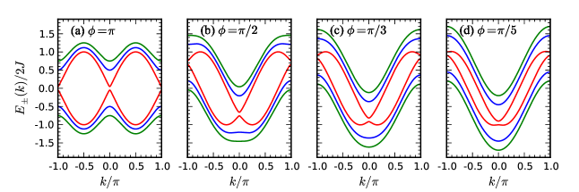
Figure 2: (Color online) The single-particle energy bands of the two-leg ladder with a uniform magnetic flux: (a) $\phi=\pi$, (b) $\phi=\pi/2$, (c) $\phi=\pi/3$ and (d) $\phi=\pi/5$. The red, blue and green lines denote $J_{\perp}/2J=0.05$, $0.5$ and $0.75$, respectively. Here only the commensurate magnetic fluxes are shown, but the structure of the spectrum is continuously deformed by varying the flux $\phi$.

Comprehensive results on the dependence of the band structure on the magnetic field $\phi$ and hopping ratio $J_{\perp}/J$ can be found in Refs. Carr et al. (2006); Roux et al. (2007). In addition, the band structure of the Hamiltonian $H_{0}$ is known to be analogous to that of spin-$1/2$ particles with a spin-orbit coupling in the presence of a magnetic field Hügel and Paredes (2014).

The band structure around the lowest energy is the most important feature for low-energy physics, since bosons tend to populate states around energy minima. Thus we focus here only on the features at the bottom of the lower band. In the regime of a large magnetic flux per plaquette the lower band $E_{-}(k)$ has two separate minima, and the corresponding wave numbers $k_{\mathrm{min}}$ at the band minima are given analytically as $k_{\mathrm{min}}=\pm Q$ with

$$Q=\arccos\left[\cot\left(\frac{\phi}{2}\right)\sqrt{\left(\frac{J_{\perp}}{2J}\right)^{2}+\sin^{2}\left(\frac{\phi}{2}\right)}\right],$$ (10)

which is shown in Fig. 3.

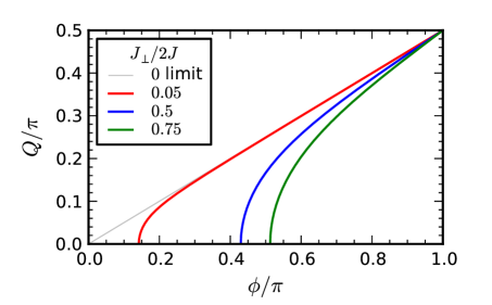
Figure 3: (color online) The position of the momentum corresponding to the band minima, $k_{\min}=\pm Q$, as a function of the magnetic flux per plaquette $\phi$ for several hopping ratios $J_{\perp}/2J$. A finite $Q$ corresponds to the case when the lower band displays two minima, while $Q=0$ means that the band has a single minimum structure. The critical value of the magnetic flux, at which $Q$ becomes zero, increases with $J_{\perp}/J$ as in Eq. (11).

The two band minima are maximally separated for $\phi=\pi$, and located exactly at $k_{\mathrm{min}}=\pm\pi/2$. As the flux $\phi$ decreases, the two minima approach one another, and eventually merge at a critical value of the magnetic flux

$$\phi_{\mathrm{c}}=2\arccos\left[\sqrt{\left(\frac{J_{\perp}}{4J}\right)^{2}+1}-\frac{J_{\perp}}{4J}\right].$$ (11)

A single minimum structure is formed for small $\phi$. On the other hand, the hopping ratio $J_{\perp}/J$ works so as to enlarge the distance between the two bands, and so as to narrow the band width. Thus the increase of the ratio $J_{\perp}/J$ suppresses the height of the barrier between the two minima in the lower band, which also leads to the increase of the critical $\phi_{c}$ with $J_{\perp}/J$. In what follows, we separately consider the two different cases. The first is the case of a sufficiently large magnetic flux $\phi\gg\phi_{\mathrm{c}}$, in which the bottom of the lower band exhibits double minima, and they are clearly separated. The second is the case of a small magnetic flux $\phi<\phi_{c}$, in which the band bottom forms a single minimum structure.

II.2 Effective Hamiltonian for large magnetic flux

Let us derive the low-energy effective theory based on the single-particle spectrum obtained above. For a large enough magnetic flux $\phi\gg\phi_{\mathrm{c}}$, we have a double-minimum structure in the lower energy band, and in the ground state the bosons dominantly populate the two energy minima even in the presence of the interaction. Thus, the spectrum relevant to the low-energy physics can be approximated by expanding the band-structure around the energy minima:

$$E_{-}(k=\pm Q+q)\approx-E_{0}+\frac{q^{2}}{2m^{*}},$$ (12)

where $E_{0}=-E(k=\pm Q)$ and $m^{*}$ are, respectively, a minimum energy offset and effective mass, and they are given as

$$E_{0}=\frac{2J}{\sin\left(\frac{\phi}{2}\right)}\sqrt{\left(\frac{J_{\perp}}{2J}\right)^{2}+\sin^{2}\left(\frac{\phi}{2}\right)},$$ (13)

$$\frac{1}{m^{*}}=\frac{d^{2}E(k=\pm Q)}{dk^{2}}.$$ (14)

The wave number $q$ denotes the variation from the minima $k_{\mathrm{min}}=\pm Q$, and is assumed to be small enough, $q\ll 1$. The minimum energy offset $-E_{0}$ shifts the chemical potential $\mu$ in the Hamiltonian (1). Thus under this long-wave-length approximation we need to fix the chemical potential including this energy offset to reproduce the required density.

Correspondingly to the long-wave-length expansion, the unitary transformation (6) is also approximated as follows. For the upper chain,

$$\left\{\begin{aligned} &b_{1}(k=Q+q)=V_{-}\beta_{+}(q),\\ &b_{1}(k=-Q+q)=V_{+}\beta_{-}(q),\end{aligned}\right.,$$

and for the lower chain,

$$\left\{\begin{aligned} &b_{2}(k=Q+q)=V_{+}\beta_{+}(q),\\ &b_{2}(k=-Q+q)=V_{-}\beta_{-}(q).\end{aligned}\right.,$$

where the weight factors, $V_{+}=u_{-Q}=v_{Q}$ and $V_{-}=u_{Q}=v_{-Q}$, have been introduced, and they are explicitly given as

$$V_{\pm}=\sqrt{\frac{1}{2}\left[1\pm\sqrt{\frac{\sin^{2}(\phi/2)-(J_{\perp}/2J)^{2}\cot^{2}(\phi/2)}{(J_{\perp}/2J)^{2}+\sin^{2}(\phi/2)}}\right]}.$$ (15)

This approximation means that all the energy states except for the low-energy states near the band bottom are projected out.

The approximated boson operators are represented in real space as

$$\left\{\begin{aligned} &b_{j,1}\approx e^{-iQj}V_{-}\beta_{+,j}+e^{iQj}V_{+}\beta_{-,j},\\ &b_{j,2}\approx e^{-iQj}V_{+}\beta_{+,j}+e^{iQj}V_{-}\beta_{-,j},\end{aligned}\right.$$ (16)

which lead to the following representation of the number operators as

$$\left\{\begin{aligned} n_{j,1}&\approx V_{-}^{2}\tilde{n}_{+,j}+V_{+}^{2}\tilde{n}_{-,j}+V_{+}V_{-}\left(e^{i2Qj}\beta_{+,j}^{\dagger}\beta_{-,j}+\mathrm{h.c.}\right),\\ n_{j,2}&\approx V_{+}^{2}\tilde{n}_{+,j}+V_{-}^{2}\tilde{n}_{-,j}+V_{+}V_{-}\left(e^{i2Qj}\beta_{+,j}^{\dagger}\beta_{-,j}+\mathrm{h.c.}\right),\end{aligned}\right.$$ (17)

where the density operators for the separate quadratic energy dispersions have been defined as $\tilde{n}_{\pm,j}=\beta_{\pm,j}^{\dagger}\beta_{\pm,j}$. The above representation of the field operators in the long-wave-length approximation has a similar form to that of fermions. Namely the wave numbers $\pm Q$ giving the minima of the energy band are analogous to Fermi points.

From the above, the Hamiltonian in the long-wave-length-approximation are derived. The single particle Hamiltonian (2) is rewritten as

$$H_{0}\approx-E_{0}\sum_{j,\sigma=\pm}\tilde{n}_{\sigma,j}+\sum_{q,\sigma=\pm}\frac{q^{2}}{2m^{*}}\beta_{\sigma,q}^{\dagger}\beta_{\sigma,q},$$ (18)

where $\beta_{\sigma}(q)$ is a Fourier transform of $\beta_{\sigma,j}$. Using the representation of Eq. (17), the local Hamiltonian (3) is rewritten as

$$H_{\mathrm{loc}} \approx-\left(\mu+\frac{U}{2}-UV_{+}^{2}V_{-}^{2}\right)\sum_{j,\sigma=\pm}\tilde{n}_{\sigma,j}$$

$$\quad+\frac{U}{4}\sum_{j}\biggl{[}\left(1+2V_{+}^{2}V_{-}^{2}\right)\left(\tilde{n}_{+,j}+\tilde{n}_{-,j}\right)^{2}$$

$$\quad+\left(1-6V_{+}^{2}V_{-}^{2}\right)\left(\tilde{n}_{+,j}-\tilde{n}_{-,j}\right)^{2}$$

$$\quad+2V_{+}V_{-}\left(\tilde{n}_{+,j}+\tilde{n}_{-,j}\right)\left(e^{i2Qj}\beta_{+,j}^{\dagger}\beta_{-,j}+\mathrm{H.c.}\right)$$

$$\quad+2V_{+}V_{-}\left(e^{i2Qj}\beta_{+,j}^{\dagger}\beta_{-,j}+\mathrm{H.c.}\right)\left(\tilde{n}_{+,j}+\tilde{n}_{-,j}\right)$$

$$\quad+4V_{+}^{2}V_{-}^{2}\left(e^{i4Qj}\beta_{+,j}^{\dagger}\beta_{+,j}^{\dagger}\beta_{-,j}\beta_{-,j}+\mathrm{H.c.}\right)\biggl{]}.$$ (19)

The $4Q$-oscillating terms in Eq. (19) are regarded as the umklapp scattering between the particles in the two band minima. Thus the commensurability of the magnetic flux is determined by $Q$.

In order to fix the chemical potential for a given particle number per site, $\bar{n}_{p}=\langle{n_{j,p}}\rangle$ ($p=1,2$), we use mean-field analysis. As discussed in Appendix A, the mean-field theory leads to the balanced densities on the chains, $\bar{n}_{1}=\bar{n}_{2}=\tilde{n}_{+}=\tilde{n}_{-}=\bar{n}$ where $\tilde{n}_{\pm}=\langle{\tilde{n}_{\pm,j}}\rangle$, and the density is controlled by the chemical potential as in Eq. (59).

Based on the mean-field solution, we use the following bosonization formula as

$$\left\{\begin{aligned} &\beta_{\pm,j}\sim\sqrt{\bar{n}}e^{i\theta_{\pm}(x_{j})},\\ &n_{\pm,j}\sim\bar{n}-\frac{a}{\pi}\nabla\varphi_{\pm}(x_{j})+2\bar{n}\cos\left[\frac{2\pi\bar{n}}{a}x_{j}-2\varphi_{\pm}(x_{j})\right],\end{aligned}\right.$$ (20)

where we have introduced the continuum coordinate $x_{j}=a\times j$ with the lattice length $a$. Note that from the bosonization formula, the fields $\varphi_{\sigma}$ and $\theta_{\sigma}$ are compactified, respectively, as $\varphi_{\sigma}\sim\varphi_{\sigma}+\pi$ and $\theta_{\sigma}\sim\theta_{\sigma}+2\pi$. In other words, the fields are uniquely defined in the regime,

$$\left\{\begin{aligned} &-\frac{\pi}{2}<\varphi_{\pm}(x)\leq\frac{\pi}{2},\\ &-\pi<\theta_{\pm}(x)\leq\pi,\end{aligned}\right.$$ (21)

Applying Eq. (20) into Eqs. (18) and (19), the low-energy effective Hamiltonian is derived as

$$H_{\mathrm{eff}} =H_{\mathrm{TL}}+\sum_{i=0}^{4}V_{i},$$ (22)

$$H_{\mathrm{TL}} =\frac{v_{\mathrm{s}}}{2\pi}\int\!\!dx\,\left[K_{\mathrm{s}}\left(\nabla\theta_{\mathrm{s}}(x)\right)^{2}+\frac{1}{K_{\mathrm{s}}}\left(\nabla\varphi_{\mathrm{s}}(x)\right)^{2}\right]$$

$$\quad+\frac{v_{\mathrm{a}}}{2\pi}\int\!\!dx\,\left[K_{\mathrm{a}}\left(\nabla\theta_{\mathrm{a}}(x)\right)^{2}+\frac{1}{K_{\mathrm{a}}}\left(\nabla\varphi_{\mathrm{a}}(x)\right)^{2}\right],$$ (23)

$$V_{0} =g_{0}\int\!\!\frac{dx}{a}\,\cos\left(\frac{2Q}{a}x-\sqrt{2}\theta_{\mathrm{a}}(x)\right),$$ (24)

$$V_{1} =g_{1}\int\!\!\frac{dx}{a}\,\cos\left(\frac{4Q}{a}x-\sqrt{8}\theta_{\mathrm{a}}(x)\right),$$ (25)

$$V_{2} =g_{2}\int\!\!\frac{dx}{a}\,\cos\left(\frac{4\pi\bar{n}}{a}x-\sqrt{8}\varphi_{\mathrm{s}}(x)\right),$$ (26)

$$V_{3} =g_{3}\int\!\!\frac{dx}{a}\,\cos\left(\sqrt{8}\varphi_{\mathrm{a}}(x)\right),$$ (27)

$$V_{4} =g_{4}\int\!\!\frac{dx}{a}\,\cos\left(\frac{2\pi\bar{n}}{a}x-\sqrt{2}\varphi_{\mathrm{s}}(x)\right)\cos\left(\sqrt{2}\varphi_{\mathrm{a}}(x)\right),$$ (28)

where the symmetric and antisymmetric fields have been introduced as

$$\left\{\begin{aligned} \varphi_{\mathrm{s},\mathrm{a}}(x)&=\frac{\varphi_{+}(x)\pm\varphi_{-}(x)}{\sqrt{2}},\\ \theta_{\mathrm{s},\mathrm{a}}(x)&=\frac{\theta_{+}(x)\pm\theta_{-}(x)}{\sqrt{2}}.\end{aligned}\right.$$ (29)

The Hamiltonian $H_{\mathrm{TL}}$ stands for that of TL liquids in the symmetric and antisymmetric sectors. Note that due to the redefinition of the fields, the compactification of the fields changes. Oshikawa (2010); Oshikawa et al. (2006); Wong and Affleck (1994) The redefined fields can not be independently compactified, and the identification of the fields are as follows: $\varphi_{\mathrm{s},\mathrm{a}}\sim\varphi_{\mathrm{s},\mathrm{a}}+\pi N_{\mathrm{s},\mathrm{a}}/\sqrt{2}$ with $N_{\mathrm{s}}\equiv N_{\mathrm{a}}$ (modulo $2$), and $\theta_{\mathrm{s},\mathrm{a}}\sim\theta_{\mathrm{s},\mathrm{a}}+\sqrt{2}\pi M_{\mathrm{s},\mathrm{a}}$ with $M_{\mathrm{s}}\equiv M_{\mathrm{a}}$ (modulo $2$). In other words, the symmetric and antisymmetric fields are uniquely defined in the following regime,

$$\left\{\begin{aligned} &-\frac{\pi}{\sqrt{2}}<\varphi_{\mathrm{s}}(x)\pm\varphi_{\mathrm{a}}(x)\leq\frac{\pi}{\sqrt{2}},\\ &-\sqrt{2}\pi<\theta_{\mathrm{s}}(x)\pm\theta_{\mathrm{a}}(x)\leq\sqrt{2}\pi,\end{aligned}\right.$$ (30)

which is important in discussing the degeneracy of the ground states. The parameters introduced are roughly estimated as

$$\left\{\begin{aligned} &v_{\mathrm{s}}\sim a\sqrt{\frac{\bar{n}U}{m^{*}}\left(1+2V_{+}^{2}V_{-}^{2}\right)},\\ &v_{\mathrm{a}}\sim a\sqrt{\frac{\bar{n}U}{m^{*}}\left(1-6V_{+}^{2}V_{-}^{2}\right)},\\ &K_{\mathrm{s}}\sim\pi\sqrt{\frac{\bar{n}/m^{*}U}{1+2V_{+}^{2}V_{-}^{2}}},\\ &K_{\mathrm{a}}\sim\pi\sqrt{\frac{\bar{n}/m^{*}U}{1-6V_{+}^{2}V_{-}^{2}}},\\ &g_{0}\sim 4\bar{n}^{2}UV_{+}V_{-},\\ &g_{1}\sim 2\bar{n}^{2}UV_{+}^{2}V_{-}^{2},\\ &g_{2}\sim 8\bar{n}^{2}UV_{+}^{2}V_{-}^{2},\\ &g_{3}\sim 8\bar{n}^{2}UV_{+}^{2}V_{-}^{2},\\ &g_{4}\sim 2\bar{n}^{2}U\left(1+V_{+}^{2}V_{-}^{2}\right),\end{aligned}\right.$$ (31)

where $V_{+}^{2}V_{-}^{2}=\frac{1}{4}\left(\frac{J_{\perp}}{2J}\right)^{2}/\sin^{2}\left(\frac{\phi}{2}\right)\left[\left(\frac{J_{\perp}}{2J}\right)^{2}+\sin^{2}\left(\frac{\phi}{2}\right)\right]$. The above estimation is valid for a finite but sufficiently small interaction $U\ll J_{\perp}$ since a small interaction preserves the nature of the two minima in the single particle spectrum. At stronger coupling, the parameters will be strong influenced by the renormalization effect due to the irrelevant terms omitted in Eq. (22). However, the following qualitative tendency of the parameters controlled by the microscopic parameters is expected to be captured. In the limit of decoupled chains $J_{\perp}\rightarrow 0$, the velocities $v_{\mathrm{s},\mathrm{a}}$ and Luttinger parameters $K_{\mathrm{s},\mathrm{a}}$ in the symmetric and antisymmetric sectors become identical: $v_{\mathrm{s}}/v_{\mathrm{a}}\rightarrow 1$, and $K_{\mathrm{s}}/K_{\mathrm{a}}\rightarrow 1$ as $J_{\perp}/J\rightarrow 0$. For the finite rung hopping $J_{\perp}$, $K_{\mathrm{s}}/K_{\mathrm{a}}<1$ and $v_{\mathrm{s}}/v_{\mathrm{a}}>1$. In addition, the velocities and Luttinger parameters are controlled, respectively, to be enhanced and suppressed by the increase of the interaction $U$.

It is worthwhile showing the bosonized form of the physical quantity operators, which is useful when we discuss the physical meaning of the ordered phases caused by the lock of the fields $\varphi_{\mathrm{s},\mathrm{a}}$ and $\theta_{\mathrm{s},\mathrm{a}}$. The density operators are represented in the bosonized form as

$$n_{j,1} \sim\bar{n}-\frac{a}{\pi}\left[V_{-}^{2}\nabla\varphi_{+}(x)+V_{+}^{2}\nabla\varphi_{-}(x)\right]$$

$$\quad+2\bar{n}\biggr{[}V_{-}^{2}\cos\left(\frac{2\pi\bar{n}}{a}x-2\varphi_{+}(x)\right)$$

$$\quad\qquad\qquad+V_{+}^{2}\cos\left(\frac{2\pi\bar{n}}{a}x-2\varphi_{-}(x)\right)\biggl{]}$$

$$\quad+2\bar{n}V_{+}V_{-}\cos\left(\frac{2Q}{a}x-\sqrt{2}\theta_{\mathrm{a}}(x)\right),$$ (32)

$$n_{j,2} \sim\bar{n}-\frac{a}{\pi}\left[V_{+}^{2}\nabla\varphi_{+}(x)+V_{-}^{2}\nabla\varphi_{-}(x)\right]$$

$$\quad+2\bar{n}\biggl{[}V_{+}^{2}\cos\left(\frac{2\pi\bar{n}}{a}x-2\varphi_{+}(x)\right)$$

$$\quad\qquad\qquad+V_{-}^{2}\cos\left(\frac{2\pi\bar{n}}{a}x-2\varphi_{-}(x)\right)\biggr{]}$$

$$\quad+2\bar{n}V_{+}V_{-}\cos\left(\frac{2Q}{a}x-\sqrt{2}\theta_{\mathrm{a}}(x)\right).$$ (33)

The current operators are defined as $j^{(\parallel)}_{p,j}=-\partial{H}/\partial{A^{(\parallel)}_{j,p}}$ at the $j$th site on the $p$th chain, and $j^{\perp}_{j}=-\partial{H}/\partial{A^{(\perp)}_{j}}$ on the $j$th rung. Thus the bosonized form are given as

$$j^{(\parallel)}_{j,1} \sim 2\bar{n}J\biggl{[}V_{+}^{2}\sin\left(Q-\frac{\phi}{2}\right)-V_{-}^{2}\sin\left(Q+\frac{\phi}{2}\right)$$

$$\quad+aV_{-}^{2}\cos\left(Q+\frac{\phi}{2}\right)\nabla\theta_{+}(x)$$

$$\quad+aV_{+}^{2}\cos\left(Q-\frac{\phi}{2}\right)\nabla\theta_{-}(x)$$

$$\quad-2V_{+}V_{-}\sin\left(\frac{\phi}{2}\right)\cos\left(\frac{Q}{a}(2x+a)-\sqrt{2}\theta_{\mathrm{a}}(x)\right)\biggr{]},$$ (34)

$$j^{(\parallel)}_{j,2} \sim-2\bar{n}J\biggl{[}V_{+}^{2}\sin\left(Q-\frac{\phi}{2}\right)-V_{-}^{2}\sin\left(Q+\frac{\phi}{2}\right)$$

$$\quad-aV_{+}^{2}\cos\left(Q-\frac{\phi}{2}\right)\nabla\theta_{+}(x)$$

$$\quad-aV_{-}^{2}\cos\left(Q+\frac{\phi}{2}\right)\nabla\theta_{-}(x)$$

$$\quad-2V_{+}V_{-}\sin\left(\frac{\phi}{2}\right)\cos\left(\frac{Q}{a}(2x+a)-\sqrt{2}\theta_{\mathrm{a}}(x)\right)\biggr{]},$$ (35)

$$j^{(\perp)}_{j} \sim 2\bar{n}J_{\perp}\left(V_{+}^{2}-V_{-}^{2}\right)\sin\left(\frac{2Q}{a}x-\sqrt{2}\theta_{\mathrm{a}}(x)\right).$$ (36)

Here in order to somewhat simplify the expression of the density and current operators, we have mixed the notation of $\varphi_{\pm}$ and $\theta_{\pm}$ with that of $\varphi_{\mathrm{s},\mathrm{a}}$ and $\theta_{\mathrm{s},\mathrm{a}}$. The constant terms of the current operators imply the existence of Meissner currents, which are non-zero except for $Q\pm\phi/2=\pi N$ ($N\in\mathbb{Z}$).

II.3 Effective Hamiltonian for small magnetic flux

Let us consider the case for a small magnetic flux $\phi<\phi_{\mathrm{c}}$. As seen in Figs. 2 and 3, the lower single-particle energy band then forms a single minimum at $k=0$, and the low-energy physics would be governed by the band bottom since the bosons are expected to dominantly populate the energy minimum. Thus, similarly to the discussion in Sec. II.2, we use the long-wave-length expansion around the energy minima at $k=0$. Then the low-energy single-particle spectrum is approximated as

$$E_{-}(k)\approx-E_{0}+\frac{k^{2}}{2m^{*}},$$ (37)

where the energy offset and the effective mass have been defined as

$$E_{0}=J_{\perp}+2J\cos\left(\frac{\phi}{2}\right),$$ (38)

$$\frac{1}{m^{*}}=2J\left[\cos\left(\frac{\phi}{2}\right)-\frac{2J}{J_{\perp}}\sin^{2}\left(\frac{\phi}{2}\right)\right].$$ (39)

The effective mass (39) diverges at the critical magnetic flux $\phi_{\mathrm{c}}$ given by Eq. (11), at which the two band minima merge as in Fig. 3. In such a flux regime near $\phi_{\mathrm{c}}$, we would need higher orders of $k$ in the approximated dispersion (38), but we do not consider such a case in this paper.

We look at the bosonic operators in the long-wave-length approximation. Projecting out the upper band states, and only considering the small wave length around the minimum of the lower energy band, i.e., $k=0$, the bosonic operators (6) are approximated as

$$b_{j,1}\approx b_{j,2}\approx\frac{1}{\sqrt{2}}\beta_{j},$$ (40)

where $\beta_{j}=\frac{1}{\sqrt{N}}\sum_{k}e^{-ikj}\beta(k)$. It immediately leads to the approximate form of the density operators as

$$n_{j,1}\approx n_{j,2}\approx\frac{1}{2}\tilde{n}_{j},$$ (41)

where $\tilde{n}_{j}=\beta^{\dagger}_{j}\beta_{j}$. This approximate form implies that the densities on the upper and lower chain are balanced as long as the bosons occupy only the vicinity of the energy minima. Using the formulas (40) and (41) in the long-wave-length approximation, the Hamiltonian (1) is rewritten as

$$H \approx\sum_{k}\frac{k^{2}}{2m^{*}}\beta^{\dagger}_{k}\beta_{k}-\left(\mu+E_{0}+\frac{U}{2}\right)\sum_{j}\tilde{n}_{j}+\frac{U}{4}\sum_{j}\tilde{n}_{j}^{2}.$$ (42)

As in Appendix A, in this approximation, the chemical potential to reproduce the density of the original bosons $\braket{n_{j,1}}=\braket{n_{j,2}}=\bar{n}$ should be controlled as Eq. (64), and the corresponding mean density of $\tilde{n}_{j}$ is $\langle{\tilde{n}_{j}}\rangle=2\bar{n}$. Based on this mean-field solution, we apply the bosonization,

$$\left\{\begin{aligned} &\beta_{j}\sim\sqrt{2\bar{n}}e^{i\theta(x)},\\ &\tilde{n}_{j}\sim 2\bar{n}-\frac{a}{\pi}\nabla\varphi(x)+4\bar{n}\cos\left[\frac{4\pi\bar{n}}{a}x-2\varphi(x)\right].\end{aligned}\right.$$ (43)

Then the effective theory of the Hamiltonian (42), in which only the fluctuation terms are retained, is straightforwardly found to be a simple sine-Gordon model:

$$H_{\mathrm{eff}} =\frac{v}{2\pi}\int\!\!dx\,\left[K\left(\nabla\theta(x)\right)^{2}+\frac{1}{K}\left(\nabla\varphi(x)\right)^{2}\right]$$

$$\quad+g\int\!\!\frac{dx}{a}\,\cos\left(\frac{4\pi\bar{n}}{a}x-2\varphi(x)\right),$$ (44)

where the parameters are approximately estimated as

$$\left\{\begin{aligned} &v\sim a\sqrt{\frac{\bar{n}U}{m^{*}}},\\ &K\sim\pi\sqrt{\frac{\bar{n}}{m^{*}U}},\\ &g\sim 4\bar{n}^{2}U.\end{aligned}\right.$$ (45)

The estimation (45) applies only at finite but small $U\ll\max[J_{\perp},J]$ as mentioned in Sec. II.2, but the qualitative tendency such as an increase and decrease of $v$ and $K$ with $U$, respectively, is expected to be seen even if $U$ is not in the limit, as seen in other cases. The form of the effective theory (44) looks very similar to that of the one-dimensional Bose-Hubbard chain Giamarchi (2004), but the underlying physics is different. To see this, it is useful to look at the bosonized form of the physical quantities. The density and current operators of the original bosons are found to be represented by the bosonization formula (43) as

$$n_{j,1} \sim\bar{n}-\frac{a}{2\pi}\nabla\varphi(x)+2\bar{n}\cos\left[\frac{4\pi\bar{n}}{a}x-2\varphi(x)\right],$$ (46)

$$n_{j,2} \sim\bar{n}-\frac{a}{2\pi}\nabla\varphi(x)+2\bar{n}\cos\left[\frac{4\pi\bar{n}}{a}x-2\varphi(x)\right],$$

$$j^{(\parallel)}_{j,1} \sim-\bar{n}J\sin\left(\frac{\phi}{2}\right)+a\bar{n}J\cos\left(\frac{\phi}{2}\right)\nabla\theta(x),$$

$$j^{(\parallel)}_{j,2} \sim\bar{n}J\sin\left(\frac{\phi}{2}\right)+a\bar{n}J\cos\left(\frac{\phi}{2}\right)\nabla\theta(x),$$

$$j^{(\perp)}_{j} \sim 0.$$

Note that the currents on the two chains have finite constant terms, which are proportional to $\sin(\phi/2)$ and have opposite signs, while the rung current is always zero. This implies that for the small magnetic flux $\phi<\phi_{\mathrm{c}}$, finite counter-flowing currents are induced on the chains, which correspond to Meissner currents.

Let us discuss the relation to the argument given in Ref. Orignac and Giamarchi (2001) in which a similar problem is considered, but a different approach is used. Orignac and Giamarchi have introduced the independent two phase fluctuations in the upper and lower chain, i.e., $b_{j,p}\propto\exp(i\theta_{j,p})$ for $p=1$, $2$. In their scenario, the relative phase fluctuation, $\theta_{j,1}-\theta_{j,2}$, turns out to be gapful because of the interchain hopping $J_{\perp}$. On the other hand, in our approach, the higher energy states irrelevant to the low-energy physics are projected out, which allows us to effectively identify the bosonic operators, i.e., $b_{j,1}\approx b_{j,2}$. Namely, it means that within our approximation only the in-phase fluctuation, $\theta_{j,1}+\theta_{j,2}$, is considered as the phase field here, $\theta(x)$, and the relative phase fluctuation is omitted in projecting out the higher energy states. Therefore, the gapful excitation of the relative phase, pointed out by Orignac and Giamarchi, is associated with the upper band which is projected out in our treatment.

III Discussion

We discuss here the ground-state properties based on the obtained effective theories (22) and (44). We consider separately two different limits: the case of a large magnetic flux $\phi=\pi$ and the case of a small magnetic flux $\phi<\phi_{\mathrm{c}}$. For the latter, the low-energy single-particle energy band has a single minimum. In this section, we only consider a filling of one particle per site.

III.1 Phase diagram for $\pi$ magnetic flux at unity filling

III.1.1 General discussion

The unity filling Bose-Hubbard ladder for a magnetic flux $\phi=\pi$ has been previously discussed by DMRG in Refs. Dhar et al. (2012, 2013), and the ground-state phase diagram is known to show the following features. At weak coupling, the system is in a gapless SF state with staggered loop currents (chiral superfluid, CSF), while a Mott insulator (MI) is found in strong-coupling regime. In between, a MI phase with staggered loop currents (chiral Mott insulator CMI) is found. In addition, the criticalities between these phases have also been numerically studied: the CSF-CMI and CMI-MI transitions exhibit Berezinskii-Kosterlitz-Thouless (BKT) Berezinskii (1971, 1972); Kosterlitz and Thouless (1973) and Ising criticality, respectively. Here we discuss this ground-state phase diagram from the viewpoint of the effective field theory.

The momentum giving the energy minima becomes $\pm Q=\pm\pi/2$ for $\phi=\pi$ (Fig. 3). In the perturbation $V_{0}$ in the effective theory, an oscillation remains in the form of $\cos\left[\frac{\pi}{2a}x-\sqrt{2}\theta_{\mathrm{a}}(x)\right]$, and $V_{0}$ turns out to be irrelevant, while the oscillation in $V_{1}$ is canceled. If one considers the second-order perturbation theory in $V_{0}$, the oscillation cancels:

$$V_{0}^{2}\sim{g^{\prime}}_{0}\int\!\!\frac{dx}{a}\cos\left[\sqrt{8}\theta_{\mathrm{a}}(x)\right],$$ (47)

where $g^{\prime}_{0}$ is a coupling constant proportional to $g_{0}^{2}$. The form of the higher-order contribution (47) is identical to that of $V_{1}$, which means that the effect due to $V_{0}$ can be fully absorbed into $V_{1}$. Thus let us ignore $V_{0}$ in this discussion. Setting $\bar{n}=1$, the effective Hamiltonian in the $\pi$ magnetic flux case turns out to be slightly simplified as

$$H_{\mathrm{eff}} =H_{\mathrm{TL}}+\int\!\!\frac{dx}{a}\,\biggl{[}g_{1}\cos\left(\sqrt{8}\theta_{\mathrm{a}}(x)\right)$$

$$\quad+g_{2}\cos\left(\sqrt{8}\varphi_{\mathrm{s}}(x)\right)+g_{3}\cos\left(\sqrt{8}\varphi_{\mathrm{a}}(x)\right)$$

$$\quad+g_{4}\cos\left(\sqrt{2}\varphi_{\mathrm{a}}(x)\right)\cos\left(\sqrt{2}\varphi_{\mathrm{s}}(x)\right)\biggr{]},$$ (48)

where all the coupling constants are assumed to be positive from the estimation Eq. (31).

The derived effective theory (48) is still complicated to analyze. We thus discuss the possible phases from the viewpoint of a scaling analysis. Let us consider a perturbative renormalization-group treatment of all the cosine terms in the effective Hamiltonian (48), and identify the scaling dimension of those cosine terms around the Gaussian fixed point. Denoting by $x_{\mathcal{O}}$ the scaling dimension of a perturbation $\mathcal{O}$, we obtain for the effective theory (48) the following values:

$$\left\{\begin{aligned} &x_{\cos(\sqrt{8}\theta_{\mathrm{a}})}=\frac{2}{K_{\mathrm{a}}},\\ &x_{\cos(\sqrt{8}\varphi_{\mathrm{s}})}=2K_{\mathrm{s}},\\ &x_{\cos(\sqrt{8}\varphi_{\mathrm{a}})}=2K_{\mathrm{a}},\\ &x_{\cos(\sqrt{2}\varphi_{\mathrm{a}})\cos(\sqrt{2}\varphi_{\mathrm{s}})}=\frac{K_{\mathrm{s}}+K_{\mathrm{a}}}{2}.\end{aligned}\right.$$ (49)

Up to first-order perturbative renormalization group, relevant perturbations $\mathcal{O}$ are those for which $x_{\mathcal{O}}<2$. To derive the effective field theory depending on the possible values of the Luttinger parameters, we take the following steps:

1. First the possible relevant terms, whose scaling dimensions are $<2$, are written down depending on the parameter regime of $K_{\mathrm{s}}$ and $K_{\mathrm{a}}$.

2. Referring to the relevancy of the perturbations, we divide the parameter space into several subspaces. In each subspace the low-energy physics is described by an effective theory consisting of a different set of relevant perturbations.

3. If there are several relevant perturbations in the subspace, each perturbation tends to lock the fields of $\varphi_{\mathrm{s},\mathrm{a}}$ and $\theta_{\mathrm{s},\mathrm{a}}$ to be different values. Then, if some of the relevant perturbations compete so as to fix the fields to the different values, e.g., the pairs of $\cos(\sqrt{8}\theta_{\mathrm{a}})$ and $\cos(\sqrt{8}\varphi_{\mathrm{a}})$, and of $\cos(\sqrt{8}\varphi_{\mathrm{s}})$ and $\cos(\sqrt{2}\varphi_{\mathrm{s}})\cos(\sqrt{2}\varphi_{\mathrm{a}})$, we retain only the most relevant perturbation, and omit the competing less relevant ones.

4. If some of the relevant terms do not compete, e.g., $\cos(\sqrt{8}\theta_{\mathrm{a}})$ and $\cos(\sqrt{8}\varphi_{\mathrm{s}})$, we retain all of them.

Following this procedure, the parameter space spanned by the Luttinger parameters $K_{\mathrm{s}}$ and $K_{\mathrm{a}}$ is found to be separated into five different regimes, as displayed on Fig. 4, and each regime is governed by a particular form of the low-energy effective theory.

Figure 4: The ground-state phase diagram in the parameter space spanned by the Luttinger parameters $K_{\mathrm{s}}$ and $K_{\mathrm{a}}$. The different phases are identified as: chiral superfluid (CSF, Regime I), chiral Mott insulator (CMI, Regime II), conventional superfluid without a current pattern (SF, Regime III), conventional Mott insulator without a vortex current pattern (MI, Regime IV). The phase boundary between regimes I and IV is given by $K_{\mathrm{a}}=-K_{\mathrm{s}}/2+\sqrt{(K_{\mathrm{s}}/2)^{2}+4}$, and the one between IV and V by $K_{\mathrm{a}}=3K_{\mathrm{s}}$ and $K_{\mathrm{a}}=K_{\mathrm{s}}/3$.

In Regime I, $K_{\mathrm{s}}>1$, $K_{\mathrm{a}}>1$ and $K_{\mathrm{a}}>-K_{\mathrm{s}}/2+\sqrt{(K_{\mathrm{s}}/2)^{2}+4}$, the low-energy effective theory is given as

$$H^{\mathrm{(I)}}_{\mathrm{eff}}=H_{\mathrm{TL}}+g_{1}\int\!\!\frac{dx}{a}\cos\left(\sqrt{8}\theta_{\mathrm{a}}(x)\right).$$ (50)

Due to the cosine term, the relative phase $\theta_{\mathrm{a}}$ is locked in the ground states as $\langle{\theta_{\mathrm{a}}}\rangle=\pm\pi/\sqrt{8}$, which generates the finite energy gap in the antisymmetric field sector, while the unbounded symmetric phase sector remains gapless. According to the bosonized form of the current operators (34)-(36), the lock of the field $\theta_{\mathrm{a}}$ leads to the local currents: In the case of the fixed relative phase $\langle{\theta_{\mathrm{a}}}\rangle=\pi/\sqrt{8}$,

$$\left\{\begin{aligned} &\langle{j^{(\parallel)}_{j,1}}\rangle\sim-4\bar{n}JV_{+}V_{-}(-1)^{j},\\ &\langle{j^{(\parallel)}_{j,2}}\rangle\sim 4\bar{n}JV_{+}V_{-}(-1)^{j},\\ &\langle{j^{(\perp)}_{j}}\rangle\sim-2\bar{n}J_{\perp}(V_{+}^{2}-V_{-}^{2})(-1)^{j},\end{aligned}\right.$$ (51)

and for $\langle{\theta_{\mathrm{a}}}\rangle=-\pi/\sqrt{8}$ the sign of all the currents becomes opposite. Because $V_{+}V_{-}=\frac{1}{2}(J_{\perp}/2J)^{2}/\sqrt{(J_{\perp}/2J)^{2}+1}$ and $J_{\perp}(V_{+}^{2}-V_{-}^{2})=J_{\perp}/\sqrt{1+(J_{\perp}/2J)^{2}}$ for $\phi=\pi$, the currents in Eq. (51) disappear at the limit of $J_{\perp}/J\rightarrow 0$, and the strength grows as $J_{\perp}/J$ goes up. The currents on the $j$th bond in the upper and lower chain point oppositely, and the rung current are staggered along the chain direction. Based on the representation (51), the current pattern is illustrated on Fig. 5, in which staggered loop currents are found to appear. Therefore, Regime I should be interpreted as a CSF phase. The two-fold degeneracy is caused by the spontaneous breaking of translation symmetry . This physical description of the CSF phase agrees with that given in Refs. Dhar et al. (2012, 2013).

Figure 5: (Color online) A current pattern associated with the CSF phase (Regime I) and CMI phase (Regime II) for a $\pi$ magnetic flux per plaquette. The black arrows denote the local currents given by Eq. (51). The red circular arrows denote the local staggered vortices deduced from the local current pattern. The local currents vanish at small $J_{\perp}/J$, and their strength increases with the rung hopping $J_{\perp}/J$.

In Regime II, $K_{\mathrm{s}}<1$, $K_{\mathrm{a}}>1$, $K_{\mathrm{a}}>3K_{\mathrm{s}}$ and $K_{\mathrm{a}}>-K_{\mathrm{s}}/2+\sqrt{(K_{\mathrm{a}}/2)^{2}+4}$, the low-energy effective theory is given as

$$H^{\mathrm{(II)}}_{\mathrm{eff}} =H_{\mathrm{TL}}+\int\!\!\frac{dx}{a}\biggl{[}g_{1}\cos\left(\sqrt{8}\theta_{\mathrm{a}}(x)\right)+g_{2}\cos\left(\sqrt{8}\varphi_{\mathrm{s}}(x)\right)\biggr{]}.$$ (52)

The two cosine terms in the effective theory separately lock both the relative phase $\theta_{\mathrm{a}}$ and the symmetric field $\varphi_{\mathrm{s}}$ in the ground state: $\langle{\theta_{\mathrm{a}}}\rangle=\pm\pi/\sqrt{8}$ and $\langle{\varphi_{\mathrm{s}}}\rangle=\pm\pi/\sqrt{8}$. The two locked values $\langle{\varphi_{\mathrm{s}}}\rangle=\pm\pi/\sqrt{8}$ cannot be distinguished by the compactification condition (30), but do not lead to any difference in the physical quantities (33)-(36). Thus we can identify the two locks $\langle{\varphi_{\mathrm{s}}}\rangle=\pm\pi/\sqrt{8}$ from the physical viewpoint, and in total the ground states are found to be two-fold degenerate. Due to the locking of the two fields, an energy gap opens both in the symmetric and antisymmetric sector, and thus the low-energy excitations in Regime II are fully gapped. As discussed in Regime I, the values of the locked relative phase, $\langle{\theta_{\mathrm{a}}}\rangle=\pm\pi/\sqrt{8}$, result in the current pattern (51) illustrated by Fig. 5. On the other hand, the locking of the field $\varphi_{\mathrm{s}}$ physically means that the density fluctuation is frozen, which means that the system behaves like a MI. Thus Regime II should be identified with the CMI phase which involves the current pattern shown in Fig. 5. From this current pattern, we can physically expect a two-fold degeneracy of the ground state, and this degeneracy comes from the two possible locks of $\theta_{\mathrm{a}}$.

In Regime III, $K_{\mathrm{s}}>1$, $K_{\mathrm{a}}<1$ and $K_{\mathrm{a}}<K_{\mathrm{s}}/3$, the low-energy effective theory is given by

$$H^{\mathrm{(III)}}_{\mathrm{eff}}=H_{\mathrm{TL}}+g_{3}\int\!\!\frac{dx}{a}\cos\left(\sqrt{8}\varphi_{\mathrm{a}}(x)\right).$$ (53)

The antisymmetric field $\varphi_{\mathrm{a}}$ is fixed in the ground state, i.e., $\langle{\varphi_{\mathrm{a}}}\rangle=\pm\pi/\sqrt{8}$, and the excitation in this antisymmetric sector becomes gapful, while the symmetric sector remains gapless. The physical meaning of this lock of the field $\varphi_{\mathrm{a}}$ is not clear because both the density and currents do not show a signature of the corresponding order. The two possible locks of $\varphi_{\mathrm{a}}$ result in the double degeneracy of the ground states, but they do not give any difference in the physical quantities (33)-(36). From the above, we can conclude that the ground state in Regime III is unique and some kind of SF phase with one gapless excitation mode.

In Regime IV, $K_{\mathrm{a}}>K_{\mathrm{s}}/3$, $K_{\mathrm{a}}<3K_{\mathrm{s}}$ and $K_{\mathrm{a}}<-K_{\mathrm{s}}/2+\sqrt{(K_{\mathrm{a}}/2)^{2}+4}$, the low-energy effective theory is given as

$$H^{(\mathrm{IV})}_{\mathrm{eff}} =H_{\mathrm{TL}}+g_{4}\int\!\!\frac{dx}{a}\cos\left(\sqrt{2}\varphi_{\mathrm{s}}(x)\right)\cos\left(\sqrt{2}\varphi_{\mathrm{a}}(x)\right).$$ (54)

Thus in the ground state both the fields $\varphi_{\mathrm{a}}$ and $\varphi_{\mathrm{s}}$ are naively found to be locked in the following two ways: $\langle{\varphi_{\mathrm{a}}}\rangle=\pi/\sqrt{2}$ and $\langle{\varphi_{\mathrm{s}}}\rangle=0$, or $\langle{\varphi_{\mathrm{a}}}\rangle=0$ and $\langle{\varphi_{\mathrm{s}}}\rangle=\pi/\sqrt{2}$. However, from the compactification (30), these two locked points are identical, and thus the ground state is unique. Due to the locking of the two fields $\varphi_{\mathrm{s}}$ and $\varphi_{\mathrm{a}}$, which means that all the density fluctuations are frozen, the ground state is fully gapped. Therefore Regime IV corresponds to the conventional MI phase.

In Regime V, $K_{\mathrm{s}}<1$ and $K_{\mathrm{a}}<K_{\mathrm{s}}/3$ or $K_{\mathrm{a}}<1$ and $K_{\mathrm{a}}>3K_{\mathrm{s}}$, the low-energy effective theory is given as

$$H^{(\mathrm{V})}_{\mathrm{eff}} =H_{\mathrm{TL}}+\int\!\!\frac{dx}{a}\biggl{[}g_{2}\cos\left(\sqrt{8}\varphi_{\mathrm{s}}(x)\right)+g_{3}\cos\left(\sqrt{8}\varphi_{\mathrm{a}}(x)\right)\biggr{]}.$$ (55)

Thus in the ground state, $\varphi_{\mathrm{s}}$ and $\varphi_{\mathrm{a}}$ are fixed to be $\langle{\varphi_{\mathrm{s}}}\rangle=\pm\pi/\sqrt{8}$ and $\langle{\varphi_{\mathrm{a}}}\rangle=\pm\pi/\sqrt{8}$. However, due to the compactification (30), $(\langle{\varphi_{\mathrm{s}}}\rangle,\langle{\varphi_{\mathrm{a}}}\rangle)=(-\pi/\sqrt{8},\pm\pi/\sqrt{8})$ are identified with $(\pi/\sqrt{8},\mp\pi/\sqrt{8})$, respectively. Thus the two distinguishable states minimize the cosine terms in the effective theory. In order to clarify the physical meaning of these ground states in this phase, we look at the bosonized form of the density difference between the chains from Eq. (33). Then the mean values of the density difference is found to give

$$\langle{n_{j,1}-n_{j,2}}\rangle\sim 4\left(V_{+}^{2}-V_{-}^{2}\right)\sin\left(\sqrt{2}\langle{\varphi_{\mathrm{s}}}\rangle\right)\sin\left(\sqrt{2}\langle{\varphi_{\mathrm{a}}}\rangle\right).$$ (56)

The density difference is found to be finite in the obtained two states: $\langle{n_{j,1}-n_{j,2}}\rangle>0$ for $\langle{\varphi_{\mathrm{s}}}\rangle=\pi/\sqrt{8}$ and $\langle{\varphi_{\mathrm{a}}}\rangle=\pi/\sqrt{8}$, and $\langle{n_{j,1}-n_{j,2}}\rangle<0$ for $\langle{\varphi_{\mathrm{s}}}\rangle=\pi/\sqrt{8}$ and $\langle{\varphi_{\mathrm{a}}}\rangle=-\pi/\sqrt{8}$. Such a density imbalance is inconsistent with the balanced density situation based on the mean-field analysis in Appendix A. Thus the simultaneous lock of both fields $\varphi_{\mathrm{s}}$ and $\varphi_{\mathrm{a}}$ signals the instability of the state with balanced densities between the two chains, leading to a state with density imbalance (DI).

III.1.2 Physical phase diagram as a function of $U/J$ and $J_{\perp}/J$

We have discussed the general structure of the phase diagram (Fig. 4), but the SF and DI phase may not be realized in the original Bose-Hubbard model due to the two following reasons. The first is that the regime $K_{\mathrm{a}}<K_{\mathrm{s}}$ would be forbidden in terms of the microscopic parameters $(U/J,J_{\perp}/J)$. This is predicted by the naive parameter estimation (31). Thus the SF phase (Regime III) and a part of the DI phase (Regime V) would not be realistic. The other reason is that the Luttinger parameters in these regimes would be too small to reach. Naively a Luttinger parameter for bosons with short-range interaction such as the Lieb-Liniger model Cazalilla (2004) and the Bose-Hubbard model at an incommensurate filling Giamarchi (2004) can run only from infinity to unity as interaction increases, in which the infinite and unity limit of the Luttinger parameter correspond to the non-interacting and hard-core boson limit, respectively. Strictly speaking, these constraints do not necessarily apply the present ladder model, but $K_{\mathrm{s}}<1/3$ or $K_{\mathrm{a}}<1/3$ for the DI phase (Regime V) is still considered to be extremely small for a bosonic system. Indeed the numerically determined phase diagram given in Refs. Dhar et al. (2012, 2013) does not show such SF and DI phases.

The obtained phase diagram Fig. 4 is parametrized by the phenomenological parameters $K_{\mathrm{s}}$ and $K_{\mathrm{a}}$. Thus in order to estimate the phase diagram in terms of the microscopic parameters, $U/J$ and $J_{\perp}/J$, we need to clarify the behavior of the Luttinger parameters as a function of these microscopic parameters. The general field theory analysis, which applies only at low energy, is insufficient to fully answer to this microscopic question. Thus we make use of other general arguments and constraints to figure out qualitatively the phase diagram in terms of the microscopic parameters.

The following qualitative features of the Luttinger parameters can be deduced from the estimation in Eq. (31). The Luttinger parameter of the symmetric sector is smaller than that of the antisymmetric sector for given $U/J$ and $J_{\perp}/J$, i.e., $K_{\mathrm{s}}<K_{\mathrm{a}}$. In addition, $K_{\mathrm{s}}/K_{\mathrm{a}}\rightarrow 1$ as the ladder is decoupled $J_{\perp}/2J\rightarrow 0$. The Luttinger parameters must be large at small interaction $U$ and decrease as the interaction goes stronger. From these assumptions, we can expect the following evolution of the trajectory between $K_{\mathrm{s}}$ and $K_{\mathrm{a}}$ by controlling the interaction $U$: At the limit $J_{\perp}/2J\rightarrow 0$, $K_{\mathrm{a}}=K_{\mathrm{s}}$, and this trajectory continuously deforms keeping $K_{\mathrm{a}}>K_{\mathrm{s}}$ as $J_{\perp}/2J$ grows. The expected trajectories are shown in the left panel of Fig. 6.

As clear from Fig. 6, the trajectory $K_{\mathrm{a}}=K_{\mathrm{s}}$ implies that the system is in the CSF phase in the weakly interacting regime, and becomes MI at a critical value of $U/J$ without an intervening CMI phase. Since the deformation of the trajectory by a change of $J_{\perp}/J$ should be continuous, the above SF-MI transition must remain up to a certain value of $J_{\perp}/J$. At a specific value of $J_{\perp}/J$, the trajectory passes the tricritical point at which the phase boundaries among the CSF (Regime I), CMI (Regime II), and MI (Regime IV) phase meet. Beyond this value of $J_{\perp}/J$, a CMI phase (Regime II) opens up in between the CSF and MI phases for intermediate interaction strengths $U/J$. We summarize this description and the deduced phase diagram in the space of microscopic parameters in Fig. 6.

The important point of the deduced phase diagram Fig. 6 is the presence of the tricritical point. In the DMRG study of Ref. Dhar et al. (2012, 2013) this tricritical point was not found, presumably because of the limited number of values of the coupling constants that were investigated. The absence of the CMI phase for small $J_{\perp}/J$ can also be established from another field-theoretical approach. As in Ref. Orignac and Giamarchi (2001), if we bosonize the Hamiltonian (1) in the limit of $J_{\perp}/J=0$, and take into account the rung hopping perturbatively, the first-order contribution of the rung hopping Hamiltonian involves a $\pi$-oscillating term, and thus we need to take into account at least the second-order perturbation in order to see the finite rung hopping contribution. It means that for sufficiently small rung hopping, the Bose-Hubbard ladder in the presence of a magnetic flux can be effectively identified to decoupled Bose-Hubbard chains. Thus, in such a small rung hopping regime, one can only observe the SF-MI transition by controlling the interaction $U/J$ as in the case of the single Bose-Hubbard chain. In addition, from this argument, the SF-MI transition line drawn by controlling $J_{\perp}/J$ is inferred to be independent of $J_{\perp}/J$. Namely the boundary between the CSF and MI phase rises up from $J_{\perp}/J=0$ perpendicularly to the $U/J$ axis, and eventually bifurcates into the two lines of the CSF-CMI and CMI-MI transitions.

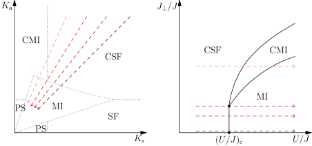
Figure 6: (Color online) A sketch of the trajectories of $K_{\mathrm{s}}$ and $K_{\mathrm{a}}$ for different values of $J_{\perp}/J$ (left panel), and schematic phase diagram as a function of the microscopic parameters (right panel). Each arrow in the left panel indicates the evolution of $K_{\mathrm{s}}$ and $K_{\mathrm{a}}$ as the interaction strength $U/J$ is increased. The rightmost arrow whose trajectory is described by $K_{\mathrm{s}}\simeq K_{\mathrm{a}}$ corresponds to the limit of decoupled chains $J_{\perp}/J\rightarrow 0$, and other arrows correspond to the gradual increase of $J_{\perp}/J$. Following the different trajectories in the generic phase diagram allows one to establish qualitatively the physical phase diagram displayed in the right panel.

III.1.3 Critical behavior

Closing the discussion on the ground-state phase diagram of the $\pi$ magnetic flux case at unity filling, we discuss the nature of the quantum critical behavior between the different phases.

Let us first consider the CSF-CMI transition. As in the effective theories, Eq. (50) for CSF, and Eq. (52) for CMI, the symmetric and antisymmetric sectors are decoupled in both regimes, and the transition is found to be characterized by the locking of the symmetric field $\varphi_{\mathrm{s}}$. Hence, focusing only on the symmetric sector in these two regimes, the phase transition from CSF to CMI is analogous to that of the sine-Gordon model. Thus the CSF-CMI transition is concluded to be of BKT transition nature, which is in agreement with the statement made in the numerical study of Ref. Dhar et al. (2012, 2013).

The nature of the CMI-MI transition is a more complicated issue, because the symmetric and antisymmetric sectors are coupled in the effective theory (54) of the MI regime. Comparing the effective theories $H^{(\mathrm{II})}_{\mathrm{eff}}$ and $H^{(\mathrm{IV})}_{\mathrm{eff}}$, two phenomena are found to occur at the transition from CMI to MI. One is the switch of the locked field in the antisymmetric sector, from $\theta_{\mathrm{a}}$ to $\varphi_{\mathrm{a}}$, and the other is the change of the locking value of the symmetric field $\varphi_{\mathrm{s}}$. In addition, the two-fold degeneracy caused by the fixed $\theta_{\mathrm{a}}$ in the CMI phase is found to change to a non-degenerate state in the MI phase. This change of the degeneracy means that the translation symmetry which is spontaneously broken in the CMI phase is restored in the MI phase. The nature is thus analogous to the $\mathbb{Z}_{2}$ Ising transition, which was also predicted for the CMI-MI transition for the frustrated bosonic ladder system Zaletel et al. (2014). The previous numerical studies Dhar et al. (2012, 2013) has pointed out the $\mathbb{Z}_{2}$ Ising criticality of the CMI-MI transition, and our field theoretical approach is thus consistent with this.

Finally we consider the direct phase transition between CSF and MI, shown in Fig. 6. Because of the coupling of the symmetric and antisymmetric sector in the MI phase, the analysis of this transition is not simple. Two simultaneous phenomena occur: the switch of the bound field from $\theta_{\mathrm{a}}$ to $\varphi_{\mathrm{a}}$ in the asymmetric sector and the locking of the field $\varphi_{\mathrm{s}}$ in the symmetric sector. This phase boundary is intriguing because two different symmetries are simultaneously involved: the continuous $O(2)$ symmetry associated with the SF and the $\mathbb{Z}_{2}$ symmetry associated with the breaking of translational invariance in the CSF phase. From usual considerations based on the Landau-Ginzburg-Wilson approach to critical phenomena, one may conclude that this phase transition is first-order. Indeed, according to Eq. (51), the local currents in the CSF phase do not depend on the interaction $U$, and the loop current is thus expected to discontinuously vanish when crossing the phase boundary from the CSF to MI phase. However, because the discussion which leads to the loop currents (51) is a kind of mean-field approach, a more in-depth discussion would be needed to obtain a crucial conclusion on the criticality. A more intriguing possibility on this criticality is that it might nonetheless be second-order, despite breaking simultaenously two unrelated symmetries Senthil et al. (2004a, b).

III.2 The ground state for small magnetic flux at unity filling

Next we discuss the phase diagram of the Bose-Hubbard ladder for a sufficiently small magnetic flux in which the bottom of the single particle spectrum shows a single energy minimum structure. In addition, we fix the filling at one particle per site. Then, setting $\bar{n}=1$, we can write the effective Hamiltonian (44) as

$$H_{\mathrm{eff}} =\frac{v}{2\pi}\int\!\!dx\,\left[K\left(\nabla\theta(x)\right)^{2}+\frac{1}{K}\left(\nabla\varphi(x)\right)^{2}\right]$$

$$\quad+g\int\!\!\frac{dx}{a}\,\cos\left(2\varphi(x)\right).$$ (57)

It has the same form as that of the single Bose-Hubbard chain. Thus a BKT transition is found when the Luttinger parameter as defined here reaches $K=2$. This transition is identical to the SF-Mott insulator transition Giamarchi (2004); Cazalilla et al. (2011). In the weakly interacting regime, the Luttinger parameter is larger than the critical value $K=2$, and the system is a gapless TL liquid, i.e. a one-dimensional SF. As the interaction is tuned to be larger, the Luttinger parameter becomes smaller, and the system becomes a MI for $K<2$. This behavior can be captured by the approximately estimated parameters (45): $K\propto U^{-1/2}$. The Luttinger parameter should be determined in terms of the interaction $U/J$ and the rung hopping $J_{\perp}/J$, but the corresponding critical value of these microscopic parameters can not be determined just from the field theoretical argument. Thus in this paper we do not discuss further quantitatively the ground-state phase diagram of the effective theory (57) in the microscopic parameter space.

Let us look at the ground-state physical properties of the gapless SF and MI phase predicted by the effective theory (57). As mentioned in Sec. II.3, the bosonized form of the current operators in Eq. (46) implies a non-zero constant current, which is displayed in Fig. 7. As given in the form, $\pm J\sin(\phi/2)$, this persistent current is induced by the magnetic flux, and is thus interpreted to be a Meissner current in the case of the ladder geometry. What is interesting is that the presence of this Meissner current is independent of the physics of the density fluctuation $\varphi$. On the other hand, even when the system is in the MI phase, in which $\varphi$ is locked by the cosine term, the Meissner current remains.

Figure 7: A pattern of Meissner currents appearing for a small magnetic flux. The strength of the Meissner current increases with the magnetic flux $\phi$. This current also remains even in the Mott insulator phase, but the chiral state is not gapless.

The physical reason of the presence of the Meissner current in the MI phase can be understood as follows. As well known, in the MI state, the phase of each bosons is completely disordered since the canonically conjugate density fluctuations are frozen. However, this statement does not forbid the lock of the relative phase between the bosons of the different component. Thus, in this MI case, each phase of the bosons on the upper and on the lower chain is disordered, but the relative phase between them is kept to be locked like that of the SF phase. Indeed, as mentioned in Ref.Orignac and Giamarchi (2001), the Meissner current is a consequence of the lock of the relative phase between the bosons on the upper and on the lower chain. A similar nature of the Meissner current in the fully gapped ground state was also pointed out in Ref. Petrescu and Le Hur (2013).

A question which naturally arises is what happens to the MI with Meissner currents in the limit of strong interactions. In our effective field theory approach (57), only two phases (SF and MI with Meissner currents) have been obtained. However, if we turn back to the original microscopic Hamiltonian, we do expect the current-carrying Mott state to be eventually unstable in favor of a conventional Mott state without currents. Indeed, in the weak-coupling effective field-theory, one first establishes the two-band structure of the non-interacting Hamiltonian and then turns on an interaction within the lowest band only (protected by a gap from the upper one). For a strong interaction, however, matrix elements of the interaction will couple the two bands, which may break the relative phase coherence between the two chains and lead to a conventional MI. This regime is away from the range of applicability of the effective field-theory approach.

From the above, we can describe the ground state of the unity-filling Bose-Hubbard ladder at a small magnetic flux as follows. In the weakly interacting regime, the system is a SF with Meissner currents, and the low-energy excitations carry chiral current, i.e., the directions of the carried currents on the upper and on the lower chain are opposite each other. On the other hand, in the strong interaction regime, the system is a MI in which the density fluctuations are completely suppressed, and there are no gapless excitations. However, this MI state still includes the Meissner current background. The transition between these two SF and MI phase is a BKT transition, as seen in a simple one-dimensional Bose-Hubbard chain at an integer filling. Furthermore, at strong interaction $U\gg J,J_{\perp}$, the MI with the Meissner current should turn into a conventional MI without currents. However, the transition and criticality between these two MI phases are not easily addressed within the present analysis.

IV Summary and perspectives

In this paper, we have discussed the Bose-Hubbard model with a uniform magnetic flux in ladder geometry. Discussing the small and large magnetic flux limits separately, we have constructed in each case the appropriate low-energy effective field theory by using bosonization techniques based on the nature of the single-particle spectrum. The key difference between the two cases is the number of lowest energy band minima. For a small magnetic flux, the bottom of the lowest band displays a single minimum. Increasing the magnetic flux beyond a critical value $\phi_{\mathrm{c}}$, this single minimum splits into two degenerate minima, which leads to a different structure of the low-energy field theory.

As an application of the derived effective field theories, we have discussed in detail the phases and physical properties of the system with one particle per site in the two cases of $\phi=\pi$ and small $\phi<\phi_{\mathrm{c}}$. For the $\pi$ magnetic flux, we have established the general ground-state phase diagram as a function of the Luttinger parameters characterizing the low-energy field theory. Several phases appear: a superfluid (SF), chiral superfluid (CSF), Mott insulator (MI), chiral Mott insulator (CMI), as well as a regime of density imbalance (DI). Furthermore, we have also discussed the mapping of this generic phase diagram in terms of the two microscopic parameters of the Bose-Hubbard model (the interaction strength $U/J$ and ratio of rung to in-chain hopping $J_{\perp}/J$). We have established that the CMI phase only occurs beyond a critical value of $J_{\perp}/J$, and to reveal the existence of a tricritical point at which the CSF, CMI and MI phases meet together. We also discussed the zero-temperature transitions and critical behavior separating these phases, and pointed out that the precise nature of the critical behavior for the direct transition between the CSF and MI phase is an interesting open issue to be addressed in future studies.

In the small magnetic flux case, we have clarified the possible ground states and their properties. The SF and MI states have been, respectively, found to appear at weak and strong interaction strength, with a BKT transition between them. We found that not only the SF state but also the MI state displays Meissner currents.

In a remarkable recent experiment Atala et al. (2014), Atala et al. realized a two-leg ladder optical lattice in which bosonic atoms are confined and subject to an artificial uniform magnetic field. The Meissner currents and vortex currents in the SF phase were successfully probed by using a site-resolved local current measurement Trotzky et al. (2012); Kessler and Marquardt (2013). These achievements should make it possible to investigate experimentally the various phases (SF, CSF, MI, CMI) discussed in the present work and to probe the Meissner currents and vortex structure. In addition, the tricritical point found in our study, and the nature of the CSF-MI transition could be put to the test in such experiments.

Appendix A Mean-field analysis to the long-wave-length effective Hamiltonian

Here we present the mean-field approach to determine the chemical potential in the effective Hamiltonian given by the long-wave-length approximation.

A.1 Large magnetic flux case

First let us see the case of the large magnetic flux, in which the single-particle spectrum forms the double minima in the lower energy band. Based on the Hamiltonian (18) and (19) derived by the long-wave-length approximation the mean-field energy per site, in which the quantum fluctuations are ignored, is assumed to be

$$E_{\mathrm{MF}} =-\frac{1}{2}\left(\mu+E_{0}+\frac{U}{2}-UV_{+}^{2}V_{-}^{2}\right)\left(\tilde{n}_{+}+\tilde{n}_{-}\right)$$

$$\quad+\frac{U\left(1+2V_{+}^{2}V_{-}^{2}\right)}{8}\left(\tilde{n}_{+}+\tilde{n}_{-}\right)^{2}$$

$$\quad+\frac{U\left(1-6V_{+}^{2}V_{-}^{2}\right)}{8}\left(\tilde{n}_{+}-\tilde{n}_{-}\right)^{2},$$ (58)

where $\tilde{n}_{\pm}=\langle{\tilde{n}_{\pm,j}}\rangle$. From the mean-field energy, the mean-field equations for the density of the bosons populating at each band minima are derived by $\partial{E_{\mathrm{MF}}}/{\partial{\tilde{n}_{\pm}}}=0$, and lead to the mean-field solution $\bar{n}=\tilde{n}_{+}=\tilde{n}_{-}$ with

$$\mu=-E_{0}+U\left(\bar{n}-\frac{1}{2}\right)+V^{2}_{+}V^{2}_{-}U\left(2\bar{n}+1\right),$$ (59)

which determines the chemical potential for the given density $\tilde{n}_{\pm}$. The obtained mean-field density $\bar{n}$ can be associated with those of the chains, $\bar{n}_{p}=\langle{n_{j,p}}\rangle$ ($p=1,2$), in the original representation. The approximated form of the densities (17) leads to

$$\bar{n}_{1}=V^{2}_{-}\tilde{n}_{+}+V^{2}_{+}\tilde{n}_{-},$$

$$\bar{n}_{2}=V^{2}_{+}\tilde{n}_{+}+V^{2}_{-}\tilde{n}_{+},$$ (60)

and $\bar{n}_{1}=\bar{n}_{2}=\bar{n}$ is immediately concluded since $\tilde{n}_{\pm}=\bar{n}$ and $V^{2}_{+}+V^{2}_{-}=1$.

In addition, the stability of the mean-field solution is confirmed by the positive definiteness of Hessian matrix $H_{\alpha,\beta}=\partial^{2}{E_{\mathrm{MF}}}/\partial{\tilde{n}_{\alpha}}\partial{\tilde{n}_{\beta}}>0$ ($\alpha,\beta=\pm$). From the straightforward calculation of the eigenvalues of the Hessian matrix, the condition of the stable mean-field solution is found to be reduced to

$$\left(\frac{J_{\perp}}{2J}\right)^{2}<\frac{2\sin^{4}\left(\phi/2\right)}{3-2\sin^{2}\left(\phi/2\right)}.$$ (61)

This condition needs the smaller rung hopping as $\phi$ decreases. For example, for the largest magnetic flux case $\phi=\pi$, it leads to $J_{\perp}^{2}<8J^{2}$, and for the less flux $\phi=\pi/2$, $J_{\perp}^{2}<J^{2}$ is needed.

A.2 Small magnetic flux case

Next we consider the small magnetic flux case, in which the low-energy single-particle spectrum shows a single minimum in the bottom of the lower energy band. Neglecting the quantum fluctuations in the approximated long-wave-length Hamiltonian (42), the mean-field energy is given by

$$E_{\mathrm{MF}}=-\frac{1}{2}\left(\mu+E_{0}+\frac{U}{2}\right)\tilde{n}+\frac{U}{8}\tilde{n}^{2},$$ (62)

where $\tilde{n}=\langle{\tilde{n}_{j}}\rangle$ in Eq. (42). Thus the mean-field solution is given by $\partial{E_{\mathrm{MF}}}/\partial{\tilde{n}}=0$, which is

$$\mu=-E_{0}+\frac{U}{2}\left(\tilde{n}-1\right).$$ (63)

In addition, from the second-order derivative of the mean-field energy, the above mean-field solution is immediately found to be stable. The mean density on the chains is balanced as in Eq. (41), i.e., $\langle{n_{j,1}}\rangle=\langle{n_{j,2}}\rangle=\tilde{n}/2$. Thus, supposing the balanced mean density on the chains to be $\bar{n}$, this density is controlled by the chemical potential as

$$\bar{n}=\frac{1}{U}\left(\mu+E_{0}+\frac{U}{2}\right).$$ (64)

References

- Dalibard et al. (2011) J. Dalibard, F. Gerbier, G. Juzeliūnas, and P. Öhberg, Rev. Mod. Phys. 83, 1523 (2011).
- Berry (1984) M. V. Berry, Proceedings of the Royal Society of London. A. Mathematical and Physical Sciences 392, 45 (1984).
- Dum and Olshanii (1996) R. Dum and M. Olshanii, Phys. Rev. Lett. 76, 1788 (1996).
- Lin et al. (2009) Y.-J. Lin, R. L. Compton, K. Jimenez-Garcia, J. V. Porto, and I. B. Spielman, Nature 462, 628 (2009).
- Lin et al. (2011) Y.-J. Lin, K. Jimenez-Garcia, and I. B. Spielman, Nature 471, 83 (2011).
- Wang et al. (2012) P. Wang, Z.-Q. Yu, Z. Fu, J. Miao, L. Huang, S. Chai, H. Zhai, and J. Zhang, Phys. Rev. Lett. 109, 095301 (2012).
- Cheuk et al. (2012) L. W. Cheuk, A. T. Sommer, Z. Hadzibabic, T. Yefsah, W. S. Bakr, and M. W. Zwierlein, Phys. Rev. Lett. 109, 095302 (2012).
- Beeler et al. (2013) M. C. Beeler, R. A. Williams, K. Jimenez-Garcia, L. J. LeBlanc, A. R. Perry, and I. B. Spielman, Nature 498, 201 (2013), letter.
- Jaksch and Zoller (2003) D. Jaksch and P. Zoller, New Journal of Physics 5, 56 (2003).
- Sørensen et al. (2005) A. S. Sørensen, E. Demler, and M. D. Lukin, Phys. Rev. Lett. 94, 086803 (2005).
- Mueller (2004) E. J. Mueller, Phys. Rev. A 70, 041603 (2004).
- Lim et al. (2008) L.-K. Lim, C. M. Smith, and A. Hemmerich, Phys. Rev. Lett. 100, 130402 (2008).
- Lim et al. (2010) L.-K. Lim, A. Hemmerich, and C. M. Smith, Phys. Rev. A 81, 023404 (2010).
- Aidelsburger et al. (2011) M. Aidelsburger, M. Atala, S. Nascimbène, S. Trotzky, Y.-A. Chen, and I. Bloch, Phys. Rev. Lett. 107, 255301 (2011).
- Aidelsburger et al. (2013a) M. Aidelsburger, M. Atala, S. Nascimbène, S. Trotzky, Y.-A. Chen, and I. Bloch, Applied Physics B 113, 1 (2013a).
- Miyake et al. (2013) H. Miyake, G. A. Siviloglou, C. J. Kennedy, W. C. Burton, and W. Ketterle, Phys. Rev. Lett. 111, 185302 (2013).
- Kennedy et al. (2013) C. J. Kennedy, G. A. Siviloglou, H. Miyake, W. C. Burton, and W. Ketterle, Phys. Rev. Lett. 111, 225301 (2013).
- Aidelsburger et al. (2013b) M. Aidelsburger, M. Atala, M. Lohse, J. T. Barreiro, B. Paredes, and I. Bloch, Phys. Rev. Lett. 111, 185301 (2013b).
- Jiménez-García et al. (2012) K. Jiménez-García, L. J. LeBlanc, R. A. Williams, M. C. Beeler, A. R. Perry, and I. B. Spielman, Phys. Rev. Lett. 108, 225303 (2012).
- Struck et al. (2012) J. Struck, C. Ölschläger, M. Weinberg, P. Hauke, J. Simonet, A. Eckardt, M. Lewenstein, K. Sengstock, and P. Windpassinger, Phys. Rev. Lett. 108, 225304 (2012).
- Simonet, J. et al. (2013) Simonet, J., Struck, J., Weinberg, M., Ölschläger, C., Hauke, P., Eckardt, A., Lewenstein, M., Sengstock, K., and Windpassinger, P., EPJ Web of Conferences 57, 01004 (2013).
- Struck et al. (2013) J. Struck, M. Weinberg, C. Olschlager, P. Windpassinger, J. Simonet, K. Sengstock, R. Hoppner, P. Hauke, A. Eckardt, M. Lewenstein, and L. Mathey, Nat Phys 9, 738 (2013), article.
- Carr et al. (2006) S. T. Carr, B. N. Narozhny, and A. A. Nersesyan, Phys. Rev. B 73, 195114 (2006).
- Jaefari and Fradkin (2012) A. Jaefari and E. Fradkin, Phys. Rev. B 85, 035104 (2012).
- Roux et al. (2007) G. Roux, E. Orignac, S. R. White, and D. Poilblanc, Phys. Rev. B 76, 195105 (2007).
- Schollwöck et al. (2003) U. Schollwöck, S. Chakravarty, J. O. Fjærestad, J. B. Marston, and M. Troyer, Phys. Rev. Lett. 90, 186401 (2003).
- Denniston and Tang (1995) C. Denniston and C. Tang, Phys. Rev. Lett. 75, 3930 (1995).
- Kardar (1986) M. Kardar, Phys. Rev. B 33, 3125 (1986).
- Granato (1990) E. Granato, Phys. Rev. B 42, 4797 (1990).
- Nishiyama (2000) Y. Nishiyama, The European Physical Journal B - Condensed Matter and Complex Systems 17, 295 (2000).
- Orignac and Giamarchi (2001) E. Orignac and T. Giamarchi, Phys. Rev. B 64, 144515 (2001).
- Petrescu and Le Hur (2013) A. Petrescu and K. Le Hur, Phys. Rev. Lett. 111, 150601 (2013).
- Dhar et al. (2013) A. Dhar, T. Mishra, M. Maji, R. V. Pai, S. Mukerjee, and A. Paramekanti, Phys. Rev. B 87, 174501 (2013).
- Dhar et al. (2012) A. Dhar, M. Maji, T. Mishra, R. V. Pai, S. Mukerjee, and A. Paramekanti, Phys. Rev. A 85, 041602 (2012).
- Crépin et al. (2011) F. m. c. Crépin, N. Laflorencie, G. Roux, and P. Simon, Phys. Rev. B 84, 054517 (2011).
- Tovmasyan et al. (2013) M. Tovmasyan, E. P. L. van Nieuwenburg, and S. D. Huber, Phys. Rev. B 88, 220510 (2013).
- Atala et al. (2014) M. Atala, M. Aidelsburger, M. Lohse, J. T. Barreiro, B. Paredes, and I. Bloch, ArXiv e-prints (2014), arXiv:1402.0819 [cond-mat.quant-gas] .
- Donohue and Giamarchi (2001) P. Donohue and T. Giamarchi, Phys. Rev. B 63, 180508 (2001).
- Hügel and Paredes (2014) D. Hügel and B. Paredes, Phys. Rev. A 89, 023619 (2014).
- Oshikawa (2010) M. Oshikawa, ArXiv e-prints (2010), arXiv:1007.3739 [cond-mat.stat-mech] .
- Oshikawa et al. (2006) M. Oshikawa, C. Chamon, and I. Affleck, Journal of Statistical Mechanics: Theory and Experiment 2006, P02008 (2006).
- Wong and Affleck (1994) E. Wong and I. Affleck, Nuclear Physics B 417, 403 (1994).
- Giamarchi (2004) T. Giamarchi, Quantum Physics in One Dimension (Oxford University Press, Oxford, 2004).
- Berezinskii (1971) V. L. Berezinskii, Journal of Experimental and Theoretical Physics 32, 493 (1971).
- Berezinskii (1972) V. L. Berezinskii, Journal of Experimental and Theoretical Physics 34, 610 (1972).
- Kosterlitz and Thouless (1973) J. M. Kosterlitz and D. J. Thouless, Journal of Physics C: Solid State Physics 6, 1181 (1973).
- Note (1) Note that the choice of gauge (5) preserves translational symmetry of the Hamiltonian. If we take another choice of gauge, and , the translation symmetry preserved in the choice of gauge (5) is explicitly broken.
- Cazalilla (2004) M. A. Cazalilla, Journal of Physics B: Atomic, Molecular and Optical Physics 37, S1 (2004).
- Zaletel et al. (2014) M. P. Zaletel, S. A. Parameswaran, A. Rüegg, and E. Altman, Phys. Rev. B 89, 155142 (2014).
- Senthil et al. (2004a) T. Senthil, A. Vishwanath, L. Balents, S. Sachdev, and M. P. A. Fisher, Science 303, 1490 (2004a), http://www.sciencemag.org/content/303/5663/1490.full.pdf .
- Senthil et al. (2004b) T. Senthil, L. Balents, S. Sachdev, A. Vishwanath, and M. P. A. Fisher, Phys. Rev. B 70, 144407 (2004b).
- Cazalilla et al. (2011) M. A. Cazalilla, R. Citro, T. Giamarchi, E. Orignac, and M. Rigol, Rev. Mod. Phys. 83, 1405 (2011).
- Trotzky et al. (2012) S. Trotzky, Y.-A. Chen, A. Flesch, I. P. McCulloch, U. Schollwock, J. Eisert, and I. Bloch, Nat Phys 8, 325 (2012).
- Kessler and Marquardt (2013) S. Kessler and F. Marquardt, ArXiv e-prints (2013), arXiv:1309.3890 [cond-mat.quant-gas] .