Positronium resonance contribution to the electron $g-2$

Abstract

Recently a few authors pointed out that the positroniums give rise to an extra contribution to the electron $g-2$ which is independent of the perturbative calculation up to $O(\alpha^{5})$ and has the same magnitude as the $O(\alpha^{5})$ perturbative effect. Here, we scrutinize how the positronium resonances contribute to the electron $g-2$ through the vacuum polarization function, and conclude that there is no additional sizable $O(\alpha^{5})$ contribution from the positronium resonances to the electron $g-2$.

I Introduction

Recently, Ref. Mishima:2013ama pointed out that the positroniums in the vector channel give an additional contribution to the electron $g-2$, $a_{e}$, which cannot be captured by the perturbative analysis up to $O(\alpha^{5})$ Aoyama:2012wj . Subsequently, Ref. Fael:2014nha checked the calculation in Ref. Mishima:2013ama and presented an updated value for such a contribution. They concluded that the correction is independent of the perturbative contribution and has the same order of magnitude as the $O(\alpha^{5})$ perturbative contribution and thus affects to the comparison of the experiment and the theory of $a_{e}$.

The assertion in Refs. Mishima:2013ama ; Fael:2014nha seems to be gradually attaining the consensus in the community of particle phenomenology. During the preparation of this article, the two papers Melnikov:2014lwa ; Eides:2014swa presented a negative conclusion on the results in Refs. Mishima:2013ama ; Fael:2014nha . In such a circumstance, this article attempts to scrutinize the current issue from the basic of the quantum field theory. The consideration in full order QED in Sec. II shows that Refs. Mishima:2013ama ; Fael:2014nha do not dealt with the contribution of the positronium resonances. The proper identification of such a contribution immediately shows that there is no contribution to $a_{e}$ from the positronium resonances with the size found in Refs. Mishima:2013ama ; Fael:2014nha .

In Sec. II, we start with summarizing the question to be addressed here and present the answer to it. Section III discusses the connection of this paper with those of the precedence works Mishima:2013ama ; Fael:2014nha ; Melnikov:2014lwa ; Eides:2014swa . It turns out that the analysis perspective itself, which provides a more convincing approach to the question, is quite different from that in Refs. Mishima:2013ama ; Fael:2014nha ; Melnikov:2014lwa ; Eides:2014swa .

II Positronium contribution

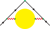
Figure 1: Contribution to the electron $g-2$ from the vacuum polarization function induced by QED (the blob part). The black and wavy red lines denote the propagation of electron and photon, respectively.

Following Ref. Mishima:2013ama , we restrict our attention to the type of the QED contribution induced through the vacuum polarization to the electron $g-2$ as shown in Fig. 1.

In order to disentangle the confusion, we first marshal the question itself to be addressed here : How large is the contribution from the positroniums in the vector channel to the electron $g-2$ through Fig. 1.

To this end, we start with reconsidering full-order QED contribution to the two-point function of the electromagnetic current $j_{\mu}\equiv-e\,\overline{\psi}\gamma_{\mu}\psi$ in the QED with the electron only, which suffices for the succeeding discussion

$$\int d^{4}x\,e^{{\rm i}q\cdot x}\,\left<0\right|Tj_{\mu}(x)j^{\nu}(0)\left|0\right>_{\rm 1PI}={\rm i}\left(\delta_{\mu}^{\ \nu}q^{2}-q_{\mu}q^{\nu}\right)\Pi(q^{2})\,.$$ (1)

The renormalized function will be obtained by $\Pi_{\rm R}(q^{2})=\Pi(q^{2})-\Pi(0)$.

Since QED does not have any nontrivial classical gauge configurations such as instantons, we can identify which set of Feynman diagrams, e.g. an infinite series of ladder diagrams, is associated with the quantum dynamics relevant to the phenomenon of one’s interest.

It is worthwhile to recall some basic features of the state space and $\Pi(q^{2})$. The physical space of QED is spanned by stable one-particle states and multi-particle states composed of them. Since confinement does not occur and no stable bound state exists in QED, the only one-particle states are photon, electron and positron. Every multi-particle state consists of photon(s) and electron(s).

The vacuum polarization function $\Pi(q^{2})$ defined in Eq. (1) is analytic on the surface obtained from two complex planes by braiding on the branch cuts. Each of the branch cuts is associated with a multi-particle state $\left|\Psi;\,\left\{{\bf q}_{j},\,\lambda_{j}\right\}_{j}\right>$ ($\lambda_{j}$ denotes the polarization.) that couples non-trivially to the electromagnetic current $j_{\mu}$; $\left<0\right|j_{\mu}(0)\left|\Psi;\,\left\{{\bf q}_{j},\,\lambda_{j}\right\}_{j}\right>\neq 0$. The examples of such multi-particle states are multi-photons, $3\gamma$, $5\gamma$, or $e^{-}e^{+}$, $e^{-}e^{+}\gamma$, etc. The kinematics involved in the matrix element, say, $\left<0\right|j_{\mu}(0)\left|3\gamma;\,\left\{{\bf q}_{j},\,\lambda_{j}\right\}_{j=1,2,3}\right>$ can be found in Ref. Costantini:1971cj . With this analytic structure of $\Pi(q^{2})$ in our mind, we derive the dispersion relation for $\Pi_{\rm R}(q^{2})/q^{2}$ after introducing the infrared regulator so that the branch cuts of multi-photons start from infinitesimally small constant $s_{0}>0$

$$\frac{\Pi_{\rm R}(q^{2}+{\rm i}\epsilon)}{q^{2}+{\rm i}\,\epsilon}=-\frac{1}{\pi}\int_{0+}^{\infty}\frac{ds}{s}\,\frac{{\rm Im}\,\Pi_{\rm R}(s+{\rm i}\,0)}{q^{2}-s+{\rm i}\epsilon}\,.$$ (2)

This together with Eq. (1) immediately yields the expression for the contribution to $a_{e}$ of the type in FIG. 1 as a superposition of the contribution $a_{e}(s)$ from the vector boson with mass squared $s$ weighted by ${\rm Im}\,\Pi_{\rm R}(s+{\rm i}\,0)$

$$a_{e}[{\rm vp}]=\int_{0+}^{\infty}\frac{ds}{s}\,{\rm Im}\,\Pi_{\rm R}(s+{\rm i}\,0)\,a_{e}(s)\,.$$ (3)

In fact, the branch cuts associated with the multi-photons are overlooked in FIG. 3 of Ref. Mishima:2013ama . Instead, $\Pi(q^{2})$ is supposed to have complex poles. However, complex poles are just the concepts that are often introduced temporarily in particle phenomenology for the purpose to calculate the total decay width and make comparison with the experiments. The imaginary part of a complex pole, the decay width, depends upon one’s definition. The requirement of the gauge independence, for instance, may motivate to choose a more favorable one Sirlin:1991rt . Theoretically, the unitarity is assured only if $\Pi(q^{2})$ can receive nontrivial contribution from the states $\left|\Psi;\,\left\{{\bf q}_{j},\,\lambda_{j}\right\}_{j}\right>$ such that $\left<0\right|j_{\mu}(0)\left|\Psi;\,\left\{{\bf q}_{j},\,\lambda_{j}\right\}_{j}\right>\neq 0$, which results in producing the branch cuts of $\Pi(q^{2})$.

Figure 2: A typical positronium contribution to the vacuum polarization function. The blob part denotes the one-particle irreducible correlation function of four electromagnetic currents.

Now, Eq. (3) together with the above remark on the analytic property of $\Pi_{\rm R}(q^{2})$ immediately allows to identify which type of diagrams contains the positronium contribution. The ortho-positronium contribution is associated with ${\rm Im}\,\Pi_{\rm R}(s)$ originating from $(2n+3)\gamma$ states ($n=0,\,1,\,2,\cdots$). This is because the component involved in the state $j_{\mu}(0)\left|0\right>$ that can be considered as the positronium ground state, say, should be concentrated in the region centered at $\sqrt{s}\simeq 2m_{e}-\alpha^{2}m_{e}/4$ with the narrow width $\propto\alpha^{6}m_{e}$ so that its overlap with each multi-state containing $e^{-}e^{+}$ is vanishing small. Therefore, the physical ortho-positronium resonance contribution comes from, say, the diagram in FIG. 1, but with the vacuum polarization part replaced by a particular form shown in FIG. 2, which is distinctly different than that dealt with in Refs. Mishima:2013ama ; Fael:2014nha and essentially that in Refs. Melnikov:2014lwa ; Eides:2014swa . Such diagrams at the leading-order will be $O(\alpha^{7})$ if at least one photon must be exchanged in each of the two light-by-light scattering amplitudes in FIG. 2 to form a positronium. The smallness of such a contribution will be speculated from the result Aoyama:2008gy for the $O(\alpha^{5})$ contribution to $a_{e}$ caused by the diagrams of the type in FIG. 2 with the one-loop light-by-light scattering subdiagrams, which belong to Set I(j) according to the classification scheme of $O(\alpha^{5})$ diagrams Aoyama:2005kf ; Kinoshita:2005sm

$$a_{e}[{\rm I(j)},e\ {\rm only}]=0.000\ 3950\ (87)\left(\frac{\alpha}{\pi}\right)^{5}\,.$$ (4)

This is quite smaller than the dominant tenth-order contribution which is found to have magnitude $O(1)\times(\alpha/\pi)^{5}$ Aoyama:2012wj . The resonance contribution starting at $O(\alpha^{7})$ will be further suppressed by the factor $\left(\alpha/\pi\right)^{2}$.

In this paper, we see how the physical positronium resonance contributes to the electron $g-2$ through the diagram in FIG. 2. Needless to say, there is no systematic way to single out the resonance contribution by separating it from the continuum contribution. Properly speaking, what is done above is to correctly identify a set of the diagrams which contains the contribution of positronium resonances in the vector channel.

III Conclusion and discussion

The plain consideration in Sec. II enabled us to correctly identify a set of diagrams that contain the positronium resonance contribution, and leads the conclusion that there is no additional nonperturbative correction to the electron $g-2$ of the same size as the perturbative correction of $O(\alpha^{5})$ as was first pointed out in Ref. Mishima:2013ama . Here, we discuss the connection of our founding with the precedence works concerning with the current issue.

Obviously, the difference of this work from Refs. Mishima:2013ama ; Fael:2014nha ; Melnikov:2014lwa ; Eides:2014swa stems from the fact that we never neglect the instability of the positroniums and deal with the proper space of states in QED. The question to be addressed in this article is defined at the beginning of Sec. II, and we obtain a definite answer to it. In contrast, the other works seems to cast the following question by neglecting the unstable character of positroniums: Is the QED dynamics which are mainly concerned with the formation of positroniums give rise to an additional nonperturbative contribution to the electron $g-2$ ?

Instead of chasing the details of the discussions in Refs. Mishima:2013ama ; Fael:2014nha ; Melnikov:2014lwa ; Eides:2014swa , we discuss the following points in the rest of the paper:

• On one hand, one focuses on some coulombic dynamics nonperturbatively. On the other hand, one wishes to forbid the decay of the bound state, which cannot be realized just from the perturbative order counting. We examine theoretically what concrete approximation reconciles these seemingly contradictory situations.

• There is no local field theory that reproduces only the approximation to the two-point function, i.e. the connected diagram contribution. It is thus inevitable to deal with another types of contribution which unstabilize positroniums, and to examine the current issue by working with the state space as described in Sec. II.

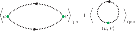
Figure 3: Connected diagram contribution to the two point function of the electromagnetic currents in lattice QED. An arrowed dotted line represents the inverse of the electron Dirac operator, $D[A]^{-1}(x,\,y)$. $\left<\mathcal{Q}\right>_{\rm QED}$ denotes the vacuum expectation value of the quantity $\mathcal{Q}$ in QED. The second term contributes only if the positions of the two current operators coincide with each other.

We adopt the lattice regulariation for QED just because the terminology in the framework of the lattice field theory is used in the following discussion. Figure 3 corresponds to the (gauge-invariant) nonperturbative approximation to the vacuum polarization function (1) taken in Refs. Mishima:2013ama ; Fael:2014nha ; Melnikov:2014lwa ; Eides:2014swa . Each arrowed dashed line in that figure is not the fermion propagator in the perturbation theory, but the inverse of the Dirac operator of the electron, $D[A]^{-1}(x,\,y)$, under a given gauge potential $A$. The symbol $\left<\mathcal{Q}[A]\right>_{\rm QED}$ denotes the vacuum expectation value (VEV) of a quantity $\mathcal{Q}[A]$ that depends only on the gauge potential in QED

$$\left<\mathcal{Q}[A]\right>_{\rm QED}= \,\frac{1}{Z_{\rm QED}}\int d\psi\,d\overline{\psi}\,dA\,\exp\left({\rm i}S_{\rm QED}\left[A,\,\psi,\,\overline{\psi}\right]\right)\mathcal{Q}[A]$$

$$= \,\frac{1}{Z_{\rm QED}}\int dA\,\exp\left({\rm i}S_{\rm G}[A]\right){\rm det}\left(-D[A]\right)\,\mathcal{Q}[A]\,,$$

$$S_{\rm QED}\left[A,\,\psi,\,\overline{\psi}\right]= S_{\rm G}[A]+a^{4}\sum_{x}\overline{\psi}(x)({\rm i}D[A]\psi)(x)\,,$$

$$S_{\rm G}[A]= \,a^{4}\sum_{x}\left\{-\frac{1}{4}\,F_{\mu\nu}(x)\,F^{\mu\nu}(x)+\frac{1}{2\lambda}\left(\partial\kern-0.5pt\smash{\raise 4.5pt\hbox{$\ast$}}\kern-5.0pt_{\mu}A^{\mu}\right)^{2}\right\}\,,$$

$$Z_{\rm QED}= \int d\psi\,d\overline{\psi}\,dA\,\exp\left({\rm i}S_{\rm QED}\left[A,\,\psi,\,\overline{\psi}\right]\right)\,,$$ (5)

where“$a$” denotes the lattice spacing, $F_{\mu\nu}(x)$ in the noncompact formulation of the lattice QED takes the familiar form $F_{\mu\nu}(x)=\partial_{\mu}A_{\nu}(x)-\partial_{\nu}A_{\mu}(x)$ but with the forward difference $a\,{\partial_{\mu}}f(x)\equiv f(x+a\widehat{\mu})-f(x)$, and $\partial\kern-0.5pt\smash{\raise 4.5pt\hbox{$\ast$}}\kern-5.0pt_{\mu}$ denotes the backward difference operator; $a\,\partial\kern-0.5pt\smash{\raise 4.5pt\hbox{$\ast$}}\kern-5.0pt_{\mu}f(x)\equiv f(x)-f(x-a\widehat{\mu})$. The tadpole diagram in FIG. 3 appears because $D[A]$ involves the Wilson line, $e^{-{\rm i}e\,aA_{\mu}(x)}$, which parallel-transports back the variable at $x+a\widehat{\mu}$ to $x$.

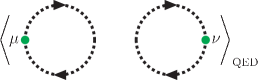
Figure 4: Disconnected diagram contribution to the correlation function of two electromagnetic currents. The diagram in FIG. 2 appears as a part of this type of diagrams.

Noting that the VEV of the operator $O\left[\psi,\,\overline{\psi},\,A\right]$ depending on the electron fields can be converted to that of $\widehat{O}[A]$ defined by

$$\widehat{O}[A]\equiv\left[O\left[\frac{1}{a^{4}}\frac{\partial^{L}}{{\rm i}\partial\overline{\eta}},\,\frac{1}{a^{4}}\frac{\partial^{R}}{{\rm i}\partial\eta},\,A\right]\exp\left(a^{4}\sum_{x}a^{4}\sum_{y}{\rm i}\overline{\eta}(x)\,D[A]^{-1}(x,\,y)\,{\rm i}\eta(y)\right)\right]_{\eta,\,\overline{\eta}\rightarrow 0}\,,$$ (6)

with the left (right) derivative $\partial^{L}/\partial\overline{\eta}(x)$ ($\partial^{R}/\partial\eta(y)$), the total contribution to the full correlation function of two electromagnetic currents

$$\int d^{4}x\,e^{{\rm i}q\cdot x}\,\left<0\right|Tj_{\mu}(x)j^{\nu}(0)\left|0\right>={\rm i}\left(\delta_{\mu}^{\ \nu}q^{2}-q_{\mu}q^{\nu}\right)J(q^{2})\,,$$ (7)

is found to be given by the sum of the connected diagram in FIG. 3 and the disconnected diagram shown in FIG. 4, which also contains the contribution of the one-particle reducible diagrams. A simple diagrammatic consideration enables to express $J(q^{2})$ in term of $\Pi(q^{2})$

$$J(q^{2})=\frac{\Pi(q^{2})}{1+\Pi(q^{2})}\,.$$ (8)

We recall that the disconnected diagram contains the diagrams responsible to the decay of the positroniums.

The simulation of the connected diagram in FIG. 3 will allow to measure the masses of the pseudo-bound states in the vector channel that are absolutely stable. However, the connected diagram contains, say, the ladder-type photon exchange only in the “$t$-channel”, where the“$s$-channel” is taken to be in the direction of the injected momentum in FIG. 3. If we cut the subdiagrams with four external fermion lines out of a perturbative diagram of the type in FIG. 3 and embed it again into the rest of the original after rotating it by $90$ degrees in a clockwise direction, we will obtain a diagram of the type in FIG. 4. This indicates that there is no local Lagrangian density that reproduces the contribution from the connected diagram and no contribution from disconnected diagram.

The situation should be contrasted with the case in which the decay process caused by the weak interaction is neglected. Then, there exists a local field theory that describes the system with the weak interaction switched off , and we can construct the state space at the zeroth-order of the approximation. A more concrete and familiar example is the description of hadron physics where the zeroth-order is approximated by the world with QCD only and the corrections due to QED and the dynamics of weak interactions are managed perturbatively. If no local field theory describing the zeroth-order approximation exists, we cannot proceed with the calculation of $a_{e}$ with use of the dispersion relation as Eq. (3) which relies on the analytic property of $\Pi(q^{2})$, the existence of the state space and unitarity. Hence, we have to tackle with the current issue using the state space described as in Sec. II and Eq. (3). The connected diagram in FIG. 3 gives a significant contribution to the electron $g-2$. Eq. (3) implies that such a contribution comes from the intermediate states of $e^{-}e^{+}$, $e^{-}e^{+}\gamma$, etc. and can be calculated by means of perturbation.

- (1) G. Mishima, Bound State Effect on the Electron , arXiv:1311.7109 [hep-ph].
- (2) T. Aoyama, M. Hayakawa, T. Kinoshita and M. Nio, Tenth-Order QED Contribution to the Electron and an Improved Value of the Fine Structure Constant, Phys. Rev. Lett. 109, 111807 (2012) [arXiv:1205.5368 [hep-ph]].
- (3) M. Fael and M. Passera, On the positronium contribution to the electron , arXiv:1402.1575 [hep-ph].
- (4) K. Melnikov, A. Vainshtein and M. Voloshin, Remarks on the effect of bound states and threshold in , arXiv:1402.5690 [hep-ph].
- (5) M. I. Eides, On Some Recent Ideas on the Proton Radius Puzzle and Lepton Anomalous Magnetic Moments, arXiv:1402.5860 [hep-ph].
- (6) V. Costantini, B. De Tollis and G. Pistoni, Nonlinear effects in quantum electrodynamics, Nuovo Cim. A 2, 733 (1971).
- (7) A. Sirlin, Observations concerning mass renormalization in the electroweak theory, Phys. Lett. B 267, 240 (1991).
- (8) T. Aoyama, M. Hayakawa, T. Kinoshita and M. Nio, Automated calculation scheme for contributions of QED to lepton : Generating renormalized amplitudes for diagrams without lepton loops, Nucl. Phys. B 740, 138 (2006) [hep-ph/0512288].
- (9) T. Kinoshita and M. Nio, The Tenth-order QED contribution to the lepton : Evaluation of dominant terms of muon , Phys. Rev. D 73, 053007 (2006) [hep-ph/0512330].
- (10) T. Aoyama, M. Hayakawa, T. Kinoshita, M. Nio and N. Watanabe, Eighth-Order Vacuum-Polarization Function Formed by Two Light-by-Light-Scattering Diagrams and its Contribution to the Tenth-Order Electron , Phys. Rev. D 78, 053005 (2008) [arXiv:0806.3390 [hep-ph]].
- (11) G. M. de Divitiis et al., Leading isospin breaking effects on the lattice, Phys. Rev. D 87, 114505 (2013) [arXiv:1303.4896 [hep-lat]].