The BANANA project. V. Misaligned and precessing stellar rotation axes in CV Velorum.^⋆

Abstract

As part of the BANANA project (Binaries Are Not Always Neatly Aligned), we have found that the eclipsing binary CV Velorum has misaligned rotation axes. Based on our analysis of the Rossiter-McLaughlin effect, we find sky-projected spin-orbit angles of $\beta_{\rm p}=-52\pm 6^{\circ}$ and $\beta_{\rm s}=3\pm 7^{\circ}$ for the primary and secondary stars (B2.5V $+$ B2.5V, $P=6.9$ d). We combine this information with several measurements of changing projected stellar rotation speeds ($v\sin i_{\star}$) over the last $30$ years, leading to a model in which the primary star’s obliquity is $\approx 65^{\circ}$, and its spin axis precesses around the total angular momentum vector with a period of about $140$ years. The geometry of the secondary star is less clear, although a significant obliquity is also implicated by the observed time variations in the $v\sin i_{\star}$. By integrating the secular tidal evolution equations backward in time, we find that the system could have evolved from a state of even stronger misalignment similar to DI  Herculis, a younger but otherwise comparable binary.

1. Introduction

Stellar obliquities (spin-orbit angles) have been measured in only a handful of binary stars. (see Albrecht et al., 2011, for a compilation). The case of DI Herculis, in which both stars have large obliquities (Albrecht et al., 2009), has taught us that it is risky to assume that the orbital and spin axes are aligned. For one thing, misalignment can influence the observed stellar parameters; for example, the rotation axes may precess, producing time variations in the sky-projected rotation speeds (Albrecht et al., 2009; Reisenberger & Guinan, 1989). Precession would also produce small changes in the orbital inclination, and therefore changes in any eclipse signals. Misalignment also influences the rate of apsidal precession, as predicted by Shakura (1985) for the case of DI Her and confirmed by Albrecht et al. (2009), and as is suspected to be the case for AS Cam (Pavlovski et al., 2011).

Furthermore, measurements of obliquities should be helpful in constraining the formation and evolution of binary systems. Larger obliquities might indicate that a third star on a wide, inclined orbit gave rise to Kozai cycles in the close pair during which the close pair’s orbital eccentricity and inclination oscillate (Mazeh & Shaham, 1979; Eggleton & Kiseleva-Eggleton, 2001; Fabrycky & Tremaine, 2007; Naoz et al., 2013). A third body on an inclined orbit might also cause orbital precession of the inner orbit around the total angular momentum, again creating large opening angles between the stellar rotation and the orbit of the close pair (Eggleton & Kiseleva-Eggleton, 2001). There are also other mechanisms which can lead to apparent misalignments. For example Rogers et al. (2012, 2013) suggest that for stars with an outer radiative layer, large angles between the convective core and the outer layer may be created by internal gravity waves.

The aim of the BANANA project (Binaries Are Not Always Neatly Aligned) is to measure obliquities in close binaries and thereby constrain theories of binary formation and evolution. We refer the reader to Albrecht et al. (2011) for a listing of different techniques to measure or constrain obliquities. Triaud et al. (2013), Lehmann et al. (2013), Philippov & Rafikov (2013), and Zhou & Huang (2013) have also presented new obliquity measurements in some binary star systems. This paper is about the CV Vel system, the fifth BANANA system. Previous papers have examined the V1143 Cyg, DI Her, NY Cep, and EP Cru systems (Albrecht et al., 2007, 2009, 2011, 2013, Papers I-IV).

CV Velorum

CV Vel was first described by van Houten (1950). A spectroscopic orbit and a light curve were obtained by Feast (1954) and Gaposchkin (1955). Two decades later, Andersen (1975) analyzed the system in detail. Together with four Strömgen light curves obtained and analyzed by Clausen & Gronbech (1977), this has allowed the absolute dimensions of the system to be known with an accuracy of about 1%. More recently Yakut et al. (2007) conducted another study of the system, finding that the stars in the system belong to the class of slowly pulsating B stars (Waelkens, 1991; De Cat & Aerts, 2002). Table 1 summarizes the basic data.

Table 1General data on CV Velorum

HD number	77464
HIP number	44245
R.A.J2000	$09^{\rm h}00^{\rm m}38^{\rm s}$
Dec.J2000	$-51^{\circ}33^{\prime}20^{\prime\prime}$
Distance	$439_{60}^{82}$ pc
V${}_{\mbox{max}}$	$6.69$ mag
Sp. Type	B2.5V+ B2.5V
Orbital period	$6\fd 889$
Eccentricity	$0$
Primary mass, $M_{\rm p}$	$6.086(44)~{}M_{\odot}$
Secondary mass, $M_{\rm s}$	$5.982(35)~{}M_{\odot}$
Primary radius, $R_{\rm p}$	$4.089(36)~{}R_{\odot}$
Secondary radius, $R_{\rm s}$	$3.950(36)~{}R_{\odot}$
Primary effective temperature ,$T_{\rm eff\,p}$	$18\,100(500)$ K
Secondary effective temperature, $T_{\rm eff\,s}$	$17\,900(500)$ K
Age	$40\cdot 10^{6}$ yr
a van Leeuwen (2007)
b Clausen & Gronbech (1977)
c Andersen (1975)
d Torres et al. (2010)
e Yakut et al. (2007)

One reason why this binary was selected for BANANA was the disagreement in the measured projected stellar rotation speeds measured by Andersen (1975) and Yakut et al. (2007). Andersen (1975) found $v\sin i_{\star}=28\pm 3$ km s^-1 for both stars. Employing data obtained nearly $30$ years later, Yakut et al. (2007) found $v\sin i_{\rm p}=19\pm 1$ km s^-1 and $v\sin i_{\rm s}=31\pm 2$ km s^-1, indicating a significantly lower $v\sin i_{\star}$ for the primary star. This could indicate that the stellar rotation axes are misaligned and precessing around the total angular momentum vector, as has been observed for DI Herculis (Albrecht et al., 2009).

This paper is structured as follows. In the next section we describe the observations. In Section 3 we describe our analysis method and results. Then, in Section 4, we discuss our findings in the framework of tidal evolution. We end in Section 5 with a summary of our conclusions.

2. Spectroscopic and Photometric Data

Spectroscopic observations

We observed CV Vel with the FEROS spectrograph (Kaufer et al., 1999) on the $2.2$ m telescope at ESO’s La Silla observatory. We obtained $100$ observations on multiple nights between December 2009 and March 2011 with a typical integration time of 5-10 min. We obtained $26$ spectra during $3$ primary eclipses, $30$ spectra during $4$ secondary eclipses, and another $44$ spectra outside of eclipses. In addition we observed the system with the CORALIE spectrograph at the Euler Telescope at La Silla. Two spectra were obtained in 2010, and another 4 spectra were obtained in spring 2013. The CORALIE observations were made near quadrature.

In all cases, we used the software installed on the observatory computers to reduce the raw 2-d CCD images and to obtain stellar flux density as a function of wavelength. The uncertainty in the wavelength solution leads to a velocity uncertainty of a few m s^-1, which is negligible for our purposes. The resulting spectra have a resolution of $\approx$$50\,000$ around $4500$ Å, the wavelength region relevant to our analysis. We corrected for the radial velocity (RV) of the observatory, performed initial flat fielding with the nightly blaze function, and flagged and omitted bad pixels.

While this work is mainly based on our new spectra, some parts of our analysis also make use of the spectra obtained by Yakut et al. (2007). Those earlier spectra help to establish the time evolution of the stellar rotation axes over the last few years.

Figure 1.— Photometry of CV Vel. Top.—Loss of light during primary eclipses, as observed with TRAPPIST. The “O-C” (observed $-$ calculated) subpanel shows the residuals between the data and the best-fitting model. The model fits were also based on data from Fig. 1 of Clausen & Gronbech (1977), which is not shown here. Bottom.—Same, for secondary eclipses. In these plots phase 0 is offset by $0.25$ from the time of primary mid eclipse.

Photometric observations

To establish a modern eclipse ephemeris we obtained new photometric data. CV Vel was observed with the 0.6m TRAPPIST telescope in the I and z bandpasses (Gillon et al., 2011) in La Silla. We observed the system during several eclipses from November 2010 to January 2011. Since the eclipses last nearly $12$ hr, only a portion of an eclipse can be observed in a single night. We observed primary eclipses on three different nights, and secondary eclipses on six different nights. This gave full coverage of all phases of the secondary eclipse, and coverage of about three-quarters of the primary eclipse (see Figure 1). We also include the Strömgen photometry obtained by Clausen & Gronbech (1977) in our study.

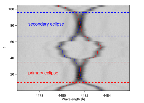
Figure 2.— Spectroscopic observations of CV Vel. Grayscale depiction of the spectra obtained outside eclipses and during both eclipses. The observations are sorted by orbital phase. The horizontal dashed lines indicate the begin and end of the primary (red) and secondary (blue) eclipses. The dark bands represent absorption lines; the darkest band is the Mg ii line. One can also see the weaker AI iii and S ii lines, at shorter and longer wavelengths, respectively. The small vertical blue and red lines indicate the calculated wavelength position of the central Mg ii line, as expected from orbital motion. The lines overlap at times of eclipses. The discontinuities arise because of uneven coverage in orbital phase.

3. Analysis

To measure the sky-projected obliquities, we take advantage of the Rossiter-McLaughlin (RM) effect, which occurs during eclipses. Below we describe our general approach to analyzing the RM effect. Section 3.1 describes some factors specific to the case of CV Vel. Section 3.2 presents the results.

Model

Our approach is similar to that described in Papers I–IV, where it is described in more detail. The projected obliquity of stellar rotation axes can be derived from the deformations of stellar absorption lines during eclipses, when parts of the rotating photospheres are blocked from view, as the exact shape of the deformations depend on the geometry of the eclipse.

We simulate spectra containing light from two stars. The simulated spectra are then compared to the observed spectra, and the model parameters are adjusted to provide the best fit. Our model includes the orbital motion of both stars, and the broadening of the absorption lines due to rotation, turbulent velocities, and the point-spread function of the spectrograph (PSF). For observations made during eclipses, the code only integrates the light from the exposed portions of the stellar disks. The resulting master absorption line (which we will call the “kernel”) is then convolved with a line list which we obtain from the Vienna Atomic Line Database (VALD; Kupka et al., 1999). The lines are shifted in wavelength space according to their orbital radial velocity, and weighed by the relative light contribution from the respective stars. The model is specified by a number of parameters.

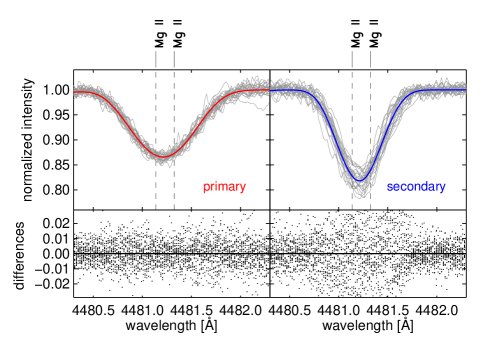
Figure 3.— Absorption lines of CV Vel in 2001/2002. Left.—The lines of the primary, in the region spanning the Mg ii line. The best-fitting model for the secondary lines has been subtracted. Thin gray lines show all the out-of-eclipse observations. The red line shows our model for the primary lines. The lower panel shows the difference between individual observations and the mean line. Right.—The lines of the secondary, after subtracting the model of the primary lines. The blue line shows our model for the secondary. The pulsations of the secondary cause a larger scatter in the residuals. These spectra were obtained in December 2001 and January 2002 with the CORALIE spectrograph by Yakut et al. (2007). Note that (Yakut et al., 2007) mislabeled the primary as the secondary, and vice versa; here we have labeled the spectra correctly. See also (Yakut et al., 2014).

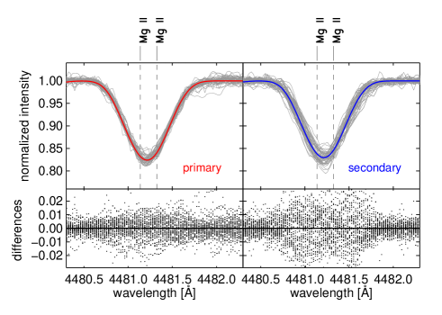
Figure 4.— Absorption lines of CV Vel in 2009/2010. Same as Fig. 3 but for our FEROS and CORALIE spectra obtained outside of eclipses. Comparison to Fig. 3 reveals that the primary absorption lines became significantly narrower between 2001/2002 and 2009/2010.

Model parameters

The orbit is specified by the eccentricity ($e$), argument of periastron ($\omega$), inclination ($i_{o}$), period ($P$), and RV semi-amplitudes of the primary and secondary stars ($K_{\rm p}$ and $K_{\rm s}$). The position of the stars on their orbits, and therefore the times of eclipses, are defined by a particular epoch of primary mid-eclipse ($T_{\rm min,I}$). In addition, additive velocity offsets ($\gamma_{\rm i}$) are needed.

To calculate the duration of eclipses and the loss of light, we need to specify the fractional radius ($r\equiv R/a$, where $a$ is the orbital semimajor axis) and quadratic limb darkening parameters ($u_{1}$ and $u_{2}$) for each star, as well as the light ratio between the two stars ($L_{\rm s}/L_{\rm p}$) at the wavelength of interest.

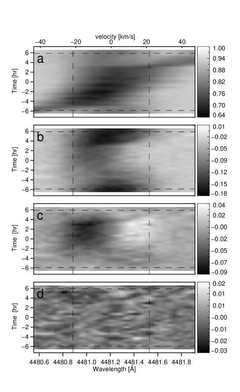
Figure 5.— Observations of CV Vel during primary eclipse. (a) Grayscale depiction of the time dependence of the Mg ii lines of both stars, obtained throughout primary eclipses. The spectra have been shifted into the rest frame of the primary. Horizontal dashed lines mark the approximate boundaries of the primary lines, and vertical dashed lines mark the start and end of the eclipse. (b) After subtracting the secondary lines, based on the best-fitting model (See also Figure 7). (c) After further subtracting a model of the primary lines which does not account for the RM effect, but only the light loss during eclipse. This exposes the deformations due to the RM effect. Darkness indicates a deeper absorption line, lightness indicates a shallower depth than expected in the zero-RM transit model. Throughout most of the primary eclipse, the blueshifted side of the absorption line is deeper, indicating that the companion is almost exclusively eclipsing the receding half of the primary star. From this we can conclude that the primary rotation axis and the orbital axis are misaligned. (d) After subtracting a model including the RM effect.

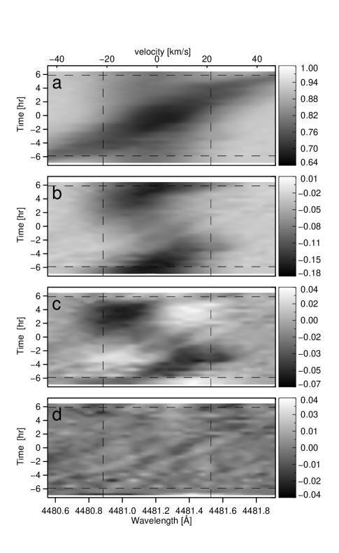
Figure 6.— Observations of CV Vel during secondary eclipse. Similar to Figure 5, but for spectra obtained during secondary eclipses. In contrast to the deformations observed during primary eclipse, here the RM effect is antisymmetric in time and covers the full $v\sin i_{\star}$ range, indicating alignment between the rotational and orbital axes on the sky.

The kernel depends on various broadening mechanisms. Assuming uniform rotation, the rotational broadening is specified by $v\sin i_{\star}$. Turbulent velocities of the stellar surfaces are described with the micro-macro turbulence model of Gray (2005). For this model two parameters are required: the Gaussian width of the macroturbulence ($\zeta_{\rm i}$); and the microturbulence parameter, which is degenerate with the width of the spectrograph PSF. We specify the sky-projected spin-orbit angles ($\beta_{\rm p}$ and $\beta_{\rm s}$) using the coordinate system (and sign convention) of Hosokawa (1953).

Normalization

To take into account the uncertainties due to imperfect continuum normalization, we add 2 free parameters for each spectrum, to model any residual slope of the continuum as a linear function of wavelength. The parameters of the linear function are optimized (in a separate minimization) every time a set of global parameters are evaluated. This process is similar to the “Hyperplane Least Squares” method that was described by Bakos et al. (2010) and used in the context of eclipses in double star systems by Albrecht et al. (2013).

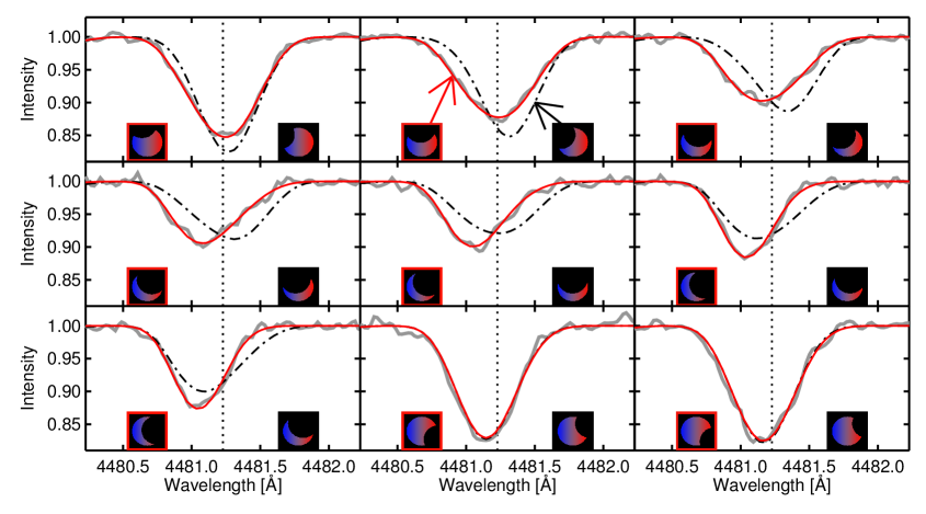
Figure 7.— Absorption lines of CV Vel during primary eclipse. Each panel shows the Mg ii line of the primary star for a particular eclipse phase. The solid gray lines indicate the obtained spectra after subtraction of the best fitting model for the secondary and shifting the system in the restframe of the primary. The central wavelength of the Mg ii line is indicated by the dashed line at $4481.228$ Å. These nine panels show a subset of the observation presented in Figure 5 and are presented in a way equivalent to panel (b). We also show our best fitting primary model as red solid line and as black dash-dotted line a model assuming co-aligned stellar and orbital axes, representing the data poorly. Each panel has two insets depicting the projected rotational velocity of the uncovered surface of the primary star, with blue and red indicating approaching and receding velocities, respectively. The left insets show the model with the misaligned stellar axis, and the right insets show the same for the co-aligned model.

Parameter estimation

To obtain parameter uncertainties we used a Markov Chain Monte Carlo (MCMC) code. Our stepping parameters were as listed above, except that instead of $i_{o}$ we stepped in $\cos i_{o}$, and for the eccentricity parameters we stepped in $\sqrt{e}\cos\omega$ and $\sqrt{e}\sin\omega$. The chains consisted of $0.5$ million calculations of $\chi^{2}$. The results reported below are the median values of the posterior distribution, and the uncertainty intervals are the values which exclude $15.85$ % of the values at each extreme of the posterior and encompass $68.3$ % of the posterior probability.

3.1. Implementation of the model for CV Vel

For CV Vel we focused on the Mg ii line at $4481$ Å, as this line is relatively deep and broadened mainly by stellar rotation. The projected stellar rotation speeds of both stars are small (Table 2). This means that the Mg ii line is well separated from the pressure-broadened He i line at $4471$ Å, simplifying our analysis compared to Papers II–IV. In addition to the Mg ii line, an Al iii doublet and a S ii line are present in our spectral window from $4476$ Å to $4486$ Å. Thus we include these lines in our model. Figure 2 shows a grayscale representation of all our observations in this wavelength range.

Yakut et al. (2007) reported that the two members of the CV Vel system belong to the class of slowly pulsating B stars (Waelkens, 1991). Using CORALIE spectra from December 2001 and January 2002, they observed pulsations in both stars, with the pulsation amplitude for the primary being larger than for the secondary (see their Figure 5c). We reanalyzed their spectra and found that they had mislabeled the primary as the secondary, and vice versa. It is the secondary star which showed the larger pulsations in their CORALIE spectra. In addition, the values of $v\sin i_{\star}$ quoted by Yakut et al. (2007) were assigned to the wrong stars (Yakut et al., 2014). In fact, their measurement of $v\sin i_{\star}=31\pm 2$ km s^-1 belongs to the primary, and their measurement of $v\sin i_{\star}=19\pm 1$ km s^-1 belongs to the secondary. See Figure 3. Our observations took place about a decade later. We also observed large pulsations in the spectra of the secondary star (Figure 4). Here we describe how we dealt with the pulsations while determining the projected obliquIties.

The pulsation period is a few days. The out-of-eclipse observations spanned many months, averaging over many pulsation periods. Thus the pulsations likely introduce additional scatter into the derived orbital parameters, but probably do not introduce large systematic biases in the results. The situation is different for observations taken during eclipses. Over the relatively short timespan of an eclipse, the spectral-line deformation due to pulsation is nearly static or changes coherently, and can introduce biases in the parameters which are extracted from eclipse data. This is true not only for the parameters of the pulsating star, but also for the parameters of the companion star, since the light from both stars is modeled simultaneously. Given the S/N of our spectra, the pulsations of the primary star are too small to be a concern, but the pulsations of the secondary need to be taken into account.

The effects of pulsations are most noticeable in the first two moments of the absorption lines: shifts in the wavelength, and changes in line width. We therefore decided to allow the first two moments of the secondary lines to vary freely for each observation obtained during a primary or secondary eclipse. Each time a trial model is compared to the data the position and width of the lines are adjusted. This scheme is similar to the scheme for the normalization, but now focusing on the lines of the secondary measured during eclipses. The average shift in velocity is about $2$ km s^-1 and never larger than $3$ km s^-1. The changes in width are always smaller then 2%.

Table 2Results for the CV Vel system.

Parameter	This work		Literature values
Orbital parameters
Time of primary minimum, Tmin,I (BJD$-$2 400 000)	42048.66944$\pm$	0.00006	42048.66947$\pm$	0.000141a
Period, $P$ (days)	6.8894976$\pm$	0.00000008	6.889494$\pm$	0.0000081
Cosine of orbital inclination, $\cos i_{o}$	0.0060$\pm$	0.0003
Orbital inclination, $i_{o}$ (deg)	86.54$\pm$	0.02	86.59$\pm$	0.051
Velocity semi-amplitude primary, $K_{\rm p}$ (km s-1)	126.69$\pm$	0.035(stat)$\pm$0.1(sys)	127.0$\pm$	0.22
Velocity semi-amplitude secondary, $K_{\rm s}$ (km s-1)	129.15$\pm$	0.035(stat)$\pm$0.1(sys)	129.1$\pm$	0.22
Velocity offset, $\gamma_{p}$ (km s-1)	24.4$\pm$0.1 23.2$\pm$0.2b		23.9$\pm$	0.33
Velocity offset, $\gamma_{s}$ (km s-1)	24.6$\pm$0.1 23.3$\pm$0.2b		24.3$\pm$	0.43
Orbital semi-major axis, $a$ ($R_{\odot}$)	34.9$\pm$	0.02	34.90$\pm$	0.152
Stellar parameters
Light ratio at 4480 Å, $L_{\rm s}/L_{\rm p}$	0.954$\pm$	0.003	0.90$\pm$	0.021
Fractional radius of primary, $r_{\rm p}$	0.1158$\pm$	0.0002c	0.117$\pm$	0.0011
Fractional radius of secondary, $r_{\rm s}$	0.1139$\pm$	0.0002c	0.113$\pm$	0.0011
$u_{1,\rm i}$+$u_{2,\rm i}$	0.35$\pm$	0.1	(0.341+0.074)$\pm$0.12c
Macroturbulence broadening parameter, $\zeta$ (km s-1)	2.3$\pm$	0.5d
Microturbulence $+$ PSF broadening parameter (km s-1)	8.2$\pm$	0.1d
Projected rotation speed, primary, $v\sin i_{\rm p}$ (km s-1)	21.5$\pm$	0.3$\pm$2	See Table 3
Projected rotation speed, secondary, $v\sin i_{\rm s}$ (km s-1)	21.1$\pm$	0.2$\pm$2	See Table 3
Projected spin-orbit angle, primary, $\beta_{\rm p}$ (∘)	$-52.0$$\pm$	$0.7$$\pm$6
Projected spin-orbit angle, secondary, $\beta_{\rm s}$ (∘)	$3.7$$\pm$	$1.4$$\pm$7
Primary mass, $M_{\rm p}$ ($M_{\odot}$)	6.067$\pm$	0.011d	6.066$\pm$	0.0742
Secondary mass, $M_{\rm s}$ ($M_{\odot}$)	5.952$\pm$	0.011d	5.972$\pm$	0.0702
Primary radius, $R_{\rm p}$ ($R_{\odot}$)	4.08$\pm$	0.03e	4.126$\pm$	0.0242
Secondary radius, $R_{\rm s}$ ($R_{\odot}$)	3.94$\pm$	0.03e	3.908$\pm$	0.0272
Primary $\log g_{\rm p}$ (cgs)	4.000$\pm$	0.008	3.99$\pm$	0.011
Secondary $\log g_{\rm s}$ (cgs)	4.021$\pm$	0.008	4.03$\pm$	0.011
Notes —
a We have placed the HJDUTC value $2442048.66894$ given by Clausen & Gronbech (1977) onto the BJDTDB system.
The two systems differ by $46$ seconds ($0.00053$ days) for this particular epoch.
b The first value was calculated using the VALD line list; the second value was based on the rest frame wavelengths
given by Petrie (1953), provided here for continuity with previous works.
c Value was used as prior.
d See text for a discussion on the uncertainties
e Adopting a solar radius of $6.9566\cdot 10^{8}$ m.
References —
(1) Clausen & Gronbech (1977) (2) Yakut et al. (2007) (3) Andersen (1975)

Along with the spectroscopic data, we fitted the photometric data described in Section 2. Because the eclipses last nearly $12$ hr the data was obtained during different nights and cover large ranges in airmass. We found that, even after performing differential photometry on several comparison stars, the measured flux exhibits significant trends with airmass. Therefore, for each nightly time series, we added two parameters describing a linear function of airmass which were optimized upon each calculation of $\chi^{2}$. As mentioned in Section 2 we also fitted the Strömgren uvby photometry from Clausen & Gronbech (1977).

To constrain the quadratic limb darkening parameters $u_{1,\rm i}$ and $u_{2,\rm i}$ for the relevant bandpasses, we used the ’jktld’ tool to query the predictions of ATLAS atmosphere models (Claret, 2000). We queried the models for the spectroscopic region (around $4500$ Å), the ’Ic’ band, and the Strömgren uvby observations by Clausen & Gronbech (1977). We placed a Gaussian prior on $u_{1}+u_{2}$ with a width of $0.1$ and held the difference $u_{1}-u_{2}$ fixed at the tabulated value. As the two known members of the CV Vel system are of similar spectral type we used the same values for $\zeta$, $u_{1}$, $u_{2}$, and the line strengths for both components.

Similar to the other groups who studied this system, we do not find any sign of an eccentric orbit during our initial trials. We therefore decided to set $e\equiv 0$, in agreement with the results by Clausen & Gronbech (1977), who had gathered the most complete eclipse photometry of the system to date. We found no sign of a systemic drift in $\gamma$ over the three years of observations, and therefore we did not include a linear drift term in our model. However, this does not translate into a stringent constraint on the presence of a potential third body, because most of our observations took place in 2010/2011. As described above, we used the line list from VALD in our model. To derive results which can be compared with earlier works, we also ran our model using the rest wavelengths given by Petrie (1953). For the obliquity work we prefer the VALD line list, as it allows us to treat the Mg ii as doublet, which is important because of the relatively slow rotation in CV Vel (Figure 4). Table 2 presents the $\gamma$ values from both runs.

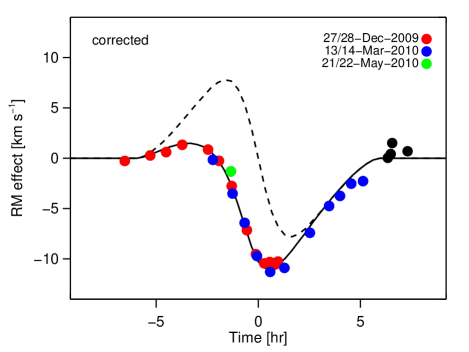
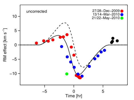
Figure 8.— Anomalous RVs during primary eclipses of CV Vel. Left.—Apparent RV of the primary, after subtraction of the best-fitting orbital model. The solid line is the best-fitting model for the RM effect. The dashed line indicates the expected signal for a well-aligned system. Right.—Same, but neglecting any correction for pulsations of the secondary.

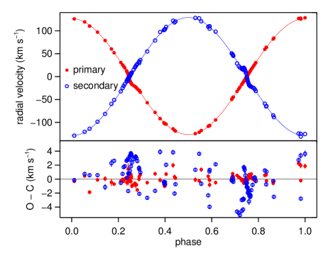
Figure 9.— Orbit of CV Vel Top.—Apparent RVs for the primary and secondary stars in the CV Vel system. This plot is similar to Figure 8 but now for all RVs taken 2009-2013. These RVs are shown for illustrative purposes only and are not used in the analysis of the system. Bottom.— RVs minus best fitting model from the fit to the line shapes. The secondary star exhibits, due to its larger pulsations (Figure 4), a larger RV scatter than the primary star.

3.2. Results

The results for the model parameters are given in Table 2. Figure 5 shows a grayscale representation of the primary spectra in the vicinity of the Mg ii line during the eclipse. Figures 6 shows the same for the spectra obtained during secondary eclipses. Figure 7 presents a subset of primary eclipse observations in a more traditional way.

Concerning the orbital parameters, we find results that are consistent with earlier works. The uncertainties in the fractional stellar radii are small, with significant leverage coming from the spectroscopic eclipse data. Since we have not fully explored how the pulsations in the absorption lines influence our results for the scaled radii, for the purpose of calculating absolute radii we have taken the conservative approach of using the previously determined fractional radii, which have larger uncertainties from (Clausen & Gronbech, 1977, $r_{p}=0.117\pm 0.001$ and $r_{p}=0.113\pm 0.001$). We have not tested how the exact timing of the observations in combination with the pulsations might influence the results for the velocity semi-amplitudes and suggest that $0.1$ km s^-1 is a more realistic uncertainty interval for $K_{\rm i}$ then the statistical uncertainty of $0.035$ km s^-1. We use the enlarged uncertainties in calculating the absolute dimensions of the system. The results for the macroturbulent width $\zeta$ and the microturbulent/PSF width are strongly correlated. The inferred breakdown between these types of broadening depends on our choice of limb darkening parameters. At this point we can only say that any additional broadening beyond rotation is about $8-9$ km s^-1.

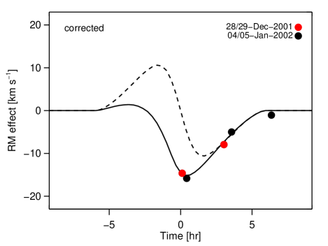
Figure 10.— Anomalous RVs during primary eclipses 2001/2002 in the CV Vel system. Same as Figure 8, but for the data from 2001/2002 obtained by Yakut et al. (2007). Note the larger scale of the $y$-axis compared to the two panels in Figure 8. This is because the $v\sin i_{\star}$ of the primary was higher during 2001/2002.

Projected obliquities and projected rotation speeds

We find that the sky projection of the primary rotation axis is misaligned against the orbital angular momentum, with $\beta_{\rm p}=-52.0\pm 0.7^{\circ}$. The projection of the secondary axis appears to be aligned ($\beta_{\rm s}=3.7\pm 1.4^{\circ}$).

Our method of correcting for pulsations of the secondary turned out to be important, but even with no such corrections the result of a misaligned primary is robust. This is illustrated in Figure 8, which shows the anomalous RVs during primary eclipse. To create this figure we subtracted our best-fitting model of the secondary spectrum from each of the observed spectra. We then measured the RV of the primary star at each epoch, by fitting a Gaussian function to the Mg ii line. We then isolated the RM effect by subtracting the orbital RV, taken from the best-fitting orbital model. The right panel in Figure 8 shows the results for the case when no correction was made for pulsations. There is evidently scatter between the results from different nights, but the predominance of the blueshift throughout the transit implies a misaligned system (a formal fit gives $\beta_{\rm p}=-37^{\circ}$ and $\beta_{\rm s}=-1^{\circ}$). The left panel shows the results for the case in which we have corrected for the time variations in the first two moments of the secondary lines. The scatter is much reduced and the fit to the geometric model is much improved.

Figure 9 shows for completeness all RVs obtained. As mentioned above the RVs out of eclipse have not been corrected for the influence of pulsations. None of the RVs are used in the analysis they are shown here for comparison only.

We further repeated our analysis on two additional lines, the Si iii line at $4552.6$ Å and the He I line at $6678$ Å. For Si iii we obtain $\beta_{\rm p}=-58^{\circ}$ and $\beta_{\rm s}=-4^{\circ}$, and for He I we measure $\beta_{\rm p}=-52^{\circ}$ and $\beta_{\rm s}=-1^{\circ}$. The Si iii line is weaker than the Mg ii line and the He I is pressure broadened, which make the analysis more complex (Albrecht et al., 2011). We therefore prefer the result from the Mg ii line. However we judge that the total spread in the results $6^{\circ}$ and $7^{\circ}$ are probably closer to the true uncertainty in the projected obliquities, than our formal errors. This is because our formal uncertainty intervals rely on measurements taken during 3 and 4 nights, for the primary and secondary, respectively. For a better uncertainty estimation measurements obtained during more different nights, or a more carefully handling of the pulsations, would be needed.

Table 3Projected rotation speed measurements in the in CV Vel system.

Year	$1973$		$2001-2002$		$2009-2010$
Ref.	Andersen (1975)		Yakut et al. (2007)		This work
$v\sin i_{\rm p}$ (km s-1)	28$\pm$	3	29.5$\pm$	$2^{\rm a}$	21.5$\pm$	2
$v\sin i_{\rm s}$ (km s-1)	28$\pm$	3	19.0$\pm$	$2^{\rm a}$	21.1$\pm$	2
Notes —
aBased on our own analysis of the Yakut et al. (2007) spectra.

For the projected rotation speeds we find $v\sin i_{\rm p}=21.5\pm 0.3$ km s^-1 and $v\sin i_{\rm s}=21.1\pm 0.2$ km s^-1. Making the same measurement in the Si iii lines one would obtain $v\sin i_{\rm p}=20.6$ km s^-1 and $v\sin i_{\rm s}=20.0$ km s^-1. For similar reasons as mentioned above for the projected obliquity we suspect that also the formal uncertainties for $v\sin i_{\star}$ are underestimated. In what follows we assume that an uncertainty of $2$ km s^-1 is appropriate.

Yakut et al. (2007) obtained $4$ of their $30$ observations during primary eclipses. We performed a similar analysis of their spectra, in the same manner as our own data. For the projected obliquity of the primary star in 2001/2002 we obtained $\beta_{\rm p\,2002}=-55\pm 3^{\circ}$. As this result rests mainly on two observations, obtained nearly at the same eclipse phase (Figure 10), we judge that the true uncertainty is much larger, probably about $15^{\circ}$. For the projected rotation speeds we obtained $v\sin i_{\rm p\,2002}=29.5\pm 2$ km s^-1 and $v\sin i_{\rm s\,2002}=19.0\pm 2$ km s^-1, adopting a conservative uncertainty interval as we did for our spectra.

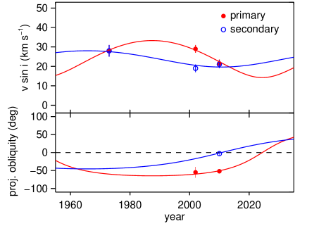
Figure 11.— Precession of the stellar rotation axes in the CV Vel system. The upper panel shows the measured $v\sin i_{\star}$ values of the primary (red solid symbol) and secondary (blue open symbol) stars. The lines indicate the time evolution in our best-fitting model. The lower panel shows the measurements of $\beta$ and the predictions of our model.

4. Rotation and Obliquity

4.1. Precession of the Rotation Axes

Our results for $v\sin i_{\star}$ differ from the values found by Andersen (1975) and from the values found by Yakut et al. (2007) (see Table 3). Evidently the projected rotation rates are changing on a timescale of decades. We are only aware of a few cases in which such changes have been definitively observed, one being the DI Her system (Reisenberger & Guinan, 1989; Albrecht et al., 2009; Philippov & Rafikov, 2013).

Yakut et al. (2007) used the CORALIE spectrograph on the $1.2$ m Swiss telescope for their observations. To exclude any systematic effects due to the choice of instrument—as unlikely as it might seem—we also collected a number of spectra with the CORALIE spectrograph, as described in Section 2, which confirmed the time variation of the $v\sin i_{\star}$ of the primary. The line width of the secondary appears to have changed between the observations conducted by Andersen (1975) and Yakut et al. (2007).

Assuming that $v$ remained constant over the interval of observations ($\sim 30$ yr), we interpret these results as variations in $\sin i_{\star}$ for both stars. This allows us to learn about the precession rates of the stellar rotation axes around the total angular momentum vector of the system. Employing the formulas from Reisenberger & Guinan (1989) we can use the $v\sin i_{\star}$ values from Table 3 together with our measurements of the projected obliquity to obtain values for the stellar obliquities ($\psi$) and rotation velocities of the two stars.

For this purpose, in addition to the system parameters of CV Vel which are presented in Table 3, we need values for the apsidal motion constant ($k_{2}$) and the radius of gyration ($\theta$) of each star. These we obtain from the tables presented by Claret (2004). We use the model with a mass of $6.3$ M_⊙, close to the mass of the stars in the CV Vel system, and estimate the uncertainty by considering the age interval from $30-50$ Myr. The age of CV Vel is estimated to be $40$ Myr (Yakut et al., 2007). The results for both stars are $k_{2}=0.005\pm 0.002$ and $\theta=0.044\pm 0.012$.

Using these values we carried out a Monte Carlo experiment, in which we draw system parameters by taking the best-fitting values and adding random Gaussian perturbations with a standard deviation equal to the 1$\sigma$ uncertainty. For each draw, we minimize a $\chi^{2}$ function by adjusting $\psi$ and $v$ for each star, as well as the particular times when the spin and orbital axes are aligned on the sky. Furthermore we allow the $k_{2}$ and $\theta$ values to vary with a penalty function given by the prior information mentioned above. The resulting parameters are presented in Table 4. In Figure 11 we show the data for $v\sin i_{\star}$ and $\beta$, as well as our model for their time evolution. We obtain $\psi_{\rm p}=67\pm 4^{\circ}$ and $\psi_{\rm s}=46\pm 9^{\circ}$ for the obliquities, and $v_{\rm p}=35\pm 5$ km s^-1 and $v_{\rm s}=28\pm 4$ km s^-1 for the rotation speeds.

The formal uncertainties for $\psi$ and $v$ should be taken with a grain of salt. We did not observe even half a precession period, which makes an estimation of $\psi$ and $v$ strongly dependent on our assumptions regarding $k_{2}$ and $\theta$. We have only a small number of measurements: $3$ $v\sin i_{\star}$ and one or two $\beta$ measurement per star, amounting to $9$ data points. With these we aim to constrain $6$ parameters: $v$, $\psi$, and a reference time for each star. In this situation we can determine parameter values, but we cannot critically test our underlying assumptions. For the secondary in particular we have only little information to constrain $\psi$ and $v$. The only indication we have for this star that it is not aligned is the change in $v\sin i_{\star}$ between 1973 and 2001/2002. Clearly, future observations would be helpful to confirm the time variations. Measurements of the projected obliquity in only a few years should be able to establish if this star’s axis is indeed misaligned (Figure 11). Finally we obtain somewhat different values for $k_{2}$ and $\theta$ for the two stars, which have similar masses and the same age. This is because for the primary the fast change in $v\sin i_{\star}$ between 2002 and 2010 requires a fast precession timescale.

Table 4Precession of the stellar axes in CV Vel

Parameter	CV Vel
Rotation speed of primary $v_{p}$ (km s-1)	33$\pm$	4
Rotation speed of secondary $v_{S}$ (km s-1)	28$\pm$	4
Obliquity of primary $\psi_{\rm p}$ (∘)	$64$$\pm$	4
Obliquity of secondary $\psi_{\rm s}$ (∘)	$46$$\pm$	9
Year when $\beta_{\rm p}=0^{\circ}$	2023$\pm$	7
Year when $\beta_{\rm s}=0^{\circ}$	2011$\pm$	4
Radius of gyration of primary $\theta_{\rm p}$	0.0363$\pm$	0.0095
Radius of gyration of secondary $\theta_{\rm s}$	0.0451$\pm$	0.0009
Apsidal motion constant of primary $k_{2,{\rm p}}$	0.0063$\pm$	0.0007
Apsidal motion constant of secondary $k_{2,{\rm s}}$	0.0047$\pm$	0.0003
Precession period of primary (yr)	139$\pm$	54⋆
Precession period of secondary (yr)	177$\pm$	22⋆

The last point could reflect a shortcoming of our simple model (some missing physics), an underestimation of the errors in the $v\sin i_{\star}$ measurements or the presence of a third body. Nevertheless the finding of a large projected misalignment for the primary and the changes in $v\sin i_{\star}$ measured for both stars makes it difficult to escape the conclusion that the stars have a large obliquity and precess, even if the precise values are difficult to determine at this point. A more detailed precession model and more data on $\beta$ and $v\sin i_{\star}$, obtained over the next few years, would help in drawing a more complete picture.

We note that in principle, one can also use the effect of gravity darkening on the eclipse profiles to constrain $\psi$, as was done recently by Szabó et al. (2011), Barnes et al. (2011) and Philippov & Rafikov (2013) for the KOI-13 and DI Her systems. However as the rotation speed in CV Vel is a factor few slower then in these two systems this would require very precise photometric data. We also note that small changes in the orbital inclination of CV Vel are expected, as another consequence of precession. This might be detected with precise photometry obtained over many years.

4.2. Time evolution of the spins

With an age of $40$ Myr (Yakut et al., 2007) CV Vel is an order of magnitude older than the even-more misaligned system DI Her ($4.5\pm 2.5$ Myr, $\beta_{p}=72\pm 4^{\circ}$ $\beta_{s}=-84\pm 8^{\circ}$, Albrecht et al. 2009; Claret et al. 2010). In this section we investigate if CV Vel could have evolved from a DI Her-like configuration, through the steady action of tidal dissipation. If so, CV Vel might represent a link between young systems with large misalignment, and older systems where tidal interactions have had enough time to attain the equilibrium condition of a circular orbit with aligned and synchronized spins.

In Paper IV, we found that the EP Cru system (age $57\pm 5$ Myr) could not have evolved out of a DI Her like system, despite the strong similarities of all the system parameters except the stellar obliquity and age. This is because the $v\sin i_{\star}$ values in EP Cru are about $9$ times the expected value for the pseudosynchronized state. Theories of tidal interactions predict that damping of any significant spin-orbit misalignment should occur on a similar same time scale as synchronization of the rotation (Hut, 1981; Eggleton & Kiseleva-Eggleton, 2001). This is because in these tidal models, a single coefficient describes the coupling between tides and rotation. If the stellar rotation frequency is much larger than the synchronized value, then rotation around any axis is damped at about the same rate. Therefore while the rotation speed is reduced, the angle between the overall angular momentum and stellar rotation axis does not change. When the stellar rotation around the axis parallel to the orbital angular momentum approaches the synchronized value, then rotation around this axis becomes weakly coupled to the orbit. Tidal damping of rotation around any other axis will only cease when the rotation around these axes stops, and the stellar spin is aligned with the orbital axis. Therefore, finding a system in an aligned state that is rotating significantly faster than synchronized rotation indicates, according to these tidal theories, that the alignment was primordial. In Paper III, we found that NY Cep is also inconsistent with having evolved from a state with large misalignment.

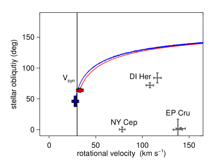
Figure 12.— Tidal evolution of CV Vel. The red and blue crosses mark the derived rotation speeds and obliquities of the primary and secondary. Red and blue lines show the theoretical obliquity evolution of a system like CV Vel. Here we used the currently measured values for CV Vel and evolved the system back in time. The model includes the evolutionary changes in stellar radius with time, and adopts a viscous timescale ($t_{\rm V}$) of 300 000 yr, about 6 000 times larger than what is normally assumed for late type stars. A lower value of $t_{\rm V}$ would lead to an overall faster tidal evolution. It will leave the ratio of the alignment and synchronization timescales unchanged. According to these simulations and measurements it is conceivable that CV Vel had larger (DI Her-like) misalignments when it was younger, and is currently undergoing tidal realignment. The vertical line indicates the synchronized rotation speed ($V_{\rm syn}$) for the current orbital configuration and stellar radii of CV Vel. We also show the measured $v\sin i_{\star}$ and $\beta_{\star}$ for DI Her, NY Cep, and EP Cru, three other systems from the BANANA survey. While the exact value of $V_{\rm syn}$ for these systems differ from the value for CV Vel, all these systems do rotate significantly faster than their synchronized or pseudosynchronized values.

For CV Vel, synchronized rotation would correspond to $v\approx 30$ km s^-1 for both stars. The slow rotation speeds and misaligned axes suggest that we are observing this system in a state in which tides are currently aligning the axes. To illustrate we use the TOPPLE tidal-evolution code (Eggleton & Kiseleva-Eggleton, 2001) with the parameters from Table 2 and Table 4 and evolve the system backwards in time. The results are shown in Figure 12. It appears as if the current rotational state of the two stars is consistent with an evolution out of a higher-obliquity state. We reiterate, though, that the rotation speed and obliquity of the lower mass star are rather uncertain. The results of the tidal evolution do depend on the exact parameters we use for CV Vel, taken from the confidence intervals of our measurements. Therefore we can not make strong statements about the exact evolution CV Vel has taken. However the qualitative character of the evolution did remain the same in all of our runs.

CV Vel did evolve out of a state with larger obliquities and faster rotation. Under this scenario, we are seeing the system after only about one obliquity-damping timescale, which implies that only a small fraction of an eccentricity damping timescale has elapsed (due to the angular momentum in the orbit being greater than that in the spins).

This appears to be a counterintuitive result as one would expect that whatever creates high obliquities would also create a high eccentricity, which should still be present, according to our simple simulation. Scenarios involving a third body, may account for the misaligned spins despite tidal damping of the eccentricity. For example Eggleton & Kiseleva-Eggleton (2001) showed that in the triple system SS Lac, with inner and outer orbits non-parallel, the spin orientations of the two inner components could vary on a timescale of just several hundred years.

As long as the inner and outer orbits remain non-coplanar, the inner orbit will precess around the total angular momentum. The orbital precession timescale will most likely be not the same as the precession timescale of the two stars. Therefore the angle between the stellar spins and the orbital plane of the inner orbit can remain large even after many obliquity damping timescales. The system would settle into a Cassini state, with the oblique spins precessing at the same rate as the inner orbit. A pseudo-synchronous spin rate would settle in for the oblique yet circular orbits (e.g. Levrard et al., 2007; Fabrycky et al., 2007). Of course such a scenario remains speculative as long as no third body is searched for and detected.

The state of the obliquities suggests that DI Her and CV Vel have a history which is qualitatively different from the history of NY Cep, and EP Cru. The two later systems had good alignment throughout their main sequence lifetime, while DI Her and CV Vel did at some point acquire a larger misalignment.

5. Summary

We have analyzed spectra and photometry of the CV Vel system, obtained during primary and secondary eclipses as well as outside of eclipses. Taking advantage of the Rossiter-McLaughlin effect, we find that the rotation axis of the primary star is tilted by $-52\pm 6^{\circ}$ against the orbital angular momentum, as seen on the sky. The sky projections of the secondary rotation axis and the orbital axis are well aligned ($3\pm 7^{\circ}$). Furthermore we find that the projected rotation speeds ($v\sin i_{\star}$) of both stars are changing on a timescale of decades. We interpret these changes as a sign of precession of the stellar rotation axes around the total angular momentum of the system. Using the $v\sin i_{\star}$ measurements (ours and literature measurements dating $30$ years back) in combination with our projected obliquity measurements, we calculate the rotation speed ($v$) as well as the true obliquity ($\psi$) of both stars. We find obliquities of $\psi_{\rm p}=64\pm 4^{\circ}$ and $\psi_{\rm s}=46\pm 9^{\circ}$ and rotation speeds of $v_{\rm p}=33\pm 4$ km s^-1 and $v_{\rm s}=28\pm 4$ km s^-1 for the two stars. While the results for the primary star are relatively solid, the results for the secondary star rely on changes in the measured line width only, and need to be confirmed with future spectroscopic observations.

Our results for the stellar rotation in CV Vel are consistent with long-term tidal evolution from a state in which the stars had higher rotation speeds as well as higher obliquities, similar to what we found in the younger binary system DI Her. In this sense it seems plausible that DI Her and CV Vel are two points on an evolutionary sequence from misaligned to aligned systems. Given the simplest tidal theories, the other systems in our sample (NY Cep, and EP Cru) could not have realigned via tides. So far it is not clear what causes the difference between these two groups. Given recent findings that close binaries are often accompanied by a third body, it is tempting to hypothesize that the influence of a third body is the key factor that is associated with a large misalignment. No third body has yet been detected in either the CV Vel nor DI Her systems, nor have these systems been thoroughly searched. Such a search should be a priority for future work.

References

- Albrecht et al. (2009) Albrecht, S., Reffert, S., Snellen, I. A. G., & Winn, J. N. 2009, Nature, 461, 373
- Albrecht et al. (2007) Albrecht, S., Reffert, S., Snellen, I., Quirrenbach, A., & Mitchell, D. S. 2007, A&A, 474, 565
- Albrecht et al. (2013) Albrecht, S., Setiawan, J., Torres, G., Fabrycky, D. C., & Winn, J. N. 2013, ApJ, 767, 32
- Albrecht et al. (2011) Albrecht, S., Winn, J. N., Carter, J. A., Snellen, I. A. G., & de Mooij, E. J. W. 2011, ApJ, 726, 68
- Andersen (1975) Andersen, J. 1975, A&A, 44, 355
- Bakos et al. (2010) Bakos, G. Á., Torres, G., Pál, A., et al. 2010, ApJ, 710, 1724
- Barnes et al. (2011) Barnes, J. W., Linscott, E., & Shporer, A. 2011, ApJS, 197, 10
- Claret (2000) Claret, A. 2000, A&A, 363, 1081
- Claret (2004) —. 2004, A&A, 424, 919
- Claret et al. (2010) Claret, A., Torres, G., & Wolf, M. 2010, A&A, 515, A4
- Clausen & Gronbech (1977) Clausen, J. V., & Gronbech, B. 1977, A&A, 58, 131
- De Cat & Aerts (2002) De Cat, P., & Aerts, C. 2002, A&A, 393, 965
- Eggleton & Kiseleva-Eggleton (2001) Eggleton, P. P., & Kiseleva-Eggleton, L. 2001, ApJ, 562, 1012
- Fabrycky et al. (2007) Fabrycky, D. C., Johnson, E. T., & Goodman, J. 2007, ApJ, 665, 754
- Fabrycky & Tremaine (2007) Fabrycky, D., & Tremaine, S. 2007, ApJ, 669, 1298
- Feast (1954) Feast, M. W. 1954, MNRAS, 114, 246
- Gaposchkin (1955) Gaposchkin, S. 1955, MNRAS, 115, 391
- Gillon et al. (2011) Gillon, M., Jehin, E., Magain, P., et al. 2011, in European Physical Journal Web of Conferences, Vol. 11, European Physical Journal Web of Conferences, 6002
- Gray (2005) Gray, D. F. 2005, The Observation and Analysis of Stellar Photospheres, 3rd Ed. (ISBN 0521851866, Cambridge University Press)
- Hosokawa (1953) Hosokawa, Y. 1953, PASJ, 5, 88
- Hut (1981) Hut, P. 1981, A&A, 99, 126
- Kaufer et al. (1999) Kaufer, A., Stahl, O., Tubbesing, S., et al. 1999, The Messenger, 95, 8
- Kozyreva & Bagaev (2009) Kozyreva, V. S., & Bagaev, L. A. 2009, Astronomy Letters, 35, 483
- Kupka et al. (1999) Kupka, F., Piskunov, N., Ryabchikova, T. A., Stempels, H. C., & Weiss, W. W. 1999, A&AS, 138, 119
- Lai (2012) Lai, D. 2012, MNRAS, 423, 486
- Lehmann et al. (2013) Lehmann, H., Southworth, J., Tkachenko, A., & Pavlovski, K. 2013, A&A, 557, A79
- Levrard et al. (2007) Levrard, B., Correia, A. C. M., Chabrier, G., et al. 2007, A&A, 462, L5
- Mazeh & Shaham (1979) Mazeh, T., & Shaham, J. 1979, A&A, 77, 145
- Naoz et al. (2013) Naoz, S., Farr, W. M., Lithwick, Y., Rasio, F. A., & Teyssandier, J. 2013, MNRAS, 431, 2155
- Pavlovski et al. (2011) Pavlovski, K., Southworth, J., & Kolbas, V. 2011, ApJ, 734, L29
- Petrie (1953) Petrie, R. M. 1953, Publications of the Dominion Astrophysical Observatory Victoria, 9, 297
- Philippov & Rafikov (2013) Philippov, A. A., & Rafikov, R. R. 2013, ApJ, 768, 112
- Reisenberger & Guinan (1989) Reisenberger, M. P., & Guinan, E. F. 1989, AJ, 97, 216
- Rogers et al. (2012) Rogers, T. M., Lin, D. N. C., & Lau, H. H. B. 2012, ArXiv, arXiv:1209.2435 [astro-ph.SR]
- Rogers et al. (2013) Rogers, T. M., Lin, D. N. C., McElwaine, J. N., & Lau, H. H. B. 2013, ApJ, 772, 21
- Shakura (1985) Shakura, N. I. 1985, Soviet Astronomy Letters, 11, 224
- Szabó et al. (2011) Szabó, G. M., Szabó, R., Benkő, J. M., et al. 2011, ApJ, 736, L4
- Torres et al. (2010) Torres, G., Andersen, J., & Giménez, A. 2010, A&A Rev., 18, 67
- Triaud et al. (2013) Triaud, A. H. M. J., Hebb, L., Anderson, D. R., et al. 2013, A&A, 549, A18
- van Houten (1950) van Houten, C. J. 1950, Annalen van de Sterrewacht te Leiden, 20, 223
- van Leeuwen (2007) van Leeuwen, F. 2007, A&A, 474, 653
- Waelkens (1991) Waelkens, C. 1991, A&A, 246, 453
- Yakut et al. (2007) Yakut, K., Aerts, C., & Morel, T. 2007, A&A, 467, 647
- Yakut et al. (2014) —. 2014, A&A, 562, C2
- Zhou & Huang (2013) Zhou, G., & Huang, C. X. 2013, ApJ, 776, L35