The Stagger-grid: A grid of 3D stellar atmosphere models

Abstract

Aims. We investigate the relation between 1D atmosphere models that rely on the mixing-length theory and models based on full 3D radiative hydrodynamic (RHD) calculations to describe convection in the envelopes of late-type stars.

Methods. The adiabatic entropy value of the deep convection zone, $s_{\mathrm{bot}}$, and the entropy jump, $\Delta s$, determined from the 3D RHD models, were matched with the mixing-length parameter, $\alpha_{\mathrm{MLT}},$ from 1D hydrostatic atmosphere models with identical microphysics (opacities and equation-of-state). We also derived the mass mixing-length parameter, $\alpha_{m}$, and the vertical correlation length of the vertical velocity, $C\left[v_{z},v_{z}\right]$, directly from the 3D hydrodynamical simulations of stellar subsurface convection.

Results. The calibrated mixing-length parameter for the Sun is $\alpha_{\mathrm{MLT}}^{\odot}\left(s_{\mathrm{bot}}\right)=1.98$. For different stellar parameters, $\alpha_{\mathrm{MLT}}$ varies systematically in the range of $1.7-2.4$. In particular, $\alpha_{\mathrm{MLT}}$ decreases towards higher effective temperature, lower surface gravity and higher metallicity. We find equivalent results for $\alpha_{\mathrm{MLT}}^{\odot}\left(\Delta s\right)$. In addition, we find a tight correlation between the mixing-length parameter and the inverse entropy jump. We derive an analytical expression from the hydrodynamic mean-field equations that motivates the relation to the mass mixing-length parameter, $\alpha_{m}$, and find that it qualitatively shows a similar variation with stellar parameter (between $1.6$ and $2.4$) with the solar value of $\alpha_{m}^{\odot}=1.83$. The vertical correlation length scaled with the pressure scale height yields $1.71$ for the Sun, but only displays a small systematic variation with stellar parameters, the correlation length slightly increases with $T_{\mathrm{eff}}$.

Conclusions. We derive mixing-length parameters for various stellar parameters that can be used to replace a constant value. Within any convective envelope, $\alpha_{m}$ and related quantities vary strongly. Our results will help to replace a constant $\alpha_{\mathrm{MLT}}$.

1 Introduction

In the past century, insights in various fields of physics led to a substantially more accurate interpretation and understanding of the processes taking place in the interior of celestial bodies. Astronomers can parameterize the conditions on the surface of stars with theoretical stellar atmosphere models, and with the theory of stellar structure and evolution, they are additionally capable to predict the complex development of stars.

The radiated energy of cool stars, originating from the deeper interior because of nuclear burning in the center, is advected to the surface by convective motions in the envelope that are driven by negative buoyancy acceleration. At the thin photospheric transition region the large mean free path of photons allows them to escape into space, and the convective energy flux is abruptly released. To theoretically model this superadiabatic boundary domain of stars is challenging because of the nonlinear and nonlocal nature of turbulent subsurface convection and radiative transfer, and an analytical solution is a long-standing unresolved problem.

To account for the convective energy transport, Böhm-Vitense (1958) formulated the mixing-length theory (MLT), which was initially proposed by Prandtl (1925) in analogy to the concept of the mean free path in the kinetic gas theory. In the framework of MLT, it is assumed that the heat flux is carried by convective elements for a typical distance before they dissolve instantaneously into the background. This distance is the so-called mixing-length, $l$, usually expressed in units of the pressure scale height, $\alpha_{\mathrm{MLT}}=l/H_{P}$. The mixing-length parameter $\alpha_{\mathrm{MLT}}$ is a priori unknown, hence it has to be calibrated, usually by matching the current radius and luminosity of the Sun by a standard solar model with a single depth-independent $\alpha_{\mathrm{MLT}}^{\odot}$. This calibrated value for the Sun is then used for all stellar parameters. We recall that $\alpha_{\mathrm{MLT}}^{\odot}$, in fact, corrects for all other shortcomings of the solar model, deficits in the equation-of-state (EOS), the opacities, or the solar composition. It therefore is no wonder that its numerical value (typically around 1.7 to 1.9; e.g., see Magic et al. 2010) varies with progress in these aspects and from code to code. In addition, MLT is a local and time-independent theory that effectively contains three additional, free parameters, and assumes symmetry in the up- and downflows, hence also in the vertical and horizontal direction. The actual formulation of MLT can also vary slightly (e.g., see Henyey et al. 1965; Mihalas 1970; Ludwig et al. 1999).

Many attempts have been made to improve MLT, a substantial one being the derivation of a nonlocal mixing-length theory (Gough 1977; Unno et al. 1985; Deng et al. 2006; Grossman et al. 1993). The standard MLT is a local theory, meaning that the convective energy flux is derived purely from local thermodynamical properties, ignoring thus any nonlocal properties (e.g., overshooting) of the flow. Nonlocal models are typically derived from the hydrodynamic equations, which are a set of nonlinear moment equations including higher order moments. To solve them, closure approximations are considered (e.g., diffusion approximation, anelatistic approximations, or introducing a diffusion length). Other aspects have also been studied: the asymmetry of the flow by a two-stream MLT model (Nordlund 1976), the anisotropy of the eddies (Canuto 1989), the time-dependence (Xiong et al. 1997), and the depth-dependence of $\alpha_{\mathrm{MLT}}$ (Schlattl et al. 1997). While standard MLT accounts for only a single eddy size (which is $l$), Canuto & Mazzitelli (1991) extended this to a larger spectrum of eddy sizes by including the nonlocal second-order moment (Canuto et al. 1996). The original Canuto-Mazzitelli theory – also known as the full spectrum turbulence model – used the distance to the convective region border as a proxy for the mixing-length; a later version (Canuto & Mazzitelli 1992) re-introduced a free parameter resembling $\alpha_{\mathrm{MLT}}$.

These approaches are often complex, but so far, the standard MLT is still widely in use, and a breakthrough has not been achieved, despite all the attempts for improvements. In 1D atmosphere modeling, the current procedure is to assume a universal value of $1.5$ for the mixing-length parameter $\alpha_{\mathrm{MLT}}$ (Gustafsson et al. 2008; Castelli & Kurucz 2004, see). For full stellar evolution models, the solar “calibration” yields values around $\sim 1.7-1.9$ (Magic et al. 2010, see, e.g. ). Since the value of the mixing-length parameter sets the convective efficiency and therefore changes the superadiabatic structure of stellar models, an accurate knowledge of $\alpha_{\mathrm{MLT}}$ for different stellar parameters would be a first step in improving models in that respect. However, apart from the Sun, other calibrating objects are rare and data are much less accurate (see Sect. 3.7 for an example), such as binary stars with well-determined stellar parameters.

The mixing-length parameter can be deduced from multidimensional radiative hydrodynamic (RHD) simulations, where convection emerges from first principles (e.g., see Ludwig et al. 1999). Over the past decades, the computational power has increased and the steady development of 3D RHD simulations of stellar atmospheres has established their undoubted reliability by manifold successful comparisons with observations (Nordlund 1982; Steffen et al. 1989; Ludwig et al. 1994; Freytag et al. 1996; Stein & Nordlund 1998; Nordlund & Dravins 1990; Nordlund et al. 2009). The 3D RHD models have demonstrated that the basic picture of MLT is incorrect: there are no convective bubbles, but highly asymmetric convective motions. Nonetheless, an equivalent mixing-length parameter has been calibrated by Ludwig et al. (1999) based on 2D hydrodynamic models by matching the resulting adiabats with 1D MLT models (see Freytag et al. 1999, for the metal-poor cases). The authors showed that $\alpha_{\mathrm{MLT}}$ varies significantly with the stellar parameters (from $1.3$ to $1.8$), and also studied the impact of a variable $\alpha_{\mathrm{MLT}}$ on a globular cluster (Freytag & Salaris 1999). In addition, Trampedach (2007) applied a grid of 3D atmosphere models with solar metallicity to calibrate the mixing-length parameter (from 1.6 to 2.0), and the so-called mass mixing-length (Trampedach & Stein 2011).

In the present work we calibrate the mixing-length parameter with a 1D atmosphere code that consistently employs the identical EOS and opacity as used in the 3D RHD simulations (Sect. 2). We present the resulting mixing-length parameter in Sect. 3. We also determine the mass mixing-length – the inverse of the logarithmic derivative of the unidirectional mass flux – in Sect. 4, and the vertical correlation length of the vertical velocity (Sect. 5) directly from the 3D atmosphere models. For the former quantity, we derive a relation from the hydrodynamic mean-field equations that demonstrates the relation to $\alpha_{\mathrm{MLT}}$, which is further substantiated by our numerical results. Finally, we conclude in Sect. 6.

2 Theoretical models

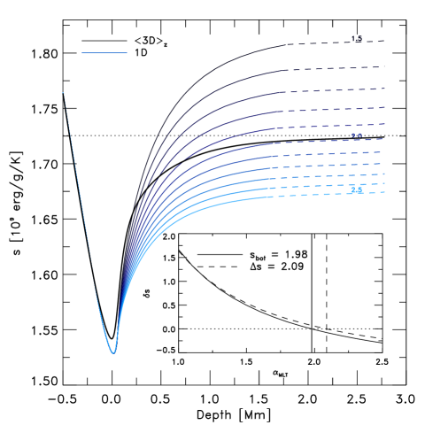
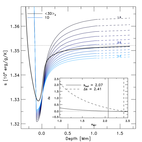
Figure 1: Mean $\left\langle\mathrm{3D}\right\rangle_{z}$ entropy (black solid line) vs. depth, and 1D models for different mixing-length parameters, $\alpha_{\mathrm{MLT}}=1.5-2.5$ (blue lines), for the solar model (left panel) and a metal-poor dwarf with $\left[\mathrm{Fe}/\mathrm{H}\right]-2.0,\,T_{\mathrm{eff}}=4500\,\mathrm{K}$, and $\log g=4.5$ (right panel). We indicate the constant entropy value of the deep adiabatic convection zone, $s_{\mathrm{bot}}$, in both figures by the horizontal dotted line. In the deeper layers, we extended the 1D models (dashed lines) with the aid of the entropy gradient from the $\left\langle\mathrm{3D}\right\rangle$ models. The calibration of the mixing-length parameter $\alpha_{\mathrm{MLT}}$ for the solar model is illustrated by the smaller insets, which depict the relative differences between the 1D and 3D models ($\delta s=s_{1\mathrm{D}}/s_{3\mathrm{D}}-1$) for $s_{\mathrm{bot}}$ (solid) and the entropy jump $\Delta s$ (dashed). For the solar model the two approaches result in $\alpha_{\mathrm{MLT}}=1.98$ and $2.09$.

2.1 3D atmosphere models

We computed the Stagger-grid, a large grid of 3D RHD atmosphere models that covers a wide range in stellar parameter space (see Magic et al. 2013a, hereafter Paper I). The 3D atmosphere models were computed with the Stagger-code, which solves the 3D hydrodynamic equations for conservation of mass, momentum and energy, coupled with a realistic treatment of the radiative transfer. We employed the EOS by Mihalas et al. (1988), and up-to-date continuum and line opacities (Gustafsson et al. 2008). For the solar chemical abundances, we used the values by Asplund et al. (2009, hereafter AGS09). Our simulations are of the so-called box-in-a-star type, that is we compute only a small, statistically representative volume that includes typically ten granules. Our (shallow) simulations only cover a small fraction of the total depth of the convective envelope. Because of the adiabaticity of the gas in the lower parts of the simulation box, the asymptotic entropy value of the convective zone, $s_{\mathrm{ad}}$, is matched by the fixed entropy at the bottom of the simulation domain, $s_{\mathrm{bot}}$, which is one of the simulation parameters. The effective temperature is therefore a result in our 3D simulations, and is actually a temporally averaged quantity. In 1D models $T_{\mathrm{eff}}$ is an actual fixed input value in addition without fluctuations.

We determine the entropy jump, $\Delta s$, as the difference between the entropy minimum and the constant entropy value of the adiabatic convection zone with $\Delta s=s_{\mathrm{min}}-s_{\mathrm{bot}}$. In Magic et al. (2013b, hereafter Paper II), we studied in detail the differences between mean $\left\langle\mathrm{3D}\right\rangle$ models resulting from different reference depth scales. In the present work, we show and discuss only averages on constant geometrical height $\left\langle\mathrm{3D}\right\rangle_{z}$, since these fulfill the hydrodynamic equilibrium and extend over the entire vertical depth of the simulations. The Stagger-grid encompasses $\sim 220$ models ranging in effective temperature, $T_{\mathrm{eff}}$, from $4000$ to $7000\,\mathrm{K}$ in steps of approximately $500\,\mathrm{K}$ (we recall that $T_{\mathrm{eff}}$ is the result of the input quantity $s_{\mathrm{ad}}$, and the intended $T_{\mathrm{eff}}$ grid point values are adjusted within a margin below 100 K). The surface gravity, $\log g$, ranges from $1.5$ to $5.0$ in steps of 0.5 dex, and metallicity, $\left[\mathrm{Fe}/\mathrm{H}\right]$, from $-4.0$ to $+0.5$ in steps of $0.5$ and $1.0\,\mathrm{dex}$. We refer to Paper I for detailed information on the actual methods for computing the grid models, their global properties, and mean stratifications.

2.2 1D atmosphere models

For the Stagger-grid, a 1D MLT atmosphere was developed that uses exactly the same opacities and EOS as the 3D models (Paper I). Therefore, the chemical compositions are identical. The code uses the MLT formulation by Henyey et al. (1965) (see App. C.1 for details), similar to the MARCS code (Gustafsson et al. 2008). Furthermore, for consistency, the 1D models were computed with exactly the same $T_{\mathrm{eff}}$ as the 3D models.

The actual implementation of MLT differs slightly depending on the considered code (e.g., Ludwig et al. 1999). In the standard MLT formulation there are four parameters in total. The mixing-length parameter, $\alpha_{\mathrm{MLT}}=l/H_{p}$, sets the convective efficiency, while $y=3/(4\pi^{2})\simeq 0.076$ is assumed for the temperature distribution, and $\nu=8$ for the turbulent viscosity (see App. C.2 for a discussion). We only considered the mixing-length parameter $\alpha_{\mathrm{MLT}}$ for the calibration, while the additional parameters were kept fixed to their default values, and the turbulent pressure was entirely neglected.

3 mixing-length parameter

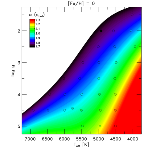
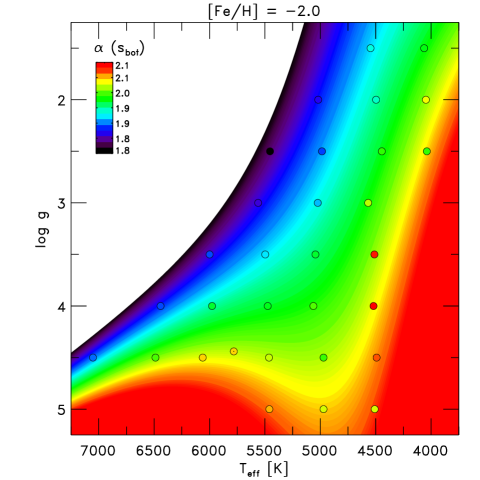
Figure 2: Kiel-diagram ($T_{\mathrm{eff}}-\log g$ diagram) with the mixing-length parameter calibrated with the constant entropy value of the adiabatic convection zone, $\alpha_{\mathrm{MLT}}\left(s_{\mathrm{bot}}\right)$, for solar and subsolar metallicity (left and right panels, respectively). The mixing-length is color-coded as indicated and shown with contours derived from functional fits (see App. B), while the circles represent the Stagger-grid models. Note the difference in the color scales.

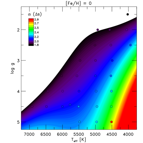
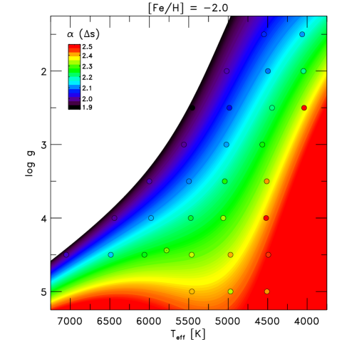
Figure 3: As Fig. 2, but here we show the mixing-length parameter calibrated with the entropy jump $\alpha_{\mathrm{MLT}}\left(\Delta s\right)$.

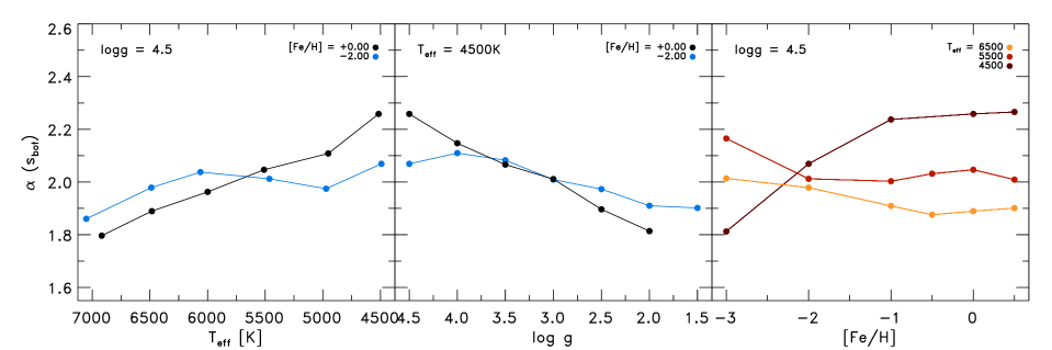
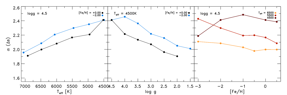
Figure 4: Dependence of the mixing-length parameters on the different stellar parameters ($\alpha_{\mathrm{MLT}}\left(s_{\mathrm{bot}}\right)$ and $\alpha_{\mathrm{MLT}}\left(\Delta s\right)$ in the top and bottom panel, respectively). We varied one stellar parameter at a time, while the other two were kept fixed (left: effective temperature; middle: surface gravity; right: metallicity). The fixed stellar parameters are indicated and color-coded.

3.1 Matching the mixing-length parameter

We calibrated $\alpha_{\mathrm{MLT}}$ by matching either the asymptotic entropy value of the deep convection zone, $s_{\mathrm{bot}}$, or the entropy jump, $\Delta s$, from the 1D and 3D models. We refer to these throughout as $\alpha_{\mathrm{MLT}}\left(s_{\mathrm{bot}}\right)$ and $\alpha_{\mathrm{MLT}}\left(\Delta s\right)$. The value of $s_{\mathrm{bot}}$ is an input parameter in our 3D simulations and represents the adiabatic entropy of the incoming upflows at the bottom of the box that are replenishing the outflows. The horizontally and temporally averaged entropy at the bottom, $\left\langle s\right\rangle_{\mathrm{bot}}$, in contrast, considers both the up- and downflow, and is thus slightly lower than $s_{\mathrm{bot}}$ because of the entropy-deficient downflows. However, in our simulations the deeper layers have almost adiabatic conditions. The contrast of the thermodynamic variables at the bottom is extremely low with $\left\langle X\right\rangle_{\mathrm{bot}}-X_{\mathrm{bot}}\ll 1\,\%$.

For the calibration, we computed 1D models with $\alpha_{\mathrm{MLT}}$ from $1.0$ to $2.5$ in steps of $0.1$ and determined $\alpha_{\mathrm{MLT}}$ by minimizing the difference $\delta s=s_{\mathrm{bot}}^{\mathrm{1D}}-s_{\mathrm{bot}}^{\mathrm{3D}}$ or the difference in the entropy jumps $\delta s=\Delta s^{1\mathrm{D}}-\Delta s^{3\mathrm{D}}$. We remark that some 1D atmosphere models had convergence problems, when they were extended to the same depth as the 3D models. Therefore, we had to calculate slightly shallower 1D models. However, we extended the 1D entropy stratifications with the entropy gradients of the $\left\langle\mathrm{3D}\right\rangle$ model (see Fig. 1). We performed tests by truncating $\left\langle\mathrm{3D}\right\rangle$ models and extending them with our method, which led to the same stratification. Therefore, we assume that the missing depth in the 1D entropy run leads to only minor uncertainties in the resulting $\alpha_{\mathrm{MLT}}$. We fitted the differences, $\delta s$, with a second-order polynom to derive the value of $\alpha_{\mathrm{MLT}}$. We emphasize that the calibration of $\alpha_{\mathrm{MLT}}$ is more meaningful for identical EOS, and the entropy is consistently computed. For the calibration, we neglected the turbulent pressure in the 1D models entirely (i.e., $\beta=0$). Including turbulent pressure would clearly influence the calibration of $\alpha_{\mathrm{MLT}}$, but, to account properly for $p_{\mathrm{turb}}$, one would need to employ an improved description of convection that accounts for nonlocal effects (private communication with D. Gough, and see also Ludwig et al. 2008). Because of the local nature of the standard MLT, the impact of the turbulent pressure is confined to the convective region and the turbulent leviation is rendered poorly. We note that the influence of the turbulent pressure is included in the calibrated $\alpha_{\mathrm{MLT}}$ values.

In Fig. 1, we illustrate the calibration for the solar model and for a cool metal-poor dwarf with the mean entropy, $s$, in the convection zone. For the solar simulation, we determined a mixing-length parameter of $\alpha_{\mathrm{MLT}}=1.98$ and $2.09$ from matching either the adiabatic entropy value (left panel) or the entropy jump (right panel). Note how $s$ converges asymptotically against $s_{\mathrm{bot}}$. Furthermore, it is also evident from Fig. 1 that for a higher $\alpha_{\mathrm{MLT}}$ the adiabat ($s_{\mathrm{bot}}$) of the 1D models is decreasing in the convection zone. The entropy minimum of the $\left\langle\mathrm{3D}\right\rangle_{z}$ on geometrical height is slightly mismatched by the 1D models, which is reflected by slightly different calibrated $\alpha_{\mathrm{MLT}}\left(\Delta s\right)$ values. In the 1D models $s_{\mathrm{min}}$ varies only little for different $\alpha_{\mathrm{MLT}}$, and the differences, $\Delta\alpha_{\mathrm{MLT}}$, are between $\sim 10^{-4}$ and $10^{-3}$ (cf. also the right panel). Since the entropy jumps are in general much larger than the variation of $s_{\mathrm{min}}$, their influence is very weak, and only for very cool metal-poor models with very small entropy jumps, differences in $s_{\mathrm{min}}$ influence the calibration (see right panel in Fig. 1).

We find in general very similar results for $\alpha_{\mathrm{MLT}}$ by employing a 1D envelope code, which solves the stellar structure equations down to the radiative interior by including the same EOS and opacities (Christensen-Dalsgaard 2008). This is in particular true for solar metallicity. The 1D envelope code relies on an assumed $T(\tau)$ relation in the (Eddington gray) atmosphere, which obviously influences the thermal stratification at the outer boundary of the convective envelope. In particular, metal-poor 1D convective interior models with a fixed $T(\tau)$ relation are affected by this, and will return different mixing-length parameters. The 1D atmosphere code works without the need for any $T(\tau)$ relation, since it solves the radiative transfer by itself. We therefore present and discuss only the mixing-length parameters matched by the 1D atmosphere code.

Furthermore, we have performed functional fits for the calibrated mixing-length parameters, that is $\alpha_{\mathrm{MLT}}=f\left(T_{\mathrm{eff}},\log g,\left[\mathrm{Fe}/\mathrm{H}\right]\right)$, with the same functional basis as used by Ludwig et al. (1999). For more details see App. B, and the resulting coefficients are provided in Table 2. In Table 2 we also listed the uncertainties of the fits estimated with the root-mean-square and highest deviation, which are increasing for lower metallicities.

3.2 Calibrations with the adiabatic entropy value

In Fig. 2, we show an overview of the variation of the $\alpha_{\mathrm{MLT}}$ values calibrated with $s_{\mathrm{bot}}$ for different stellar parameters in the Kiel-diagram, in particular, for two illustrating metallicities ($\mathrm{[Fe/H]}=0$ and $-2$). The mixing-length parameter varies rather systematically in the range between $\sim 1.7$ and $\sim 2.3$: $\alpha_{\mathrm{MLT}}$ increases for lower $T_{\mathrm{eff}}$ and $\left[\mathrm{Fe}/\mathrm{H}\right]$ and higher $\log g$ (see also Fig. 4). Towards lower metallicity, models with cooler $T_{\mathrm{eff}}$ deviate from a linear run, which can be attributed to the differences in the outer boundary condition of the 1D models. A larger $\alpha_{\mathrm{MLT}}$ relates to a higher convective efficiency, which implies that a smaller entropy jump is necessary to carry the same convective energy flux. Indeed, we find the entropy jump to increase for higher $T_{\mathrm{eff}}$, lower $\log g$, and higher $\left[\mathrm{Fe}/\mathrm{H}\right]$ (see Paper I); we find that $\alpha_{\mathrm{MLT}}$ varies qualitatively inversely to the entropy jump. The mixing-length parameter is inversely proportional to the variation of the logarithmic values of the entropy jump, the peak in the entropy contrast, and vertical rms-velocity (see Sect. 3.4). This agrees with the fact that both the entropy jump and the mixing-length parameter are related to the convective efficiency (see Sect. 3.4).

3.3 Calibrations with the entropy jump

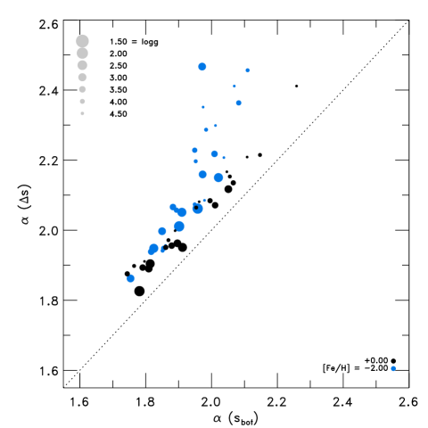
Figure 5: Comparison of the mixing-length parameter calibrated with the entropy jump, $\alpha_{\mathrm{MLT}}\left(\Delta s\right)$, and the constant entropy value of the adiabatic convection zone, $\alpha_{\mathrm{MLT}}\left(s_{\mathrm{bot}}\right)$, for different stellar parameters.

We also calibrated the mixing-length parameter with the 1D MLT atmosphere code by matching the entropy jump $\Delta s$. The resulting values are summarized for two metallicities in Fig. 3, showing a similar behavior as the results of the previous section (see also Fig. 4). We find that the $\alpha_{\mathrm{MLT}}$ values based on $\Delta s$ are systematically higher by $\sim 0.1$ (between $\sim 1.8$ and $\sim 2.4$) than the values based on $s_{\mathrm{bot}}$ (Fig. 5), but the range in $\alpha_{\mathrm{MLT}}\left(\Delta s\right)$ is with $\Delta\alpha_{\mathrm{MLT}}\approx 0.6$ very similar to that for $\alpha_{\mathrm{MLT}}\left(s_{\mathrm{bot}}\right)$. The differences arise from the minimum of the entropy $s_{\mathrm{min}}$ around the optical surface, which is lower for the 1D models than for the $\left\langle\mathrm{3D}\right\rangle$ model (see Fig. 1), and therefore leads to larger mixing-length parameters. The metal-poor simulations deviate more strongly between $\alpha_{\mathrm{MLT}}\left(\Delta s\right)$ and $\alpha_{\mathrm{MLT}}\left(s_{\mathrm{bot}}\right)$, since the boundary effect, induced by the differences in $\Delta s$, increases for lower $\left[\mathrm{Fe}/\mathrm{H}\right]$. We note that the entropy jump is a relative value, and consequently, the matching is less sensitive to outer boundary effects.

3.4 Comparison with global properties

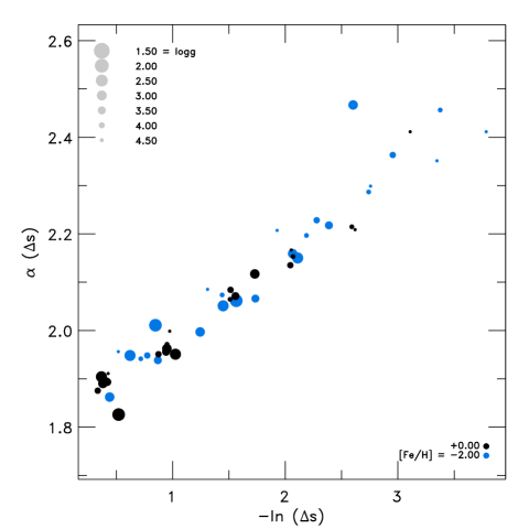
Figure 6: Comparison between the mixing-length parameter calibrated with the entropy jump, $\alpha_{\mathrm{MLT}}\left(\Delta s\right)$, and the logarithm of the inverse of the entropy jump, $-\ln\left(\Delta s\right)$, for different stellar parameters.

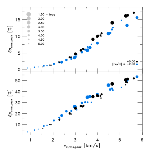
Figure 7: Highest contrast of the entropy and density compared with the highest vertical rms-velocity (top and bottom panel, respectively) for different stellar parameters.

We searched for systematic correlations between the mixing-length parameter and mean thermodynamic properties. The inverse of the entropy jump correlates well with $\alpha_{\mathrm{MLT}}$. In Fig. 6 we demonstrate this by comparing the mixing-length parameter $\alpha_{\mathrm{MLT}}\left(\Delta s\right)$ with the logarithm of the inverse of the entropy jump. Convection is driven by radiative cooling in the surface layers. The entropy jump results from the radiative losses at the optical surface, therefore, the correlation of $\alpha_{\mathrm{MLT}}$ originates in the interplay of the opacity, $\kappa_{\lambda}$, radiative cooling rates, $q_{\mathrm{rad}}$, and vertical velocity, $v_{z,\mathrm{rms}}$. The vertical velocity results from buoyancy forces, $f_{b}=g\Delta\rho$, that act on the overturning, overdense flows at the optical surface. Hence, a larger entropy jump will entail higher contrast in the entropy and density ($\delta s_{\mathrm{rms}}$ and $\delta\rho_{\mathrm{rms}}$), which will induce a stronger downward acceleration. We illustrate this in Fig. 7, where the peak values for $\delta s_{\mathrm{rms}}$ and $\delta\rho_{\mathrm{rms}}$ in the superadiabatic region are plotted against the peak vertical rms-velocity. Evidently, the entropy and density contrast correlate well with the vertical velocity, and this is the underlying reason for the tight (inverse) correlation between mixing-length parameter and entropy jump. In Paper I we have already discussed the correlation of the entropy jump with the peak vertical velocity and the density at the same location, and we deduced the reason for this in the convective energy flux, which essentially contains these quantities.

3.5 Comparison with 2D calibrations

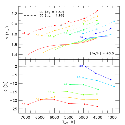
Figure 8: Top panel: calibration of $\alpha_{\mathrm{MLT}}$ with 2D (Ludwig et al. 1999) and 3D simulations in comparison (solid and dashed lines, respectively). The surface gravity is indicated and color-coded. The solar values are indicated. Bottom panel: relative differences ($\delta=2\mathrm{D}/3\mathrm{D}-1$).

We compared the differences between our inferred mixing-length parameters with those of Ludwig et al. (1999) based on similar, but 2D hydrodynamical surface convection simulations. These authors also matched the resulting 2D-based $s_{\mathrm{bot}}$ by varying $\alpha_{\mathrm{MLT}}$ of a 1D envelope code that uses the same EOS and opacity. However, the EOS and opacity are not identical to those used by us, and there are other differences in the models, such as, most importantly, the solar composition. This needs to be kept in mind when interpreting the comparison.

We also remark that Ludwig et al. (1999) derived $T(\tau)$-relations from the 2D models, and used them for the 1D models as boundary conditions to render the entropy minimum of the 2D simulations more correctly. In Paper I we noticed that $s_{\mathrm{bot}}$ resulting from the Stagger-grid is very similar to values from the 2D grid, while the entropy jump $\Delta s$ differs slightly.

In Fig. 8 we compare the calibrated mixing-length parameter from both studies. The results of Ludwig et al. (1999) also show a clear $T_{\mathrm{eff}}$-dependence, while surface gravity has only very little influence on $\alpha_{\mathrm{MLT}}$. While the 3D-calibrated mixing-length parameter decreases with lower surface gravity, its 2D equivalent increases moderately. Their solar mixing-length parameter is $\alpha_{\mathrm{MLT}}=1.59$, which is lower by 0.39 ($\sim 20\%$) than our mixing-length parameter, but similar to the solar model value of that time, as is ours for the present generation of solar models. The $\alpha_{\mathrm{MLT}}$ values for dwarf models ($\log g=4.5$) are in general around $20\,\%$ lower than in our case. Towards giants the difference decreases, since the 3D values decrease with $\log g$. For 3D convection simulations it is known that convection is more efficient than for the 2D case. Therefore, the mixing-length parameters derived from the 3D models are in general systematically larger. Taking into account the model generation effect, the comparison is quite satisfactory with the exception of the discrepant $\log g$-dependence.

3.6 Impact on stellar evolutionary tracks

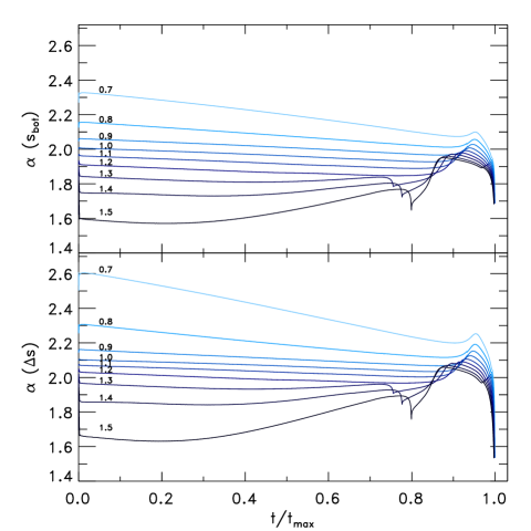
Figure 9: Mixing-length parameter along stellar evolutionary tracks with solar metallicity against the normalized age for the masses from 0.7 to 1.5 $M_{\odot}$ (indicated). The tracks are derived from the functional fits $f\left(T_{\mathrm{eff}},\log g\right)$ of $\alpha_{\mathrm{MLT}}$-calibrations with $s_{\mathrm{bot}}$ and $\Delta s$ (top and bottom panel, respectively) and all tracks end on the RGB when $\log g=1$.

The variation of $\alpha_{\mathrm{MLT}}$ along typical stellar evolutionary tracks ranges from $1.6$ to $2.4$ from higher to lower mass (see Fig. 9), and deviates by up to $\pm 20\,\%$ from the solar value ($\alpha_{\mathrm{MLT}}^{\odot}$). Note that in Fig. 9 we show $\alpha_{\mathrm{MLT}}$ along tracks calculated with a constant value of the mixing-length parameter ($1.78$) obtained from the usual solar model calibration (see Magic et al. 2010). The figure therefore does not show the actual, self-consistent changes in $\alpha_{\mathrm{MLT}}$ along the evolution, but, significant differences are hardly to be expected. During the main-sequence evolution $\alpha_{\mathrm{MLT}}$ varies only little and is almost constant, in particular for the lower masses without a convective core. The variable mixing-length parameter has a stronger influence during later evolutionary stages, the TO and the RGB ascent; $\alpha_{\mathrm{MLT}}$ increases first towards values around $\sim 1.9-2.1$, and then drops sharply to values of $\sim 1.7$ for all masses, which is the consequence of the narrow range in red giant temperature and surface gravity.

The mixing-length parameter not only determines $T_{\mathrm{eff}}$ of the stellar models, but also influences the adiabatic stratification of the 1D models in the deeper convection zone. In particular, for a larger $\alpha_{\mathrm{MLT}}$ the lower boundary of the convection zone is located deeper in the interior. Therefore, for stars with lower (higher) masses, a variable mixing-length parameter with stellar parameter will increase (decrease) the depth of the convection zone. As a consequence, one can expect that the convective mixing will be enhanced (reduced) for less (more) massive stars in stellar evolutionary calculations. This may influence, for example, the depletion and burning of Li in low-mass stars.

3.7 Comparison with observations

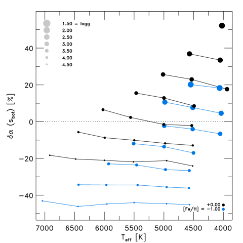
Figure 10: Relative differences between the the mixing-length parameter derived from observations and our 3D RHD models for different stellar parameters.

Observations provide an opportunity to constrain free parameters in theoretical models. Bonaca et al. (2012) attempted to calibrate the mixing-length parameter from Kepler-observations of dwarfs and subgiants (90 stars). Employing the usual scaling relations for the frequency of the maximal oscillation mode power, $\nu_{\mathrm{max}}$, and the large frequency separation, $\Delta\nu$ (see, for example, Huber et al. 2011), in connection with $T_{\mathrm{eff}}$ and $\left[\mathrm{Fe}/\mathrm{H}\right]$ from spectroscopic observations, they estimated mass and radius of the observed objects. From a grid of stellar evolutionary tracks computed with different $\alpha_{\mathrm{MLT}}$ values, they then selected the value that matched the inferred stellar parameters. The stellar evolutionary tracks were computed with the Yale stellar evolution code by employing the EOS and opacities from OPAL (see Demarque et al. 2008). For the outer boundary conditions they used the Eddington $T(\tau)$ relation and the standard MLT formulation by Böhm-Vitense (1958). These differences need be considered in the comparison of the resulting $\alpha_{\mathrm{MLT}}$ values.

Bonaca et al. (2012) derived an average mixing-length parameter of $1.60$ from the observations, which is in general lower than their solar-calibrated value with 1.69, which resulted from the 1D models without the comparison with observations. We compare the (linear) functional fit of $\alpha_{\mathrm{MLT}}$ derived in Bonaca et al. (2012), with stellar parameters to our own results in Fig. 10. We compare the calibration resulting from their complete data set. They also derived a fit for a subset of dwarfs, which is quite restricted in the range of stellar parameters and quite different from the fit for the full sample, however, they determined the solar mixing-length parameter with $\alpha_{\mathrm{MLT}}^{\odot}=1.59$, which is $20\,\%$ lower than our result of $1.98$. However, we remark that because of differences in the input physics and methods, the comparison between absolute values of $\alpha_{\mathrm{MLT}}$ is limited. Interestingly, the variation with $T_{\mathrm{eff}}$ for a given $\log g$ and $\left[\mathrm{Fe}/\mathrm{H}\right]$ is rather similar apart from an almost constant offset. For different $\log g$ and $\left[\mathrm{Fe}/\mathrm{H}\right]$, we find significant systematical differences (see Fig. 10). The values for dwarfs are in general lower by up to $\sim 20-40\,\%$ depending on gravity and metallicity, while the values for giants are greater by the similar amount. The comparison is made more difficult because even the full sample of Bonaca et al. (2012) is rather limited in $\log g$, and biased towards dwarfs. Additionally, the input physics (EOS and opacity) of their models deviates from ours. The authors themselves mention the absence of strong correlations with $\log g$, their restricted range in $\mathrm{[Fe/H]}$, the discrepancies to the results by Ludwig et al. (1999) and Trampedach (2007), and the fact that $\alpha_{\mathrm{MLT}}$ effectively compensates for everything else that influences $T_{\mathrm{eff}}$.

Our mixing-length parameters also differ significantly from the spectroscopical findings by Fuhrmann et al. (1993), who concluded that one would need an $\alpha_{\mathrm{MLT}}$ with very low values with $\sim 0.5$, to properly fit hydrogen lines for various stars with the resulting temperature stratifications. This, however, can be explained completely by the fact that here only the outermost convective layers are traced, which are not tested with our method for inferring $\alpha_{\mathrm{MLT}}$ from the adiabatic structure at the bottom of the convection zone, and that the mixing-length parameter is indeed depth-dependent (see Sect. 4.2). This was already verified by Schlattl et al. (1997).

4 Mass mixing-length parameter

4.1 Deriving the mass mixing-length parameter

In the following, we denote the temporal and spatial averaged thermodynamic quantities with $\left\langle\dots\right\rangle$, which depict only the $z$-dependence. Then, the momentum equation for a stationary system yields

$$\partial_{z}\left(\left\langle p_{\mathrm{th}}\right\rangle+\big{<}\rho v_{z}^{2}\big{>}\right) = \left\langle\rho\right\rangle g,$$

where the divergence of the viscosity stress tensor vanishes on average. This equation states that a given mass stratification ($\rho g$) has to be supported by the joint thermodynamic ($p_{\mathrm{th}}$) and turbulent pressure ($p_{\mathrm{turb}}=\rho v_{z}^{2}$) forces to sustain equilibrium. Since the vertical velocity, $v_{z}$, appears here, we solve for the latter and obtain

$$\left\langle v_{z}\right\rangle \simeq \sqrt{\frac{g-\left\langle p_{\mathrm{th}}\right\rangle/\left\langle\rho\right\rangle\partial_{z}\ln\left\langle p_{\mathrm{th}}\right\rangle}{\partial_{z}\ln\left\langle\rho\right\rangle+2\partial_{z}\ln\left\langle v_{z}\right\rangle}}.$$

Here, we assume that $\big{<}\rho v_{z}^{2}\big{>}=\left\langle\rho\right\rangle\left\langle v_{z}\right\rangle^{2}$, but, we validated this equation with comparisons of averaged models. Then, similar to the temperature gradient, $\@vec{\nabla}=d\ln\left\langle T\right\rangle/d\ln\left\langle p_{\mathrm{tot}}\right\rangle$, we introduce the notation for the gradient for a value $X$, but, instead of the total pressure it is scaled by the thermodynamic pressure scale height,

$$\nabla_{X} = \partial_{z}\ln\left\langle X\right\rangle/\partial_{z}\ln\left\langle p_{\mathrm{th}}\right\rangle,$$

and we can rewrite the vertical velocity to

$$\left\langle v_{z}\right\rangle \simeq \sqrt{\frac{g/\partial_{z}\ln\left\langle p_{\mathrm{th}}\right\rangle-\left\langle p_{\mathrm{th}}\right\rangle/\left\langle\rho\right\rangle}{\nabla_{\rho}+2\nabla_{v_{z}}}}.$$ (1)

This equation depicts the correlation of the vertical velocity with the gravity and pressure stratification, as well as the gradient of the density and the gradient of the vertical velocity itself in the hydrodynamic equilibrium. Now, we consider the gradient of the absolute vertical mass flux, $\left\langle j_{z}\right\rangle=\left\langle\rho v_{z}\right\rangle$, for the up- or downflows (because of conservation of mass, the mass flux of the upflows, $j_{z}^{\uparrow}$, equals the mass flux of the downflows, $j_{z}^{\downarrow}$) with

$$\nabla_{j_{z}} = \frac{\partial_{z}\ln|\big{<}j_{z}^{\mathrm{\uparrow\downarrow}}\big{>}|}{\partial_{z}\ln\left\langle p_{\mathrm{th}}\right\rangle},$$

which indicates the length over which the up- or downflow has changed by the $e$-fold, where the length scale is expressed in pressure scale heights. Trampedach & Stein (2011) introduced the mass mixing-length as the inverse vertical mass flux scale height, that is $l_{m}=\partial_{z}\ln|\big{<}j_{z}^{\mathrm{\uparrow\downarrow}}\big{>}|^{-1}$, which is in concordance with the gradient of the vertical mass flux with $l_{m}=H_{P}/\nabla_{j_{z}}$. Furthermore, we define the mass mixing-length parameter as the inverse gradient of the vertical mass flux,

$$\alpha_{m} \equiv \nabla_{j_{z}}^{-1},$$ (2)

and we can decompose the gradient of the vertical mass flux into its components and find

$$\alpha_{m} \simeq \left(\nabla_{\rho}+\nabla_{v_{z}}\right)^{-1},$$ (3)

which states that the mass mixing-length parameter is the inverse sum of the changes in the density and vertical velocity gradients. The gradient of the filling factor also contributes, but, since it vanishes in the deeper adiabatic convection zone and contributes only very little confined to the photospheric transition region, we nelgect this in our discussions (see Trampedach & Stein 2011). We note that the definition in Eq. 2 is the same as introduced by Trampedach & Stein (2011). Finally, we can now identify the mass mixing-length parameter in the denominator of the vertical velocity (Eq. 1) and obtain the following expression:

$$\left\langle v_{z}\right\rangle \simeq \sqrt{\frac{\alpha_{m}}{1+\alpha_{m}\nabla_{v_{z}}}\left(\frac{g}{\partial_{z}\ln\left\langle p_{\mathrm{th}}\right\rangle}-\frac{\left\langle p_{\mathrm{th}}\right\rangle}{\left\langle\rho\right\rangle}\right)}.$$ (4)

This illustrates why the vertical velocity depends on the mass mixing-length parameter, similarly to the MLT velocity $v_{\mathrm{MLT}}$, which depends on mixing-length parameter with $v_{\mathrm{MLT}}\propto\alpha_{\mathrm{MLT}}$ (see Eq. 9).

To complete the comparison of the mass mixing-length parameter with the (MLT) mixing-length parameter, we derive its dependence on the convective energy flux. We assume that the mean convective energy flux consists of the fluctuations of the total energy ($\varepsilon_{\mathrm{tot}}=\varepsilon+p_{\mathrm{th}}/\rho+\@vec{v}^{2}/2$), which we depicted with $f$, and is carried by the mean vertical mass flux, that is

$$\left\langle F_{\mathrm{conv}}\right\rangle \sim \left\langle f\right\rangle\left\langle\rho v_{z}\right\rangle,$$

where we assume that $v_{z}$ is the hydrodynamic velocity given in Eq. 1 and also that $\big{<}\rho v_{z}\big{>}=\left\langle\rho\right\rangle\left\langle v_{z}\right\rangle$. We determine the divergence of the convective energy flux, $\partial_{z}\left\langle F_{\mathrm{conv}}\right\rangle$, and solve for the total energy fluctuations, which yields

$$f \simeq \frac{1}{\nabla_{\rho}+\nabla_{v_{z}}}\frac{\partial_{z}\left\langle F_{\mathrm{conv}}\right\rangle/\left\langle\rho v_{z}\right\rangle+\partial_{z}\left\langle f\right\rangle}{\partial_{z}\ln\left\langle p_{\mathrm{th}}\right\rangle}.$$

Then, we can substitute the convective energy losses, $\partial_{z}\left\langle F_{\mathrm{conv}}\right\rangle$, by the radiative cooling rate, $-\left\langle q_{\mathrm{rad}}\right\rangle$, because of conservation of total energy, and we can identify the mass mixing-length parameter in the convective energy flux as well and obtain

$$\left\langle F_{\mathrm{conv}}\right\rangle \simeq -\alpha_{m}\frac{\left(\left\langle q_{\mathrm{rad}}\right\rangle+\left\langle\rho v_{z}\right\rangle\partial_{z}\left\langle f\right\rangle\right)}{\partial_{z}\ln\left\langle p_{\mathrm{th}}\right\rangle}.$$ (5)

This equation is basically the expression for the conservation of energy. These two equations for the velocity and the convective energy flux are just reformulated approximations of the hydrodynamic mean-field equations. To close this set of equations, one still would need information about the gradient of the velocity and total energy fluctuation, as well as the radiative cooling rates.

4.2 Depth-dependence of the mass mixing-length parameter

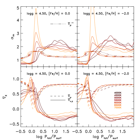
Figure 11: Top panel: The mass mixing-length parameter $\alpha_{m}$ from Eq. 3 (solid) and the inverse gradient of the density, $\nabla_{\rho}^{-1}$ (triple-dotted dashed line). For clarity we excluded values with $\nabla_{\rho}^{-1}>5/3$ just below the optical surface ($0<\log p_{\mathrm{tot}}/p_{\mathrm{surf}}<0.5$). Bottom panel: the gradient for density, $\nabla_{\rho}$, and vertical velocity, $\nabla_{v_{z}}$, (dashed and solid lines, respectively) for different stellar parameters.

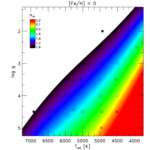
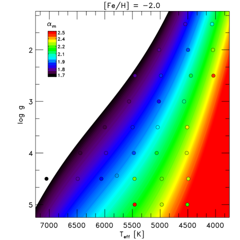
Figure 12: As Fig. 2, but here the mass mixing-length parameter $\alpha_{m}$ is shown.

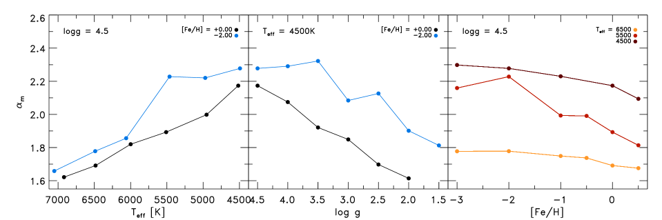
Figure 13: As Fig. 4, but here the mass mixing-length parameter $\alpha_{m}$ is shown.

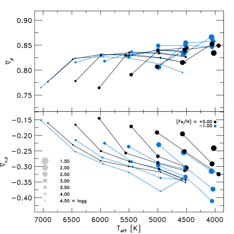
Figure 14: Mean gradient of the density, $\nabla_{\rho}$, and the vertical velocity, $\nabla_{v_{z}}$, in the convection zone for different stellar parameters.

Following Trampedach & Stein (2011), we tried to derive the mass mixing-length parameter from the vertical mass flux of the downflows (Eq. 2), but, we found that the fluctuations in the vertical velocity field are enhanced in our simulations, which is probably caused by the higher numerical vertical resolution (the simulations by Trampedach et al. 2013 have a thrice lower vertical resolution and therefore exhibit fewer turbulent and more laminar structures in the downflows). We found the rms vertical velocity to be less sensitive to the statistical fluctuations in the deeper convection zone, therefore, we derived the mass mixing-length by using the gradient of the rms vertical velocity in Eq. 3, instead of deriving the mass mixing-length from the vertical mass flux of the downflows (Eq. 2). Therefore, a comparison with Trampedach & Stein (2011) is only qualitatively meaningful.

In Fig. 11, we illustrate the horizontally and temporally averaged, depth-dependent mass mixing-length parameter for different stellar parameters, which we derived from our 3D RHD simulations. In the convection zone, the mass mixing-length parameter has values around $\sim 2$, while above the optical surface, $\alpha_{m}$ has lower values around $\sim 0.5$. Fuhrmann et al. (1993) found that similar low values for the mixing-length parameter $\alpha_{\mathrm{MLT}}$ yield better fits for Balmer lines, but, they also used high values for the temperature distribution parameter with $y=0.5$ (see also App. C.2), and moreover, the influence of $\alpha_{\mathrm{MLT}}$ becomes negligible towards the optical surface, where the Balmer lines form (see Fig. 1). Therefore, the agreement of the depth-dependent $\alpha_{m}$ with their low values for $\alpha_{\mathrm{MLT}}$ might be just a coincidence. Furthermore, just below the optical surface ($\log p_{\mathrm{tot}}/p_{\mathrm{surf}}=0$) at the photospheric transition region, $\alpha_{m}$ features a peak, which depends on the stellar parameters, in particular, for higher $T_{\mathrm{eff}}$, the peak in between increases, while in the convection zone it is the flatter. We remark that the peak in $\alpha_{m}$ coincides with the location of the peak in the $v_{z,\mathrm{rms}}$. We also included the inverse gradient of density in the same figure with $\alpha_{m}$, demonstrating that the adiabatic value of $\alpha_{m}$ in the convection zone is mainly contributed by the density gradient.

We also show the gradients of the density and vertical velocity in Fig. 11, which are the two main components of $\alpha_{m}$. The gradients of the filling factors also contribute to the variation of mass mixing-length. However, similar to the findings by Trampedach & Stein (2011), we find that the fillings factors are constant in the convection zone, therefore, their contribution is negligible. The variation of $\alpha_{m}$ in the convection zone arises mainly because of the different velocity gradients, since the density gradient converges always to very similar adiabatic values ($\gamma_{\mathrm{ad}}\simeq\nabla_{\rho}^{-1}$). For a monoatomic ideal gas with radiation pressure the adiabatic exponent is given by $\gamma_{\mathrm{ad}}=\left(1-\nabla_{\mathrm{ad}}\right)^{-1}$, and with $\nabla_{\mathrm{ad}}=1/4$ one obtains $\gamma_{\mathrm{ad}}\sim 4/3$ (Kippenhahn et al. 2013, see). $\nabla_{\rho}^{-1}$ it is close to 1.2 (see Fig. 11). For a nonideal gas differences due to nonideal effects are to be expected. On the other hand, $\nabla_{\rho}$ is close to $\sim 0.8$ therefore, similar to a value for an ideal gas with $3/4$, while $\nabla_{v_{z}}$ is between $-0.4$ and $-0.15$ (see also Fig. 14).

In the vicinity of the optical surface, the cooling rates are imprinted on the gradients for the density and velocity with a sharp transition. Towards the interior, the density increases because of the stratification and hydrostatic equilibrium, hence the gradient is $\nabla_{\rho}>0$, while the velocity decreases, and therefore $\nabla_{v_{z}}<0$. The signs of $\nabla_{\rho}$ and $\nabla_{v_{z}}$ are opposite because of the conservation of mass. In the interior, the stellar fluid is compressed and the velocity slows down, meaning that the convective energy is carried with a slower, thicker mass flux. For higher $T_{\mathrm{eff}}$, the (negative) velocity gradient has a lower amplitude and is therefore closer to zero, and a smaller amplitude of $\nabla_{v_{z}}$ implies a steeper drop of the vertical velocity towards the interior, which also entails a larger maximum of the vertical velocity (see Fig. 14). The velocity gradient reduces the density gradient, but, a lower sum of $\nabla_{\rho}$ and $\nabla_{v_{z}}$ relates to a higher $\alpha_{m}$ because of the inverse relation (see Fig. 12). Since the density gradient is very similar for different stellar parameters, the variation in $\alpha_{m}$ arises mainly from the differences in the velocity gradient. Therefore, we can relate the variation of the entropy jump with the variation of the velocity gradient, that is $\Delta s\sim e^{\nabla_{v_{z}}}$, which was also concluded by Trampedach & Stein (2011) for the mass mixing-length parameter in an extended solar simulation.

4.3 Mean mass mixing-length parameter in the convection zone

We determined the mean mass mixing-length parameter of the convection zone below the optical surface between the location of the peak in the density scale height, that is $\max\left(\partial_{z}\ln\rho\right)_{\tau>1}$, and the bottom, but, avoided bottom boundary effects on the vertical velocity. We performed linear fits of the density and vertical rms-velocity gradients by considering all snapshots, and from both gradients we determined the mean value of $\alpha_{m}$ as given in Eq. 3. We note that our method of retrieving a mean value differs from that by Trampedach & Stein (2011). The convection zones in the 3D simulations have to be extended enough, so that lower boundary effects on the vertical velocities are minimized, which is the case for most models, except for some metal-poor giants that are slightly too shallow to properly match $\alpha_{m}$.

The results for $\alpha_{m}$ are displayed in Fig. 12, while in Fig. 14 we depict the mean values of the density and velocity gradients. From the solar simulation we determined $\alpha_{m}^{\odot}=1.83$, which is close to the solar mass mixing-length parameter by Trampedach & Stein (2011) with $1.76$. Furthermore, the mass mixing-length parameter depicts qualitatively very similar systematic variations with stellar parameter, as we found for $\alpha_{\mathrm{MLT}}$ above. In particular, it decreases for higher $T_{\mathrm{eff}}$ and $\left[\mathrm{Fe}/\mathrm{H}\right]$, and lower $\log g$, and the range in $\alpha_{m}$ between $\sim 1.7$ and $\sim 2.3$ is qualitatively similar to that of $\alpha_{\mathrm{MLT}}$ (see also Fig. 13). In general, we find values for $\alpha_{m}$ that are qualitatively similar to those found by Trampedach & Stein (2011), in particular, the dwarf models ($\log g=4.5$) have a similar slope with $T_{\mathrm{eff}}$. As mentioned above, we consider the mass mixing-length parameter from the gradients of the density and rms vertical velocity (see Eq. 3) instead of the unidirectional mass flux, and we also used a different method for determining a mean value, therefore, differences in the results are to be expected.

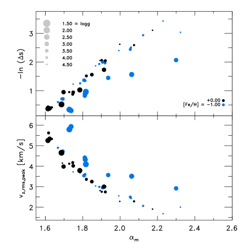
Figure 15: Correlation of the mass mixing-length parameter, $\alpha_{m}$, with the logarithmic inverse of the entropy jump $-\ln\left(\Delta s\right)$ and the peak of the vertical rms-velocity (top and bottom panel, respectively).

The variation of $\alpha_{m}$ is also similar to the logarithmic inverse variation of the entropy jump. In Fig. 15 we compare $\alpha_{m}$ with the logarithmic inverse entropy jump and find a similar tight correlation between the two as we found for the mixing-length parameter $\alpha_{\mathrm{MLT}}\left(\Delta s\right)$ above (Sect. 3.3). The stronger deviations for the metal-poor giants originate from the fact that these models are slightly shallower, therefore, the match of the mass mixing-length parameter is perturbed because of the lower boundary effects on the velocity. We also illustrate the tight anticorrelation of the peak vertical rms-velocity with the mass mixing-length parameter in Fig. 15.

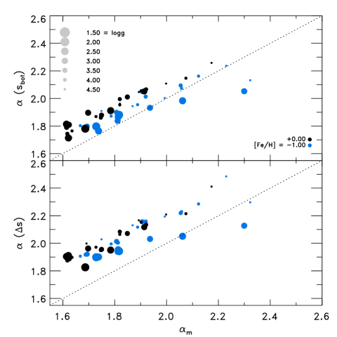
Figure 16: Comparison of the mass mixing-length parameter, $\alpha_{m}$, with the mixing-length parameter calibrated with $s_{\mathrm{bot}}$ and $\Delta s$ (top and bottom panel, respectively).

A comparison of the mass mixing-length parameter with the mixing-length parameter calibrated with the entropy of the deep adiabatic convection zone and the entropy jump is shown in Fig. 16, and these also correlate well. The mixing-length parameters are slightly higher than $\alpha_{m}$ with a systematic offset around $\sim 0.1$ and $\sim 0.2$, which smaller for $\alpha_{\mathrm{MLT}}\left(s_{\mathrm{bot}}\right)$ than for $\alpha_{\mathrm{MLT}}\left(\Delta s\right)$. This illustrates that the mixing-length parameter in the framework of MLT has a physical background that originates in the mass mixing-length parameter (or inverse vertical mass flux gradient). However, since the MLT is incomplete, a one-to-one correspondence between $\alpha_{\mathrm{MLT}}$ and $\alpha_{m}$ is hardly expected; nonetheless, the good agreement between the two is an interesting result.

5 Velocity correlation length

The physical interpretation of the mixing-length parameter is conceptually the mean free path of a convective eddy over which it can preserve its identity before it resolves into its environment. In a real stratified hydrodynamic fluid the spatial two-point (auto)correlation function of the vertical velocity can be regarded as the 3D analog of the mixing-length parameter $\alpha_{\mathrm{MLT}}$ as proposed by Chan & Sofia (1987). The two-point correlation function for the values $q_{1}$ and $q_{2}$ is given by

$$C\left[q_{1},q_{2}\right] = \frac{\left\langle q_{1}q_{2}\right\rangle-\left\langle q_{1}\right\rangle\left\langle q_{2}\right\rangle}{\sigma_{1}\sigma_{2}},$$ (6)

with $\sigma_{i}$ being the the standard deviation of $q_{i}$ and $\left\langle\dots\right\rangle$ is the spatial horizontal average. To derive the vertical correlation function of the convective velocity field, we considered the vertical component of the velocity field, $v_{z}$, of a single fixed layer $z_{0}$ and derived the correlation functions for all other layers $z_{i}$, i.e. $C\left[v_{z_{0}},v_{z_{i}}\right]$, which was performed for twenty equidistant layers and covered the whole vertical depth scale of the simulation box.

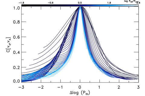
Figure 17: Vertical two-point correlation function of the vertical velocity, $C\left[v_{z},v_{z}\right]$, vs. the difference in the thermodynamic pressure, $\Delta\log P_{\mathrm{th}}$, for the solar simulation. The different heights are indicated with a blue color-coding. Note the convergence of the correlation width in the convection zone against an adiabatic value.

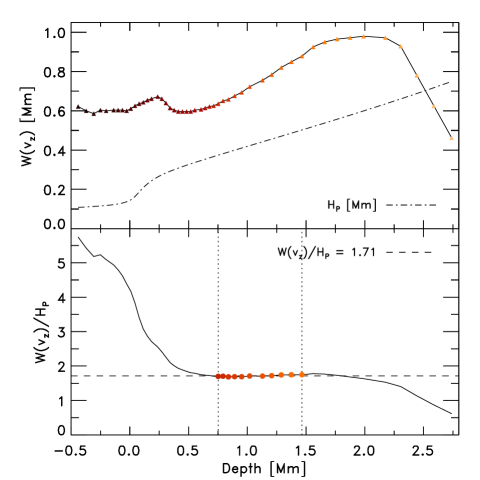
Figure 18: Top panel: Vertical correlation length of the vertical velocity (solid line with triangles) and pressure scale height (dotted-dashed line) shown against the depth for the solar model. We indicate the different heights with the same color-coding as used in Fig. 17. Bottom panel: Vertical correlation length scaled by the pressure scale height, which yields an average of $1.71$ (dashed line) in the considered region for averaging the correlation length (vertical dotted lines with filled circles) for the solar simulation.

In Fig. 17 we show the two-point correlation function of the vertical velocity field, $C\left[v_{z},v_{z}\right]$, derived for the solar simulation for the individual snapshots and then temporally averaged. For convenience, the correlation function is shown in differences of logarithmic pressure to the considered layer, $\Delta\log P_{\mathrm{th}}=\log P_{\mathrm{th}}(z_{0})-\log P_{\mathrm{th}}(z_{i})$. Then, the correlation function always reaches unity for $z_{i}=z_{0}$ and has a Gaussian-like shape. Furthermore, it is broader above the optical surface ($p_{\mathrm{tot}}/p_{\mathrm{surf}}=1$), which is due to the rapid decline of the pressure scale height; while below the latter the width seems to converge on a certain adiabatic value (see Fig. 18). When one considers the width of the correlation function in geometrical depth, instead of pressure, then $W\left(v_{z}\right)$ is constant around $\sim 0.6\,\mathrm{Mm}$ from the top down to $\sim 0.5\,\mathrm{Mm}$ and increases then with a fixed multiple ($1.71$) of the pressure scale height (see Fig. 18), which is the same as Robinson et al. (2003) found. The higher values for $W\left(v_{z}\right)/H_{P}$ above $0.5\,\mathrm{Mm}$ result from the lower $H_{P}$.

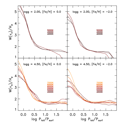
Figure 19: Correlation length of the vertical velocity vs. surface normalized pressure for different stellar parameters.

The full-width at half maximum (FWHM) of the two-point correlation function of the vertical velocity, $C\left[v_{z},v_{z}\right]$, which we denote with $W\left(v_{z}\right)$, gives an estimate on the size or length scale of the coherent vertical structures. The characteristic local length scale for the turbulent convective eddies can be determined with $W\left(v_{z}\right)$. With the term vertical correlation length we refer to $W\left(v_{z}\right)$. Similar to the mixing-length, it is preferable to scale the correlation length by the pressure scale height, that is $W\left(v_{z}\right)/H_{P}$, since the the latter increases towards deeper layers. Then, for the solar simulation (see Fig. 18) the converging value for the width is $W\left(v_{z}\right)/H_{P}=1.71$. This means that the coherent vertical structures extend $1.71H_{P}$ in the convection zone, and this value is similar to the mixing-length parameter ($\alpha_{\mathrm{MLT}}=1.94$). Chan & Sofia (1987, 1989) also found a similar scaling of $C\left[v_{z},v_{z}\right]$ with pressure scale height in a 3D simulation for the Sun. For different stellar parameters we find a rather similar convergence of the correlation length of the vertical velocity in the convection zone (see Fig. 19). Ludwig et al. (2006) found similar values for the correlation length of the vertical velocity with $W\left(v_{z}\right)/H_{P}\sim 2$ in the vicinity of the lower boundary for a number of different simulations, while Viallet et al. (2013) recently found for a red-giant simulation that the vertical correlation length of the vertical velocity scales with approximately twice of the pressure scale height.

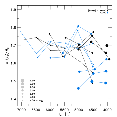
Figure 20: Overview of mean vertical correlation length of the vertical velocity in the convection zone for different stellar parameters.

We also determined the mean value of the correlation length in the convection zone below $\log p_{\mathrm{tot}}/\log p_{\mathrm{surf}}>1$. Close to the bottom boundary, the correlation function will increasingly overturn because we lack information in the deeper layers. Therefore, we applied for a mean correlation length a cut at the bottom, where $W\left(v_{z}\right)/H_{P}$ begins to decrease (see Fig. 18).

The resulting mean values of $W\left(v_{z}\right)/H_{P}$ for different stellar parameters are depicted in Fig. 20. They are distributed between $\sim 1.5$ and $\sim 1.8$. This is an interesting result, since it confirms, to a certain extent, the physical motivation for the mixing-length parameter, $\alpha_{\mathrm{MLT}}$: the vertical velocity field, hence the vertical mass flux, correlates similarly with the pressure scale heights in the convection zone. However, the variation of $W\left(v_{z}\right)/H_{P}$ with stellar parameters (Fig. 20) is not as clear and systematical as we found above for $\alpha_{\mathrm{MLT}}$ and $\alpha_{m}$ (see Sect. 4).

Furthermore, in contrast to the mixing-length parameter ($\alpha_{\mathrm{MLT}}$ and $\alpha_{m}$), the correlation length seems to increase for higher $T_{\mathrm{eff}}$. The reason for this might be the horizontal granule size, which we found to decrease slightly for lower effective temperatures, since the pressure scale height decreases (see Paper I). Moreover, the granular cells, which can be highlighted with the temperature excess from the background, feature distinct regular flat cylindric or pillar-like topologies.

Finally, we considered the correlation length of other variables and found that the horizontal velocity is rather similar, but with slightly lower correlation length with $\sim 1.4$. In addition, the entropy, temperature, and pressure have values around $\sim 1.3$, while the value for the density is close to unity.

6 Conclusions

We have calibrated the mixing-length parameter using realistic 3D RHD simulations of stellar surface convection by employing a 1D MLT stellar atmosphere code with identical microphysics. The calibration was achieved by varying the mixing-length parameter and matching the adiabatic entropy value of the deeper convection zone, $s_{\mathrm{bot}}$, or alternatively, matching the entropy jump, $\Delta s$. In both ways we found the mixing-length to decrease for higher $T_{\mathrm{eff}}$ and $\left[\mathrm{Fe}/\mathrm{H}\right]$, and lower $\log g$. The mixing-length varies in the range of $1.7-2.3$ for $\alpha_{\mathrm{MLT}}\left(s_{\mathrm{bot}}\right)$ and $\sim 1.8-2.4$ for $\alpha_{\mathrm{MLT}}\left(\Delta s\right)$, and will lead to differences of up to $\pm 20\,\%$ in $\alpha_{\mathrm{MLT}}$ depending on the stellar mass. This changes the stellar interior structure by extending or shortening the depth of the convection zone and thus the stellar evolution; we intend to investigate in future studies how in detail a realistic $\alpha_{\mathrm{MLT}}$ will impact basic stellar evolution predictions.

Furthermore, we derived from the hydrodynamic mean field equations (for the first-time) a physically motivated connection of the mass mixing-length, which is the inverse of the vertical mass flux gradient, with the mixing-length. We determined the mass mixing-length parameter and found that it varies qualitatively similar to the mixing-length parameter in the range of $1.6-2.3$. The mass mixing-length parameter is also depth-dependent and decreases above the surface to lower values around $\sim 0.5$, which agrees with previous findings from observations. Finally, the mass mixing-length parameter and mixing-length parameter strongly correlate with the logarithmic inverse of the entropy jump for different stellar parameters, that is $\alpha_{\mathrm{MLT}}\sim-\ln\Delta s$. Finally, we also derived the vertical velocity correlation length, which features values similar to that of the mixing-length with approximately $\sim 1.6-1.8$ of pressure scale height, but, the dependence with $T_{\mathrm{eff}}$ is inverted, meaning that the correlation length decreases with $T_{\mathrm{eff}}$.

To summarize the importance of our work: we can finally remove the free parameters inherent in MLT and also avoid having to use solar calibrations for other stars.

Appendix A Tables

In Table 1, we list results for the solar metallicity. The complete table is available at CDS cdsarc.u-strasbg.fr and also at www.stagger-stars.net.

Table 1: Stellar parameters: effective temperature, $T_{\mathrm{eff}}$, and surface gravity, $\log g$ (Cols. 1 and 2 in $\left[\mathrm{K}\right]$ and $\left[\mathrm{dex}\right]$).

$T_{\rm{eff}}$	$\log g$	$\lg\rho_{\mathrm{bot}}$	$\lg T_{\mathrm{bot}}$	$\lg p_{\mathrm{th}}^{\mathrm{bot}}$	$s_{\mathrm{bot}}$	$\Delta s$	$\delta s_{\mathrm{rms}}^{\mathrm{peak}}$	$\delta\rho_{\mathrm{rms}}^{\mathrm{peak}}$	$\delta v_{z,\mathrm{rms}}^{\mathrm{peak}}$	$\alpha_{\mathrm{MLT}}^{s_{\mathrm{bot}}}$	$\alpha_{\mathrm{MLT}}^{\Delta s}$	$\alpha_{m}$	$W(v_{z})/H_{P}$
4023	1.50	0.717	4.272	1.061	2.304	0.594	14.023	46.897	0.465	1.781	1.826	1.686	1.698
4052	2.00	1.125	4.233	1.368	2.018	0.359	9.088	35.288	0.379	1.912	1.951	1.784	1.658
3938	2.50	1.691	4.239	1.889	1.776	0.177	4.733	24.764	0.300	2.051	2.117	1.914	1.621
4569	2.00	0.679	4.342	1.120	2.417	0.692	16.099	50.583	0.525	1.814	1.904	1.614	1.719
4532	2.50	1.357	4.279	1.669	2.039	0.387	9.935	36.301	0.398	1.896	1.962	1.697	1.753
4492	3.00	1.785	4.266	2.029	1.808	0.211	5.783	26.808	0.325	2.011	2.071	1.849	1.775
4530	3.50	2.103	4.269	2.322	1.682	0.129	3.707	20.261	0.274	2.066	2.135	1.921	1.656
4513	4.00	2.419	4.277	2.625	1.580	0.075	2.205	14.454	0.229	2.147	2.215	2.075	1.487
4516	4.50	2.721	4.292	2.927	1.503	0.045	1.348	9.928	0.191	2.258	2.411	2.173	1.546
4512	5.00	3.013	4.308	3.226	1.436	0.029	0.830	6.377	0.154	2.342	2.907	2.221	1.684
4932	2.00	0.042	4.535	0.700	2.766	0.948	21.258	69.923	0.725	1.714	1.911	1.621	1.630
5013	2.50	0.883	4.374	1.358	2.381	0.683	16.250	51.278	0.534	1.809	1.890	1.623	1.676
4998	3.00	1.534	4.308	1.882	2.026	0.390	10.116	35.942	0.402	1.879	1.956	1.749	1.705
5001	3.50	1.960	4.295	2.243	1.805	0.220	6.134	27.035	0.336	1.995	2.084	1.820	1.698
4978	4.00	2.292	4.293	2.538	1.662	0.126	3.700	19.745	0.275	2.056	2.153	1.902	1.687
4953	4.50	2.604	4.301	2.837	1.561	0.073	2.196	14.015	0.228	2.108	2.209	1.998	1.607
4963	5.00	2.885	4.314	3.118	1.487	0.045	1.398	9.888	0.185	2.143	2.227	2.130	1.577
5465	3.00	1.084	4.403	1.589	2.343	0.657	15.917	48.856	0.527	1.791	1.893	1.614	1.742
5560	3.50	1.663	4.345	2.062	2.043	0.417	10.870	37.436	0.418	1.861	1.951	1.747	1.637
5497	4.00	2.139	4.322	2.456	1.791	0.221	6.244	26.379	0.333	1.953	2.065	1.820	1.684
5510	4.50	2.486	4.322	2.769	1.649	0.128	3.791	19.527	0.281	2.047	2.167	1.893	1.668
5480	5.00	2.791	4.330	3.060	1.548	0.076	2.343	14.272	0.225	2.068	2.186	2.002	1.670
5768	4.44	2.367	4.336	2.688	1.725	0.184	5.313	23.788	0.308	1.979	2.089	1.825	1.702
6023	3.50	1.130	4.493	1.737	2.403	0.715	17.022	51.883	0.562	1.744	1.875	1.617	1.764
5993	4.00	1.865	4.364	2.281	1.994	0.387	10.302	35.917	0.412	1.869	1.971	1.728	1.700
5998	4.50	2.301	4.344	2.644	1.771	0.218	6.225	25.994	0.332	1.962	2.081	1.820	1.670
6437	4.00	1.384	4.495	1.989	2.322	0.659	16.117	48.227	0.533	1.765	1.898	1.635	1.739
6483	4.50	2.008	4.386	2.448	1.972	0.378	10.054	34.007	0.415	1.889	1.998	1.691	1.744
6918	4.50	1.545	4.543	2.201	2.301	0.652	15.738	46.039	0.526	1.796	1.911	1.621	1.730

Notes: The conditions at the lower boundary: density, $\rho$, temperature, $T$, pressure, $p_{\mathrm{th}}$, entropy at the bottom; the entropy jump, $\Delta s$; the peak fluctuations in: entropy, $\delta s_{\mathrm{rms}}^{\mathrm{peak}}$, density, $\delta\rho_{\mathrm{rms}}^{\mathrm{peak}}$, vertical velocity $v_{z,\mathrm{rms}}^{\mathrm{peak}}$; the mixing-length: $\alpha_{\mathrm{MLT}}\left(s_{\mathrm{bot}}\right)$ and $\alpha_{\mathrm{MLT}}\left(\Delta s\right)$; mass mixing-length parameter, $\alpha_{m}$, and correlation length $W\left(v_{z}\right)/H_{P}$.

Appendix B Functional fits

Similar to Ludwig et al. (1999), we performed functional fits of the mixing-length parameters and the mass mixing-length parameter with the $T_{\mathrm{eff}}$ and $\log g$ for the different metallicities individually. We transformed the stellar parameters with $x=(T_{\mathrm{eff}}-5777)/1000$ and $y=\log g-4.44$, and fitted the values with a least-squares minimization method for the functional basis

$$f\left(x,y\right) = a_{0}+\left(a_{1}+\left(a_{3}+a_{5}x+a_{6}y\right)x+a_{4}y\right)x+a_{2}y.$$ (7)

The resulting coefficients, $a_{i}$, are listed in Table 2.

Table 2: Coefficients $a_{i}$ of the linear function $f$ (Eq. 7) for $\alpha_{\mathrm{MLT}}\left(s_{\mathrm{bot}}\right)$, $\alpha_{\mathrm{MLT}}\left(\Delta s\right)$, and $\alpha_{m}$ for different metallicities. In the last two rows, we list the root-mean-square and maximal deviation of the fits.

Value	$\left[\mathrm{Fe}/\mathrm{H}\right]$	$a_{0}$	$a_{1}$	$a_{2}$	$a_{3}$	$a_{4}$	$a_{5}$	$a_{6}$	rms$\Delta$	max$\Delta$
$\alpha_{\mathrm{MLT}}(s_{\mathrm{bot}})$	+0.5	1.973739	-0.134290	0.163201	0.032132	0.046759	-0.025605	0.052871	0.022	0.040
	+0.0	1.976078	-0.110071	0.175605	0.003978	0.103336	-0.058691	0.080557	0.017	0.038
	-0.5	1.956357	-0.133645	0.133825	0.027491	0.049125	-0.048045	0.057956	0.027	0.042
	-1.0	1.969945	-0.143710	0.149004	0.001154	0.052837	-0.033471	0.037823	0.020	0.058
	-2.0	2.010997	0.012308	0.160894	-0.041272	0.180486	-0.059577	0.074409	0.033	0.067
	-3.0	2.133974	0.053307	0.222283	-0.192920	0.225412	-0.064937	0.027230	0.066	0.149
$\alpha_{\mathrm{MLT}}(\Delta s)$	+0.5	2.060065	-0.075697	0.183750	0.018061	0.160931	-0.110880	0.164789	0.063	0.091
	+0.0	2.077069	-0.079283	0.153376	0.041062	0.098795	-0.108972	0.137377	0.075	0.139
	-0.5	2.080653	-0.117156	0.139250	0.105874	0.063015	-0.104596	0.143233	0.095	0.206
	-1.0	2.131896	-0.135578	0.195694	0.039771	0.109232	-0.074565	0.110530	0.054	0.096
	-2.0	2.229049	-0.068633	0.248141	-0.043729	0.229523	-0.088846	0.112805	0.056	0.136
	-3.0	2.324527	-0.011662	0.293515	-0.171136	0.305021	-0.112595	0.077837	0.109	0.248
$\alpha_{m}$	+0.5	1.791089	-0.183788	0.179118	-0.022163	0.096536	-0.028233	0.054834	0.039	0.077
	+0.0	1.832344	-0.177105	0.166634	0.011835	-0.002416	-0.030472	0.019225	0.023	0.045
	-0.5	1.859980	-0.208802	0.154482	0.111923	-0.001357	-0.089213	0.105822	0.518	0.187
	-1.0	1.897928	-0.208284	0.174666	0.035389	0.020293	-0.045907	0.031081	0.133	0.123
	-2.0	1.959977	-0.255688	0.183739	0.032684	0.000570	-0.032134	0.000400	0.107	0.317

Appendix C Addendum on MLT

C.1 mixing-length formulation

In the framework of MLT, the convective flux is determined by

$$F_{\mathrm{conv}} = \left[\alpha_{\mathrm{MLT}}c_{P}T\Delta/2\right]\rho v_{\mathrm{MLT}},$$ (8)

with $c_{P}$ being the heat capacity, $\Delta$ the superadiabatic energy excess, and $\alpha_{\mathrm{MLT}}$ the adjustable mixing-length parameter, giving the mean free path of convective elements in units of pressure scale height. The convective velocity is determined by

$$v_{\mathrm{MLT}} = \sqrt{\alpha_{\mathrm{MLT}}^{2}gH_{P}\delta\Delta/\nu},$$ (9)

where $H_{P}$ is the pressure scale height, $\delta=-\left(\partial\ln\rho/\partial\ln T\right)_{p}$ the thermal expansion coefficient, and $\nu$ the energy dissipation by turbulent viscosity. The superadiabatic excess is given by

$$\Delta = \frac{\Gamma}{\left(1+\Gamma\right)}\left(\nabla-\nabla_{\mathrm{ad}}\right),$$ (10)

and the convective efficiency factor by

$$\Gamma = \frac{c_{P}}{8\sigma T^{3}}\tau_{e}\left(y+\tau_{e}^{-2}\right)\rho v_{\mathrm{MLT}},$$ (11)

with the optical thickness $\tau_{e}$, and temperature distribution $y$ of the convective element. The turbulent pressure

$$p_{\mathrm{turb}} = \beta\rho v_{\mathrm{turb}}^{2},$$ (12)

can be included, but a depth-independent turbulent velocity, $v_{\mathrm{turb}}$ is assumed, which is the common approach for atmospheric modeling. The resulting photospheric temperature stratifications are very similar to the MARCS (Gustafsson et al. 2008) and ATLAS models (Kurucz 1979; Castelli & Kurucz 2004). In Paper I, we showed that below the surface, where convective energy transport starts to dominate, the 1D models are systematically cooler than the $\left\langle\mathrm{3D}\right\rangle$ stratifications because of the fixed $\alpha_{\mathrm{MLT}}$ with $1.5$, in particular for hotter $T_{\mathrm{eff}}$.

C.2 Influence of additional MLT parameters

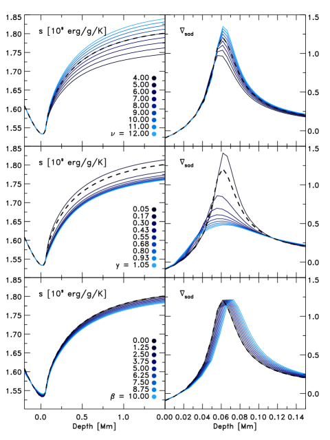
Figure 21: Entropy and superadiabatic gradient vs. depth (left and right panel, respectively) illustrating the influence of the additional MLT parameters $\nu$, $y$, and $\beta$ (top, middle, and bottom panel, respectively), the latter with the depth-independent $v_{\mathrm{turb}}=1\,\mathrm{km}/\mathrm{s}$. The mixing-length is kept fixed at $\alpha_{\mathrm{MLT}}=1.5$. We also included the standard values of $\beta=0$, $\nu=8$ and $y=0.076$ (dashed lines). Shown is the case for solar parameters.

In the formulation of Henyey et al. (1965) of MLT, there are at least three additional free parameters apart from $\alpha_{\mathrm{MLT}}$, which usually are not mentioned explicitly, but are compensated for by the value of $\alpha_{\mathrm{MLT}}$. These are the scaling factor of the turbulent pressure, $\beta$, the energy dissipation by turbulent viscosity, $\nu$, and the temperature distribution of a convective element, $y$. The default values are usually $\beta=1/2$, $\nu=8$ and $y=3/4\pi^{2}=0.076$ (see Gustafsson et al. 2008). In many cases, the turbulent pressure is neglected ($\beta=0$). In the notation of Ludwig et al. (1999), these parameters would yield $f_{1}=\nu^{-1}$ and $f_{4}=y^{-1}$, $f_{2}=1/2$ and $f_{3}=8/y$.

The turbulent pressure indirectly influences the $T$-stratification, gradients, and hydrostatic equilibrium by reducing the gas pressure. The parameter $\nu$ enters the convective velocity inverse proportionally, $v_{\mathrm{MLT}}\propto\nu^{-1}$ (see Eq. 9), and since $v_{\mathrm{MLT}}\propto\alpha_{\mathrm{MLT}}^{2}$, an increase in $\nu$ would have the same effect as a reduction in $\alpha_{\mathrm{MLT}}$, i.e. $\nu\propto s_{\mathrm{bot}}$. On the other hand, $y$ enters in the (nonlinear) convective efficiency factor, $\Gamma$, for the superadiabatic excess (see Eq. 11), and therefore $y$ is correlated with $\alpha_{\mathrm{MLT}}$ in a more complex way.

Considering a variation of the three additional parameters in the computation of the solar 1D model, we notice that the adiabatic entropy value of the deep convection zone is altered significantly (see Fig. 21). Furthermore, the two parameters $\nu$ and $y$ also change the entropy jump and the superadiabatic temperature gradient, $\@vec{\nabla}_{\mathrm{sad}}$, and in particular, its maximum of $\@vec{\nabla}_{\mathrm{sad}}$. The effect of the variation of $y$ on the entropy stratification is similar to that by $\alpha_{\mathrm{MLT}}$ (see Fig. 1). However, the entropy of the deep convection zone exhibits a more nonlinear dependence with the $y$ parameter. The increasing turbulent pressure with higher $\beta$ changes the stratification only slightly, but shifts the location of the maximum of $\@vec{\nabla}_{\mathrm{sad}}$ to the deeper interior. Towards the optical surface the influence of the MLT parameters decreases, as expected because of decreasing convective flux. A fine-tuning of $\beta$, $\nu$ and $y$ is only useful when these parameters introduce an independent influence on the mixing-length, since otherwise its effects can be summarized in $\alpha_{\mathrm{MLT}}$ alone.