Proposal for a Correction to the Temporal Correlation Coefficient Calculation for Temporal Networks

Abstract

Measuring the topological overlap of two graphs becomes important when assessing the changes between temporally adjacent graphs in a time-evolving network. Current methods depend on the fraction of nodes that have persisting edges. This breaks down when there are nodes with no edges, persisting or otherwise. The following outlines a proposed correction to ensure that correlation metrics have the expected behavior.

1 Previous Proposal

[1] defines the topological overlap in the neighborhood of $i$ between two consecutive time steps $[t_{m},t_{m+1}]$ as:

$$C_{i}(t_{m},t_{m+1})=\frac{\sum_{j}a_{ij}(t_{m})a_{ij}(t_{m+1})}{\sqrt{[\sum_{j}a_{ij}(t_{m})][\sum_{j}a_{ij}(t_{m+1})]}}$$ (1)

where $a_{ij}$ represents an entry in the unweighted adjacency matrix of the graph, so summing over $a_{ij}$ gives the interactions between $i$ and every other node.

Then the average topological overlap of the neighborhood of node $i$ as the average of $C_{i}(t_{m},t_{m+1})$ over all possible subsequent temporal snapshots:

$$C_{i}=\frac{1}{M-1}\sum_{m=1}^{M-1}C_{i}(t_{m},t_{m+1})$$ (2)

The average topological overlap of all $C_{i}$ can be said to represent the temporal clustering of all of the edges in the network, which we will call the temporal clustering coefficient (TCC).

$$C=\frac{1}{N}\sum_{i=1}^{N}C_{i}$$ (3)

Identically, the order of summations in this formulation can be reversed (simply to make the following more obvious), to give the average topological overlap of the graph at $t_{m}$ with the subsequent graph at $t_{m+1}$:

$$C_{m}=\frac{1}{N}\sum_{i=1}^{N}C_{i}(t_{m},t_{m+1})$$ (4)

and the same C is then given by:

$$C=\frac{1}{M-1}\sum_{m=1}^{M-1}C_{m}$$ (5)

According to [1] this formulation gives $C_{m}=1$ if and only if the graphs at $t_{m}$ and $t_{m+1}$ have exactly the same configuration of edges, and $C_{m}=0$ if the graph at $t_{m}$ and $t_{m+1}$ do not share any edges. This claim is only true if all of the $N$ nodes considered in the calculation have at least one edge.

Equation (1) results in an undefined $\frac{0}{0}$ in the case where the node $i$ has no edges in one or both time steps $t_{m}$ or $t_{m+1}$. If that undefined value is simply set to zero (choose zero because the node $i_{m}$ shares no edges with the node $i_{m+1}$), $C$ between identical unconnected graphs is equal to the fraction of connected nodes in the graph. The formula by [1] provides no method for dealing with networks where $N(t_{m})$ (the number of nodes participating in the network) changes in time.

This presents a significant problem, because for small time snapshots, many temporal graphs are often unconnected (contain unconnected nodes) [1] and $N(t_{m})$ changes constantly with time. For unconnected graphs, $C_{m}$ describing the relationship between two identical graphs gives $C_{m}\neq 1$, and can significantly underestimate the correlation between two graphs.

2 Proposed Correction

To ensure that $C_{m}$ has the expected behavior when the graph is unconnected, a constant $n$ is replaced by the maximum number of connected nodes in the network for the two time steps being compared. Using $\max[N(t_{m}),N(t_{m+1})]$ rather than simply $N(t_{m})$ or $N(t_{m+1}$ ensures that $C<1$ for all non-identical graphs, using $\min[N(t_{m}),N(t_{m+1})]$ would give $C=1$ for disconnected graphs where the only change is an edge appearing or disappearing. Be aware that this method will still give a $\frac{0}{0}$ for correlation between two graphs both with zero edges.

$$C_{m}=\frac{1}{\max[N(t_{m}),N(t_{m+1})]}\sum_{i=1}^{N}C_{i}(t_{m},t_{m+1})$$ (6)

$$C=\frac{1}{M-1}\sum_{m=1}^{M-1}\left(\frac{1}{\max[N(t_{m}),N(t_{m+1})]}\sum_{i=1}^{N}C_{i}(t_{m},t_{m+1})\right)$$ (7)

3 Examples

Below are some simple examples to show the difference between the two methods.

3.1 Connected graph

Figure 1: A connected graph. Here Methods 1 and 2 give the same result.

topological overlap in the neighborhood of $i$ between two consecutive time steps:

$$\text{(\ref{eq:Ci}): }C_{i}(t_{m},t_{m+1}):C_{i=1}(t_{m},t_{m+1})=\frac{1}{\sqrt{2}},\;C_{i=2}(t_{m},t_{m+1})=\frac{1}{\sqrt{2}},\;C_{i=3}(t_{m},t_{m+1})=0$$

Method 1: $C=\frac{1}{N}\sum_{i=1}^{N}\left(\frac{1}{M-1}\sum_{m=1}^{M-1}C_{i}(t_{m},t_{m+1})\right)=\frac{1}{3}\left(\frac{1}{1}(\frac{1}{\sqrt{2}}+\frac{1}{\sqrt{2}}+0)\right)=\frac{\sqrt{2}}{3}$

Method 2: $C=\frac{1}{M-1}\sum_{m=1}^{M-1}\left(\frac{1}{\max[N(t_{m}),N(t_{m+1})]}\sum_{i=1}^{N}C_{i}(t_{m},t_{m+1})\right)=\frac{1}{1}\left(\frac{1}{3}(\frac{1}{\sqrt{2}}+\frac{1}{\sqrt{2}}+0)\right)=\frac{\sqrt{2}}{3}$

3.2 Unconnected graph

Figure 2: An unconnected graph. As the graphs are identical the expected value is one, but method 1 for calculating $C$ gives $\frac{2}{3}$, or the fraction of nodes that are participating in the network at time $t_{m}$.

topological overlap in the neighborhood of $i$ between two consecutive time steps:

$$\text{(\ref{eq:Ci}): }C_{i}(t_{m},t_{m+1}):C_{i=1}(t_{m},t_{m+1})=1,\;C_{i=2}(t_{m},t_{m+1})=1,\;C_{i=3}(t_{m},t_{m+1})=\frac{0}{0}=0$$

Method 1: $C=\frac{1}{N}\sum_{i=1}^{N}\left(\frac{1}{M-1}\sum_{m=1}^{M-1}C_{i}(t_{m},t_{m+1})\right)=\frac{1}{3}(\frac{1}{1}(1+1+0))=\frac{2}{3}$

Method 2: $C=\frac{1}{M-1}\sum_{m=1}^{M-1}\left(\frac{1}{\max[N(t_{m}),N(t_{m+1})]}\sum_{i=1}^{N}C_{i}(t_{m},t_{m+1})\right)=\frac{1}{1}\left(\frac{1}{2}(1+1+0)\right)=1$

3.3 Time series with unconnected graphs

Figure 3: A network containing four nodes ($N=4$) which becomes disconnected during the observed time window ($N(t_{m})=4$, however, $N(t_{m+1})=3$ and $N(t_{m+2})=2$). Note three time steps, so $M=3$.

(1): $C_{i}(t_{m},t_{m+1})$:	$C_{i}(t_{m+1},t_{m+2})$:
$C_{i=1}(t_{m},t_{m+1})=\frac{2}{\sqrt{6}}$	$C_{i=1}(t_{m+1},t_{m+2})=\frac{1}{\sqrt{2}}$
$C_{i=2}(t_{m},t_{m+1})=1$	$C_{i=2}(t_{m+1},t_{m+2})=1$
$C_{i=3}(t_{m},t_{m+1})=1$	$C_{i=3}(t_{m+1},t_{m+2})=\frac{0}{0}=0$
$C_{i=4}(t_{m},t_{m+1})=\frac{0}{0}=0$	$C_{i=4}(t_{m+1},t_{m+2})=\frac{0}{0}=0$

Table 1: topological overlap in the neighborhood of $i$ between two consecutive time steps

Method 1:
(4): $C_{m}=\frac{1}{N}\sum_{i=1}^{N}C_{i}(t_{m},t_{m+1})$	(5): $C=\frac{1}{M-1}\sum_{m}^{M-1}C_{m}$
$C_{m}=\frac{1}{4}\sum_{i=1}^{4}C_{i}(t_{m},t_{m+1})\approx 0.70$	$\frac{1}{4}\sum_{m}^{3-1}C_{m}$
$C_{m+1}=\frac{1}{4}\sum_{i=1}^{4}C_{i}(t_{m+1},t_{m+2})\approx 0.45$	$\approx 0.57$

Method 2:
(6): $C_{m}=\frac{1}{\max[N(t_{m}),N(t_{m+1})]}\sum_{i=1}^{N}C_{i}(t_{m},t_{m+1})$	(7): $C=\frac{1}{M-1}\sum_{m}^{M-1}C_{m}$
$C_{m}=\frac{1}{4}\sum_{i=1}^{4}C_{i}(t_{m},t_{m+1})\approx 0.70$	$\frac{1}{3-1}\sum_{m}^{3-1}C_{m}$
$C_{m+1}=\frac{1}{3}\sum_{i=1}^{4}C_{i}(t_{m+1},t_{m+2})\approx 0.57$	$\approx 0.64$

3.4 Time series with identical unconnected graphs

Figure 4: A graph which becomes unconnected during the observed time window. Note that even though the second two time steps are identical, the $C$ between $t_{m}$ and $t_{m+1}$ $\neq 1$ because the graph is disconnected. Because of this, $C$ for the time series of graphs is underestimated when performing the calculation using Method 1.

(1): $C_{i}(t_{m},t_{m+1})$:	$C_{i}(t_{m+1},t_{m+2})$:
$C_{i=1}(t_{m},t_{m+1})=\frac{2}{\sqrt{6}}$	$C_{i=1}(t_{m+1},t_{m+2})=1$
$C_{i=2}(t_{m},t_{m+1})=1$	$C_{i=2}(t_{m+1},t_{m+2})=1$
$C_{i=3}(t_{m},t_{m+1})=1$	$C_{i=3}(t_{m+1},t_{m+2})=1$
$C_{i=4}(t_{m},t_{m+1})=\frac{0}{0}=0$	$C_{i=4}(t_{m+1},t_{m+2})=\frac{0}{0}=0$

Table 2: topological overlap in the neighborhood of $i$ between two consecutive time steps

Method 1:
(4): $C_{m}=\frac{1}{N}\sum_{i=1}^{N}C_{i}(t_{m},t_{m+1})$	(5): $C=\frac{1}{M-1}\sum_{m}^{M-1}C_{m}$
$C_{m}=\frac{1}{4}\sum_{i=1}^{4}C_{i}(t_{m},t_{m+1})\approx.70$	$\frac{1}{4}\sum_{m}^{3-1}C_{m}$
$C_{m+1}=\frac{1}{4}\sum_{i=1}^{4}C_{i}(t_{m+1},t_{m+2})=\frac{3}{4}$	$\approx 0.73$

Table 3: As graphs $t_{m+1}$ and $t_{m+2}$ are identical, $C_{m+1}$ should be equal to one, but using Method 1 the calculation gives $\frac{3}{4}$, the fraction of nodes participating in the network at time $t_{m+1}$.

Method 2:
(6): $C_{m}=\frac{1}{\max[N(t_{m}),N(t_{m+1})]}\sum_{i=1}^{N}C_{i}(t_{m},t_{m+1})$	(7): $C=\frac{1}{M-1}\sum_{m}^{M-1}C_{m}$
$C_{m}=\frac{1}{4}\sum_{i=1}^{4}C_{i}(t_{m},t_{m+1})\approx.70$	$\frac{1}{3-1}\sum_{m}^{3-1}C_{m}$
$C_{m+1}=\frac{1}{3}\sum_{i=1}^{4}C_{i}(t_{m+1},t_{m+2})=1$	$\approx 0.85$

If this time series of graphs were extended, with $t_{m+2},t_{m+3}...$ identical to $t_{m+1}$, the time series would logically demonstrate a very high (asymptotically 1) temporal correlation, as the graphs hardly ever change. Calculated using the Method 2 formulation, $C\rightarrow 1$, but using the Method 1 formulation, $C$ is asymptotically equal to the average fraction of nodes participating in the network.

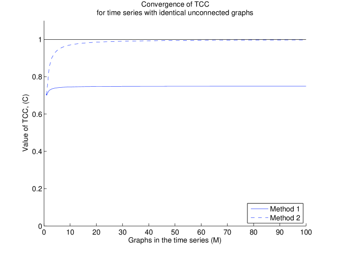
Figure 5: Plot showing convergence behavior of TCC for Methods 1 and 2 for the time series described above, adding identical unconnected graphs to the series in figure (4).

4 Conclusion

Because Method 1 for calculating the temporal correlation coefficient relies on a fixed number of nodes in the network $N$, some modifications (presented as Method 2) need to be made to the formulation to avoid systematically underestimating the correlation between two unconnected graphs. In a time series of graphs which have, on average, unconnected nodes, the temporal correlation coefficient $C$ calculated using Method 1 will underestimate the correlation between two graphs by the fraction $\frac{\bar{N_{0}}}{N}$ where $\bar{N_{0}}$ is the average number of unconnected nodes over time and $N$ is the total number of nodes considered.

References

• [1] V. Nicosia et al. ”Graph Metrics for Temporal Networks”.
arXiv:1306.0493 [physics.soc-ph]