A new method for an objective, $\chi^{2}$-based spectroscopic analysis of early-type stars^,

Abstract

Context. A precise quantitative spectral analysis, encompassing atmospheric parameter and chemical elemental abundance determination, is time-consuming due to its iterative nature and the multi-parameter space to be explored, especially when done by the naked eye.

Aims. A robust automated fitting technique that is as trustworthy as traditional methods would allow for large samples of stars to be analyzed in a consistent manner in reasonable time.

Methods. We present a semi-automated quantitative spectral analysis technique for early-type stars based on the concept of $\chi^{2}$ minimization. The method’s main features are as follows: far less subjectivity than the naked eye, correction for inaccurate continuum normalization, consideration of the whole useful spectral range, and simultaneous sampling of the entire multi-parameter space (effective temperature, surface gravity, microturbulence, macroturbulence, projected rotational velocity, radial velocity, and elemental abundances) to find the global best solution, which is also applicable to composite spectra.

Results. The method is fast, robust, and reliable as seen from formal tests and from a comparison with previous analyses.

Conclusions. Consistent quantitative spectral analyses of large samples of early-type stars can be performed quickly with very high accuracy.

1 Introduction

The chemical evolution of galaxies is dominated by the evolution of early-type stars, since these objects are the progenitors of core-collapse supernovae, and therefore contribute to stellar nucleosynthesis in a pronounced way. In this context, important issues are the effects of rotation, especially for that of rotational mixing, on the evolution of massive stars (e.g., Heger & Langer 2000; Meynet & Maeder 2000), as well as spatial and temporal variations of the chemical composition within the Galactic disk (e.g., Fuhrmann 2008; Przybilla 2008). Quantitative spectroscopic analyses of B- and late O-type stars allow for atmospheric parameters and chemical elemental surface abundances to be inferred with high precision, which directly addresses both of the aforementioned topics (see Nieva & Przybilla 2012). Due to the high frequency of binary systems among early-type stars (see, e.g., Sana et al. 2012; Chini et al. 2012), analysis techniques, which are also able to deal with spectra of double-lined spectroscopic binary systems (SB2) are desirable.

Quantitative spectroscopy is based on the comparison of synthetic and observed spectra. Owing to the multi-dimensionality of the parameter space involved (which include the following for B- and late O-type stars: effective temperature $T_{\mathrm{eff}}$, surface gravity $\log(g\,\mathrm{(cm\,s^{-2})})$, microturbulence $\xi$, macroturbulence $\zeta$, projected rotational velocity $\varv\,\sin(i)$, radial velocity $\varv_{\mathrm{rad}}$, metallicity $Z$, and elemental abundances $\{n(x)\}$), investigations are time-consuming since an iterative approach is required (for details see Nieva & Przybilla 2010). Starting from initial estimates for the entire set of parameters, individual variables are refined by using spectral indicators that are sensitive to as few parameters as possible to reduce the complexity of the problem. In early-type stars of solar metallicity, for instance, Stark-broadened hydrogen and helium lines are primarily affected by changes in $T_{\mathrm{eff}}$, $\log(g)$, and $n(\mathrm{He})$ while they are comparatively insensitive to all others. Consequently, these features allow for the temperature, surface gravity, and helium abundance to be constrained. The use of multiple ionization equilibria, which requires that spectral lines of different ionization stages of the same element indicate equal abundances, yields further constraints on $T_{\mathrm{eff}}$ and $\log(g)$ but also on $\xi$ and $n(x)$. Matching the strength of spectral lines and their shape allows for $\zeta$ and $\varv\,\sin(i)$ to be derived. Because of the highly non-trivial coupling of different parameters, the adjustment of individual variables involves re-evaluation of most of the available indicators, leading to an iterative procedure.

Although those iterative steps can be automated to speed up the investigation (see Lefever et al. 2010), the underlying strategy is still prone to miss the global best solution. On the one hand, not all parameters are varied at the same time but many of them separately so that correlations between them are neglected (see Mokiem et al. 2005). On the other hand, parameters are constrained from selected spectral indicators or windows instead of exploiting the information encoded in the entire spectrum. A global analysis method, which is a method simultaneously probing all parameters while considering the maximum useful spectral range, is therefore our goal.

Automated fitting techniques are suitable for this purpose. Moreover, automation is far less subjective, since the matching of theory and observation is based on a mathematical measure, such as a $\chi^{2}$ criterion instead of visual inspection. This is particularly important when one wants to analyze larger samples in a homogeneous manner. The size of the corresponding multi-parameter space, however, requires calculations of numerous synthetic spectra, which is computationally expensive and, therefore, a major obstacle for automated fitting. To minimize the number of calculations involved, synthetic atmospheres may be computed on demand in the course of the fitting process, as realized by Mokiem et al. (2005). In this way, spectra are computed only if they are actually used. Nevertheless, even very efficient fitting algorithms can take from several dozens to hundreds of iterations to find the best solution, which implies a non-negligible run-time of the fitting process. This drawback can be overcome by making use of pre-calculated model grids in which interpolation between grid points can be used to evaluate the fitting function. Unfortunately, sufficient sampling of the whole multi-parameter space is typically not possible, given its large dimension. Consequently, grid-based fitting methods are usually restricted to small subspaces by either keeping some parameters fixed when computing tailored grids (see Castro et al. 2012) or limiting the allowed parameter range, thus reducing the advantages of global automated fitting.

However, due to some unique properties of spectra of early-type stars, such as the low density of spectral lines and the continuous opacity that is dominated by hydrogen and helium, many parameters – in particular, the elemental abundances of the trace elements – are independent of each other. Exploiting this fact, it is possible to probe the entire parameter space by computing only a tiny fraction of it. Based on this idea, we have developed a grid-based global fitting method that facilitates quick and precise determinations of the atmospheric parameters of B- and late O-type stars, which takes non-local thermodynamic equilibrium (non-LTE) effects into consideration (Sect. 2). Furthermore, it is shown that the accuracy of the analysis is generally not limited by statistics, such as the signal-to-noise ratio (S/N) of the observed spectrum, but rather by systematics, such as the uncertainties in atomic data (Sect. 3). For demonstration purposes, the method is then applied to three well-studied early-type stars in Orion and to three SB2 systems yielding atmospheric and fundamental stellar parameters (Sect. 4). A discussion of the results obtained (Sect. 5) is rounded off by a summary (Sect. 6).

2 Setting up the fitting function

2.1 Input physics: models and codes

Table 1: Model atoms for non-LTE calculations.

Ion	Model atom
H & Przybilla & Butler (2004)
He i/ii	Przybilla (2005)
C ii-iii	Nieva & Przybilla (2006, 2008)
N ii	Przybilla & Butler (2001)
O i/ii	Przybilla et al. (2000), Becker & Butler (1988)
Ne i/ii	Morel & Butler (2008)
Mg ii	Przybilla et al. (2001)
Al ii/iii	Przybilla (in prep.)
Si ii/iii/iv	Przybilla & Butler (in prep.)
S ii/iii	Vrancken et al. (1996), updated
Ar ii	Butler (in prep.)
Fe ii/iii	Becker (1998), Morel et al. (2006)

Synthetic spectra are calculated by following the hybrid, non-LTE approach discussed by Przybilla et al. (2006) and Nieva & Przybilla (2006, 2007, 2008). The structure of the atmosphere, such as the stratification of temperature and density, is based on line-blanketed, plane-parallel, homogeneous, and hydrostatic LTE-model atmospheres calculated with Atlas12 (Kurucz 1996). Deviations from local thermodynamic equilibrium are then accounted for by applying updated versions of Detail and Surface (Giddings 1981; Butler & Giddings 1985). The Detail code numerically solves the coupled radiative transfer and statistical equilibrium equations to obtain population numbers in non-LTE, which in turn are input to the Surface code to compute the final synthetic spectrum that uses more detailed line-broadening data. Comprehensive, state-of-the-art model atoms (see Table 1) allow spectral lines to be modeled with high fidelity for chemical elements accessible in the optical spectra of most B- and late O-type stars. Although partly based on LTE concepts, the hybrid method outlined above is consistent with full non-LTE calculations for B-type stars (see Nieva & Przybilla 2007; Przybilla et al. 2011) but is considerably faster and, most importantly, is able to handle more realistic representations of model atoms. For the first time here, we consistently use the concept of LTE opacity sampling to treat background line opacities (employing the realization of Kurucz 1996) in all computational steps, instead of relying on pre-calculated opacity distribution functions.

2.2 Probing the parameter space

Stellar atmospheres are described by a variety of physical quantities. The implementation of those parameters in synthetic model computations varies depending on their nature. Within the scope of this paper, it is instructive to distinguish between primary atmospheric parameters, which are quantities whose effects can be modeled solely by solving the coupled radiative and structural equations describing an atmosphere, and secondary ones, which are quantities whose effects can be incorporated after an atmosphere has been built. For OB-type stars near the main sequence and their evolved progeny, BA-type supergiants, primary parameters are $T_{\mathrm{eff}}$, $\log(g)$, $\xi$, $Z$, and $\{n(x)\}$, while $\zeta$, $\varv\,\sin(i)$, and $\varv_{\mathrm{rad}}$ are secondary ones. By definition, the effective parameter space for which model atmospheres have to be calculated is therefore spanned by the primary parameters. Given a grid-based fitting method that interpolates a regular multi-dimensional mesh of synthetic spectra, the dimension of this parameter space is the product of the individual dimensions of the primary parameters. Due to this multiplicity, each chemical element included in the analysis drastically increases the number of required models. For instance, calculating a grid with ten elements at nine abundances each implies a factor of $9^{10}$, which has to be multiplied with the dimension given by the remaining primary parameters. Since it is infeasible to compute such a large number of models in a reasonable time, a simplification is necessary. To this end, one can exploit the unique properties of (nearby) early-type stars: Due to their young ages, the metallicity of these stars is very well approximated by the cosmic standard (Nieva & Przybilla 2012), in general, so that $Z=0.014$ can be assumed throughout. In massive stars, the latter implies that all metals can be considered as trace elements, which implies that moderate changes of their abundances do not significantly affect the atmospheric structure. This occurs because their respective bound-free opacities are small compared to hydrogen and helium and because line blanketing is relatively insensitive to abundance changes of a specific metal. Altering the abundance of an individual metal has therefore little to no effect on spectral lines of the other metals, except in the case of line blends. However, the density of lines is low in optical spectra of early-type stars, so that intrinsic blends are actually rare (With some more restrictions, this even applies to the ultraviolet region.). Moreover, many of these line blends are caused by macroscopic flux redistributions, which can be, for example, via macroturbulence, stellar rotation, or the finite resolving power of the spectrograph, and are thus not an issue, since they do not affect the microscopic physics governing radiative transfer. Consequently, instead of calculating $9^{10}$ combinations of abundances, it is sufficient to compute models for nine pre-chosen abundance values for each of the ten species. All of these models contain only lines of one specific trace element, while standard abundances are assumed for the other metals to account for their background opacities. Those $10\times 9$ spectra serve as a basis from which each of the $9^{10}$ combinations can be constructed, such as via multiplication of the normalized base spectra. Note that helium cannot be treated as a trace element, since corresponding abundance changes have serious impacts on the atmospheric structure, for instance, via the mean molecular weight or its contribution to the continuum opacity. Hence, the number of required synthetic models is the product of the dimensions of $T_{\mathrm{eff}}$, $\log(g)$, $\xi$, $n(\mathrm{He})$, and the base dimensions of the trace elements.

2.3 Numerical implementation of the model

From the considerations of the previous subsection, the fitting function is constructed as follows: for each trace element of interest, a multi-dimensional regular mesh spanned by effective temperature ($12\,000$ to $34\,000\,\mathrm{K}$, step size: $1000\,\mathrm{K}$), surface gravity (range depending on temperature but typically within $3.0$ to $4.6\,\mathrm{dex}$, $0.2\,\mathrm{dex}$), microturbulence (range depending on temperature but typically within $0$ to $20\,\mathrm{km\,s^{-1}}$, $2\,\mathrm{km\,s^{-1}}$), helium abundance (solar value minus $0.3\,\mathrm{dex}$ to solar value plus $0.5\,\mathrm{dex}$, $0.2\,\mathrm{dex}$), and abundance of the species itself (typically solar value minus $0.8\,\mathrm{dex}$ to solar value plus $0.8\,\mathrm{dex}$, $0.2\,\mathrm{dex}$) has been calculated in advance. This grid can easily be extended whenever needed. Spectra for arbitrary parameters within the mesh are approximated by linear interpolation. At this point, synthetic models contain only spectral lines of hydrogen, helium, and the element under consideration. To combine the normalized spectra of the individual trace elements, each of them is divided by a model with the same specifications but which contains only hydrogen and helium lines. Multiplying the resulting “corrected spectra” with each other and with the hydrogen-helium model leads to a model that takes all of the primary parameters into account. This simplification is well justified as long as spectral lines of different metals are not blended due to microscopic flux redistributions, such as microturbulence, natural line width, and thermal- or pressure broadening. Furthermore, even for blends of weak spectral lines, the method is a good approximation as interaction effects are tiny in that case. Secondary atmospheric parameters are incorporated afterwards: macroturbulence and stellar rotation via convolution of the synthetic spectrum with a joint profile function, which is obtained from numerical stellar disk integration (Gray 2005) with a linear limb-darkening law (using coefficients by Claret & Bloemen 2011), and radial velocity by shifting the entire wavelength scale, according to the Doppler formula.

2.4 Extension to composite spectra

Multiplicity is an important issue for massive stars, as the majority of them probably resides in systems of two (or more) components (see Sana et al. 2012; Chini et al. 2012). While visual binaries or systems with a much fainter secondary can be treated as single stars in the spectroscopic analysis, this is clearly not the case for double-lined spectroscopic binary systems where features of both stars are visible in the spectrum. Stars classified as chemically peculiar objects based on low-resolution and/or low-S/N spectra might actually be unrecognized SB2 systems where the depths of the absorption lines have been altered due to continuum emission of a companion.

The fitting method presented here is also capable of dealing with composite spectra in a simplified manner. To do so, models for the normalized single-star spectra are created separately for the primary ($f_{\mathrm{p}}$) and secondary ($f_{\mathrm{s}}$) component following the procedure given in Sect. 2.3. To obtain the model for their normalized composite spectrum ($f_{\mathrm{comp}}$), these individual contributions have to be summed up while taking their weights into account. The latter are given by the components’ continuum fluxes ($f_{\mathrm{p,cont}}$, $f_{\mathrm{s,cont}}$) and by the ratio of their projected, effective surface areas, which is parametrized by one additional free parameter $A_{\mathrm{eff,s}}/A_{\mathrm{eff,p}}$:

$$f_{\mathrm{comp}}=\frac{f_{\mathrm{cont,p}}\,f_{\mathrm{p}}+A_{\mathrm{eff,s}}/A_{\mathrm{eff,p}}\,f_{\mathrm{cont,s}}\,f_{\mathrm{s}}}{f_{\mathrm{cont,p}}+A_{\mathrm{eff,s}}/A_{\mathrm{eff,p}}\,f_{\mathrm{cont,s}}}\,.\;$$ (1)

Note that this approach conflates all binary interactions, such as mutual distortions and their respective effects on the emitted spectra into the parameter $A_{\mathrm{eff,s}}/A_{\mathrm{eff,p}}$. Consequently, the geometric interpretation of $A_{\mathrm{eff,s}}/A_{\mathrm{eff,p}}$ as the ratio of the effective surface areas of secondary to primary component is only valid as long as those interactions are negligible, such as for well detached systems. Otherwise, $A_{\mathrm{eff,s}}/A_{\mathrm{eff,p}}$ is a combination of the ratio of effective surface areas and a fudge factor that accounts for all missing interaction effects. Of course, the ability of $A_{\mathrm{eff,s}}/A_{\mathrm{eff,p}}$ to compensate these shortcomings is limited and certainly fails for very close or contact systems where a much more sophisticated method is necessary (see, for instance, Palate & Rauw 2012; Palate et al. 2013). Nevertheless, the approach outlined here offers a very fast and efficient way to derive atmospheric parameters and elemental abundances of SB2 systems from the analysis of a single epoch composite spectrum.

2.5 Comparison with observation

To compare models with observations, the synthetic spectra are finally convolved with the instrumental profile, which is a Gaussian curve whose full width at half maximum $\Delta\lambda=\lambda/R$ is a function of the spectral resolving power $R$.

The goodness of fit of a model is then derived from its absolute $\chi^{2}$:

$$\chi^{2}=\sum\limits_{i}\chi_{i}^{2}=\sum\limits_{i}\left(\frac{f_{i}-f_{{\mathrm{model,}}i}}{\delta_{i}}\right)^{2}\,.\;$$ (2)

Here, $f_{i}$, $f_{{\mathrm{model,}}i}$ and $\delta_{i}$ are the observed flux, model flux and uncertainty in the observed flux at data point $i$, respectively. The sum is taken over all pixels $i$ in the spectrum, which either excludes only those lines that have well-known shortcomings, are missing in our models, or are of non-photospheric origin, such as telluric lines and diffuse interstellar bands. The lower the value of $\chi^{2}$, the better the quality of the fit. Other ways of measuring the fitness exist but may have different properties. One reason to choose a standard $i$-based over a line-based $\chi^{2}$ criterion (as, for instance, done by Simón-Díaz et al. 2011b; Castro et al. 2012) is that it gives lines with more data points a larger weight than those with less information. Moreover, the corresponding $\chi^{2}$ distribution is well studied, which allows statistical uncertainties of the input parameters to be deduced from the $\chi^{2}$ statistics (see Sect. 3.3).

The analysis is carried out completely within the Interactive Spectral Interpretation System (ISIS, Houck & Denicola 2000), which simplifies the investigation tremendously. Apart from many useful functions and tools, various minimization algorithms, such as the simplex or gradient methods are available. As shown in the next section, the $\chi^{2}$ landscape of our problem is generally very well behaved so that the absolute minimum is found after a relatively small number of steps, which allows for quick and efficient analyses.

3 Formal tests and discussion of uncertainties

3.1 Noise estimation

Calculating $\chi^{2}$ requires proper knowledge of the measurement uncertainties $\delta_{i}$, which either are systematic in nature and, for instance, caused by an incorrect continuum normalization, or, more importantly, have statistical fluctuations, such as noise $n_{i}$. The latter can be estimated from an observed spectrum, which does not need to be flux calibrated, in an easy, fast, and robust way when assuming that the noise $n_{i}$ of data point $i$ obeys a Gaussian probability distribution $p(n_{i})$ with a mean value of zero and a priori unknown standard deviation $\sigma_{i}$:

$$p(n_{i})=\frac{1}{\sqrt{2\pi}\sigma_{i}}\exp\left(-\frac{n_{i}^{2}}{2\sigma_{i}^{2}}\right)\,.\;$$ (3)

For small regions (several data points), the measured flux $f_{i}$ as a function of the wavelength $\lambda$ can be approximately written as the sum of a linear function $a+b\lambda_{i}$, which represents the first two terms in a Taylor expansion of the pure signal and a noise component $n_{i}$:

$$f_{i}=a+b\lambda_{i}+n_{i}\,.\;$$ (4)

To estimate the noise level $\sigma_{i}$, consider the quantity $\Delta_{i}$ defined as

$$\Delta_{i} \equiv f_{i}-(w_{i-2}f_{i-2}+w_{i+2}f_{i+2})$$ (5)

$$= n_{i}-w_{i-2}n_{i-2}-w_{i+2}n_{i+2}+a+b\lambda_{i}$$

$$-w_{i-2}(a+b\lambda_{i-2})-w_{i+2}(a+b\lambda_{i+2})\,.\;$$

Here, $w_{i-2}$ and $w_{i+2}$ are weight factors and chosen such that only the noise terms in Eq. (5) remain:

$$\Delta_{i}=n_{i}-w_{i-2}n_{i-2}-w_{i+2}n_{i+2}\,.\;$$ (6)

The reason for comparing $f_{i}$ to the (weighted) average of data points $i-2$ and $i+2$ instead of $i-1$ and $i+1$ is that adjacent pixels are likely correlated. For example, this is due to detector cross-talk or actions taken during data reduction like the wavelength calibration. Assuming that there is no correlation with the next neighbor but one implies that Eq. (3) is valid for points $i$, $i-2$, and $i+2$, and the probability distribution $p(\Delta_{i})$ reads:

$$p(\Delta_{i}) = \int\limits_{-\infty}^{\infty}\int\limits_{-\infty}^{\infty}\int\limits_{-\infty}^{\infty}p(n_{i})p(n_{i-2})p(n_{i+2})$$

$$\delta\left(\Delta_{i}-(n_{i}-w_{i-2}n_{i-2}-w_{i+2}n_{i+2})\right)\mathrm{d}n_{i}\mathrm{d}n_{i-2}\mathrm{d}n_{i+2}\,.\;$$

Here, $\delta$ is the dirac delta function. For adjacent data points, it is well justified to assume $\sigma_{i}=\sigma_{i-2}=\sigma_{i+2}\equiv\sigma$, so that $p(\Delta_{i})$ simplifies to

$$p(\Delta_{i})=\frac{1}{\sqrt{2\pi}\tilde{\sigma}}\exp\left(-\frac{\Delta_{i}^{2}}{2\tilde{\sigma}^{2}}\right),\quad\tilde{\sigma}=\sigma\sqrt{w^{2}_{i-2}+w^{2}_{i+2}+1}\,.\;$$ (8)

Consequently, the distribution of $\Delta_{i}=f_{i}-(w_{i-2}f_{i-2}+w_{i+2}f_{i+2})$ is a Gaussian with a standard deviation $\tilde{\sigma}$ defined by Eq. (8). Extending the assumption of a constant noise level $\sigma_{i}=\sigma$ to a statistically significant number of data points allows $\sigma$, which is the statistical component of the uncertainty $\delta_{i}$ in Eq. (2), to be derived from the measurable distribution of $\Delta_{i}$. If the reduced $\chi^{2}$ at the best fit is larger than $1$, it might also be necessary to consider a systematic component of $\delta_{i}$ (see footnote 7).

3.2 Performance and reliability of the method

Before fitting real spectra, several formal tests were carried out to examine the properties of the automated method. With this aim, mock spectra were constructed from synthetic ones by adding Gaussian-distributed noise that corresponded to different S/N. A spectral range $[3940\,\mathrm{\AA},7000\,\mathrm{\AA}]$ was chosen to match the minimum wavelength coverage of standard high-resolution spectrographs. Regions in that interval that are generally affected by telluric features were excluded. The spectral resolving power was set to $R=45\,000$, which is very close to the resolution of the Echelle spectra which are analyzed in this study.

Table 2 lists the results of this exercise for ten exemplary cases. The input parameters and, thus, the global minimum were recovered with excellent accuracy after only a run-time of few minutes on a standard $3.1$ GHz single-core processor and independent of the choice of the starting parameters within the grid, which shows that our method is fast and reliable.

It is important to stress here that all mock spectra were constructed from complete Surface models, which, in contrast to the fitting function, treat every microscopic line blend correctly by simultaneously computing lines of all chemical species under consideration. Additionally, models off the grid points were chosen to check that our mesh is sufficiently spaced for the linear interpolation scheme applied. Because the differences of input and output values in Table 2 are often covered by the very small statistical uncertainties (see Sect. 3.3) that result from the high S/N assigned to the mock spectra, we conclude that inaccuracies introduced by simplifications in our approach are negligible.

In a second step, three mock composite spectra were created with the help of Eq. (1). The parameters chosen here are motivated by real SB2 systems and anticipate the results presented in Sect. 4. They cover a sharp-lined, well-separated and, thus, easy to analyze system and a very difficult configuration with heavily blended spectral features. Similar to the previous tests, most of the input parameters are recovered with very high precision or at least within the derived uncertainties, as seen in Table 3. In particular, the degree of accuracy in the inferred parameters of both components of the extremely blended composite spectrum is astonishing, hence, making us quite confident that our method is also highly suitable for investigations of SB2 systems.

Although our method is able to model individual abundances if necessary, we generally prefer to assume an identical chemical composition for the two components within the binary system. In this way, the number of free parameters and, consequently, the numerical complexity of the problem is significantly reduced. In cases where the parameters of the secondary component are only poorly constrained due to their little impact on the composite spectrum, it is even necessary to impose these constraints, which compensate for the lack of spectral indicators to derive reasonable atmospheric parameters. Note that the assumption of an equal chemical composition is well justified for SB2 systems containing B-type or late O-type stars. On the one hand, the components of SB2 systems are in general similar regarding to their masses (Otherwise, the flux contribution of the fainter companion would not be visible in the spectrum.), ages (the whole system formed at once), and pristine chemical composition (both components formed from the same building material). On the other hand, processes causing chemical anomalies are rare among B- and late O-type stars and primarily affect helium (Smith 1996). Since chemical peculiarities are possibly even less frequent in detached binary systems (Pavlovski & Southworth 2013), elemental abundances are expected to evolve in the same way in both components. To estimate the influence of this approximation on the spectral analysis, Table 3 lists the results obtained from fitting the three mock composite spectra with adjustable abundances and an equal chemical composition. Even for the system with different individual abundances, the results derived by assuming an identical chemical composition are very satisfying. In particular, this is with respect to the primary component, which dominates the spectrum and in this way also the estimates for the system abundances and their respective confidence limits. As a consequence, the actual abundances of the secondary component may sometimes lie outside of the uncertainty intervals determined for the binary system as a whole. Nevertheless, it is obvious that the decision of whether or not to use separate abundances during the fitting process depends on the individual object and has to be checked, for example, a posteriori by inspecting the final match of the model to the observation.

Table 2: Comparison of input parameters (“In” row) and corresponding parameters obtained from fits (“Out” row) for ten exemplary mock spectra computed from complete Surface models, which simultaneously account for all lines considered in the fitting function.

	S/N	$T_{\mathrm{eff}}$	$\log(g)$	$\varv_{\mathrm{rad}}$	$\varv\,\sin(i)$	$\zeta$	$\xi$		$\log(n(x))$
		(K)	(cgs)	$(\mathrm{km\,s^{-1}})$					He	C	N	O	Ne	Mg	Al	Si	S	Ar	Fe
In	$300$	$15000$	$3.750$	$-18.0$	$15.0$	$7.0$	$2.00$		$-1.06$	$-3.70$	$-4.30$	$-3.20$	$-4.00$	$-4.70$	$-5.60$	$-4.60$	$-4.80$	$-5.60$	$-4.60$
Out	$305$	$15000$	$3.750$	$-18.0$	$14.8$	$8.0$	$2.10$		$-1.06$	$-3.71$	$-4.28$	$-3.20$	$-4.01$	$-4.70$	$-5.60$	$-4.61$	$-4.81$	$-5.68$	$-4.61$
Stat.	${}^{+3}_{-3}$	${}^{+20}_{-20}$	${}^{+0.003}_{-0.004}$	${}^{+0.1}_{-0.1}$	${}^{+0.1}_{-0.1}$	${}^{+0.2}_{-0.1}$	${}^{+0.04}_{-0.03}$		${}^{+0.01}_{-0.01}$	${}^{+0.02}_{-0.02}$	${}^{+0.04}_{-0.04}$	${}^{+0.02}_{-0.02}$	${}^{+0.02}_{-0.02}$	${}^{+0.02}_{-0.02}$	${}^{+0.02}_{-0.02}$	${}^{+0.02}_{-0.02}$	${}^{+0.01}_{-0.01}$	${}^{+0.07}_{-0.08}$	${}^{+0.01}_{-0.01}$
Sys.	…	${}^{+300}_{-300}$	${}^{+0.100}_{-0.100}$	${}^{+0.1}_{-0.1}$	${}^{+0.2}_{-0.1}$	${}^{+0.7}_{-1.2}$	${}^{+0.79}_{-1.09}$		${}^{+0.15}_{-0.09}$	${}^{+0.07}_{-0.09}$	${}^{+0.05}_{-0.08}$	${}^{+0.04}_{-0.08}$	${}^{+0.04}_{-0.02}$	${}^{+0.06}_{-0.07}$	${}^{+0.02}_{-0.02}$	${}^{+0.12}_{-0.18}$	${}^{+0.04}_{-0.04}$	${}^{+0.08}_{-0.14}$	${}^{+0.06}_{-0.10}$
Start	…	$19000$	$3.700$	$-15.0$	$10.0$	$10.0$	$3.00$		$-0.85$	$-3.60$	$-4.20$	$-3.20$	$-4.00$	$-4.60$	$-5.80$	$-4.40$	$-4.90$	$-5.60$	$-4.60$
In	$300$	$15000$	$4.250$	$36.0$	$17.0$	$16.0$	$2.00$		$-1.06$	$-3.70$	$-4.30$	$-3.20$	$-4.00$	$-4.70$	$-5.60$	$-4.60$	$-4.80$	$-5.60$	$-4.60$
Out	$295$	$14860$	$4.215$	$36.0$	$17.0$	$16.1$	$1.90$		$-1.04$	$-3.68$	$-4.32$	$-3.22$	$-4.00$	$-4.72$	$-5.60$	$-4.61$	$-4.80$	$-5.50$	$-4.65$
Stat.	${}^{+2}_{-2}$	${}^{+30}_{-20}$	${}^{+0.008}_{-0.006}$	${}^{+0.1}_{-0.1}$	${}^{+0.1}_{-0.1}$	${}^{+0.3}_{-0.2}$	${}^{+0.07}_{-0.03}$		${}^{+0.01}_{-0.01}$	${}^{+0.02}_{-0.01}$	${}^{+0.07}_{-0.07}$	${}^{+0.01}_{-0.01}$	${}^{+0.02}_{-0.02}$	${}^{+0.02}_{-0.01}$	${}^{+0.02}_{-0.02}$	${}^{+0.02}_{-0.01}$	${}^{+0.01}_{-0.01}$	${}^{+0.10}_{-0.11}$	${}^{+0.01}_{-0.01}$
Sys.	…	${}^{+300}_{-300}$	${}^{+0.100}_{-0.100}$	${}^{+0.1}_{-0.1}$	${}^{+0.1}_{-0.1}$	${}^{+0.2}_{-0.3}$	${}^{+0.62}_{-0.86}$		${}^{+0.15}_{-0.12}$	${}^{+0.07}_{-0.08}$	${}^{+0.06}_{-0.09}$	${}^{+0.07}_{-0.07}$	${}^{+0.06}_{-0.04}$	${}^{+0.06}_{-0.06}$	${}^{+0.02}_{-0.02}$	${}^{+0.11}_{-0.11}$	${}^{+0.04}_{-0.04}$	${}^{+0.08}_{-0.14}$	${}^{+0.08}_{-0.10}$
Start	…	$19000$	$3.700$	$35.0$	$10.0$	$10.0$	$3.00$		$-0.85$	$-3.60$	$-4.20$	$-3.20$	$-4.00$	$-4.60$	$-5.80$	$-4.40$	$-4.90$	$-5.60$	$-4.60$
In	$100$	$20000$	$3.750$	$19.0$	$25.0$	$18.0$	$2.0$		$-1.06$	$-3.70$	$-4.30$	$-3.20$	$-4.00$	$-4.70$	$-5.60$	$-4.60$	$-4.80$	$-5.60$	$-4.60$
Out	$100$	$19960$	$3.734$	$18.9$	$23.5$	$22.0$	$1.94$		$-1.05$	$-3.68$	$-4.28$	$-3.19$	$-4.02$	$-4.71$	$-5.56$	$-4.57$	$-4.78$	$-5.59$	$-4.59$
Stat.	${}^{+1}_{-1}$	${}^{+120}_{-120}$	${}^{+0.015}_{-0.017}$	${}^{+0.3}_{-0.3}$	${}^{+1.1}_{-1.1}$	${}^{+1.7}_{-0.9}$	${}^{+0.3}_{-0.7}$		${}^{+0.02}_{-0.02}$	${}^{+0.04}_{-0.03}$	${}^{+0.04}_{-0.04}$	${}^{+0.04}_{-0.03}$	${}^{+0.04}_{-0.04}$	${}^{+0.06}_{-0.05}$	${}^{+0.05}_{-0.04}$	${}^{+0.07}_{-0.05}$	${}^{+0.03}_{-0.03}$	${}^{+0.06}_{-0.08}$	${}^{+0.05}_{-0.04}$
Sys.	…	${}^{+400}_{-400}$	${}^{+0.100}_{-0.100}$	${}^{+0.1}_{-0.1}$	${}^{+0.2}_{-0.2}$	${}^{+0.7}_{-0.7}$	${}^{+0.8}_{-1.7}$		${}^{+0.09}_{-0.07}$	${}^{+0.08}_{-0.06}$	${}^{+0.08}_{-0.07}$	${}^{+0.11}_{-0.11}$	${}^{+0.04}_{-0.04}$	${}^{+0.11}_{-0.09}$	${}^{+0.08}_{-0.07}$	${}^{+0.14}_{-0.12}$	${}^{+0.05}_{-0.05}$	${}^{+0.05}_{-0.05}$	${}^{+0.05}_{-0.05}$
Start	…	$19000$	$3.700$	$10.0$	$10.0$	$10.0$	$3.0$		$-0.85$	$-3.40$	$-4.10$	$-3.10$	$-4.20$	$-4.80$	$-5.60$	$-4.20$	$-4.70$	$-5.70$	$-4.50$
In	$250$	$20000$	$4.250$	$25.0$	$5.0$	$26.0$	$2.00$		$-1.06$	$-3.70$	$-4.30$	$-3.20$	$-4.00$	$-4.70$	$-5.60$	$-4.60$	$-4.80$	$-5.60$	$-4.60$
Out	$254$	$19990$	$4.251$	$25.0$	$0.0$	$26.9$	$2.26$		$-1.07$	$-3.73$	$-4.31$	$-3.22$	$-4.02$	$-4.72$	$-5.58$	$-4.64$	$-4.81$	$-5.61$	$-4.60$
Stat.	${}^{+2}_{-2}$	${}^{+20}_{-20}$	${}^{+0.003}_{-0.004}$	${}^{+0.1}_{-0.1}$	${}^{+1.8}_{-0.0}$	${}^{+0.1}_{-0.1}$	${}^{+0.12}_{-0.07}$		${}^{+0.01}_{-0.01}$	${}^{+0.02}_{-0.02}$	${}^{+0.02}_{-0.02}$	${}^{+0.02}_{-0.02}$	${}^{+0.02}_{-0.02}$	${}^{+0.02}_{-0.02}$	${}^{+0.02}_{-0.02}$	${}^{+0.02}_{-0.02}$	${}^{+0.01}_{-0.01}$	${}^{+0.03}_{-0.04}$	${}^{+0.02}_{-0.02}$
Sys.	…	${}^{+400}_{-400}$	${}^{+0.100}_{-0.100}$	${}^{+0.1}_{-0.1}$	${}^{+3.4}_{-0.0}$	${}^{+0.1}_{-0.1}$	${}^{+1.04}_{-1.66}$		${}^{+0.08}_{-0.06}$	${}^{+0.09}_{-0.07}$	${}^{+0.07}_{-0.07}$	${}^{+0.11}_{-0.12}$	${}^{+0.04}_{-0.03}$	${}^{+0.12}_{-0.13}$	${}^{+0.06}_{-0.06}$	${}^{+0.13}_{-0.11}$	${}^{+0.06}_{-0.05}$	${}^{+0.05}_{-0.05}$	${}^{+0.01}_{-0.03}$
Start	…	$17000$	$4.000$	$20.0$	$10.0$	$10.0$	$3.00$		$-0.85$	$-3.40$	$-4.10$	$-3.10$	$-3.80$	$-4.40$	$-5.90$	$-4.70$	$-4.80$	$-5.50$	$-4.70$
In	$400$	$25000$	$3.750$	$-25.0$	$40.0$	$28.0$	$2.00$		$-1.06$	$-3.70$	$-4.30$	$-3.20$	$-4.00$	$-4.70$	$-5.60$	$-4.60$	$-4.80$	$-5.60$	$-4.60$
Out	$396$	$24930$	$3.738$	$-25.0$	$39.7$	$28.5$	$2.02$		$-1.07$	$-3.72$	$-4.31$	$-3.21$	$-4.00$	$-4.70$	$-5.61$	$-4.61$	$-4.81$	$-5.63$	$-4.61$
Stat.	${}^{+2}_{-2}$	${}^{+20}_{-20}$	${}^{+0.002}_{-0.003}$	${}^{+0.1}_{-0.1}$	${}^{+0.1}_{-0.1}$	${}^{+0.1}_{-0.3}$	${}^{+0.04}_{-0.04}$		${}^{+0.01}_{-0.01}$	${}^{+0.01}_{-0.01}$	${}^{+0.01}_{-0.02}$	${}^{+0.01}_{-0.01}$	${}^{+0.02}_{-0.02}$	${}^{+0.02}_{-0.02}$	${}^{+0.01}_{-0.01}$	${}^{+0.01}_{-0.01}$	${}^{+0.01}_{-0.01}$	${}^{+0.04}_{-0.04}$	${}^{+0.01}_{-0.01}$
Sys.	…	${}^{+500}_{-500}$	${}^{+0.100}_{-0.100}$	${}^{+0.1}_{-0.1}$	${}^{+0.3}_{-0.1}$	${}^{+1.3}_{-1.5}$	${}^{+0.71}_{-0.02}$		${}^{+0.06}_{-0.07}$	${}^{+0.01}_{-0.06}$	${}^{+0.03}_{-0.03}$	${}^{+0.07}_{-0.08}$	${}^{+0.01}_{-0.02}$	${}^{+0.05}_{-0.08}$	${}^{+0.04}_{-0.06}$	${}^{+0.02}_{-0.06}$	${}^{+0.02}_{-0.03}$	${}^{+0.10}_{-0.12}$	${}^{+0.03}_{-0.03}$
Start	…	$23500$	$3.800$	$-20.0$	$10.0$	$10.0$	$8.00$		$-1.10$	$-3.50$	$-4.10$	$-3.30$	$-4.10$	$-4.50$	$-6.00$	$-4.20$	$-4.70$	$-5.40$	$-4.30$
In	$275$	$25000$	$4.250$	$25.0$	$70.0$	$0.0$	$2.00$		$-1.06$	$-3.70$	$-4.30$	$-3.20$	$-4.00$	$-4.70$	$-5.60$	$-4.60$	$-4.80$	$-5.60$	$-4.60$
Out	$274$	$25010$	$4.259$	$25.0$	$69.8$	$3.6$	$2.00$		$-1.05$	$-3.71$	$-4.29$	$-3.21$	$-3.99$	$-4.68$	$-5.60$	$-4.61$	$-4.82$	$-5.59$	$-4.61$
Stat.	${}^{+1}_{-1}$	${}^{+30}_{-30}$	${}^{+0.003}_{-0.003}$	${}^{+0.2}_{-0.1}$	${}^{+0.1}_{-0.1}$	${}^{+3.7}_{-2.8}$	${}^{+0.06}_{-0.11}$		${}^{+0.01}_{-0.01}$	${}^{+0.02}_{-0.02}$	${}^{+0.01}_{-0.01}$	${}^{+0.01}_{-0.01}$	${}^{+0.03}_{-0.03}$	${}^{+0.03}_{-0.03}$	${}^{+0.02}_{-0.02}$	${}^{+0.02}_{-0.02}$	${}^{+0.02}_{-0.02}$	${}^{+0.05}_{-0.07}$	${}^{+0.02}_{-0.02}$
Sys.	…	${}^{+500}_{-500}$	${}^{+0.100}_{-0.100}$	${}^{+0.1}_{-0.1}$	${}^{+0.5}_{-0.1}$	${}^{+3.5}_{-3.6}$	${}^{+1.41}_{-2.00}$		${}^{+0.06}_{-0.06}$	${}^{+0.08}_{-0.10}$	${}^{+0.03}_{-0.03}$	${}^{+0.12}_{-0.11}$	${}^{+0.02}_{-0.04}$	${}^{+0.09}_{-0.10}$	${}^{+0.04}_{-0.04}$	${}^{+0.12}_{-0.11}$	${}^{+0.07}_{-0.06}$	${}^{+0.12}_{-0.15}$	${}^{+0.05}_{-0.04}$
Start	…	$19000$	$3.700$	$30.0$	$10.0$	$10.0$	$3.00$		$-0.85$	$-3.80$	$-4.40$	$-3.40$	$-4.20$	$-4.80$	$-5.90$	$-4.50$	$-4.70$	$-5.80$	$-4.90$
In	$125$	$30000$	$4.250$	$-15.0$	$0.0$	$18.0$	$2.00$		$-1.06$	$-3.70$	$-4.30$	$-3.20$	$-4.00$	$-4.70$	$-5.60$	$-4.60$	$-4.80$	$-5.60$	$-4.60$
Out	$120$	$30110$	$4.259$	$-15.0$	$5.8$	$16.4$	$1.84$		$-1.04$	$-3.72$	$-4.31$	$-3.21$	$-4.02$	$-4.69$	$-5.61$	$-4.61$	$-4.81$	$-5.47$	$-4.60$
Stat.	${}^{+2}_{-2}$	${}^{+40}_{-60}$	${}^{+0.007}_{-0.013}$	${}^{+0.1}_{-0.1}$	${}^{+0.4}_{-0.5}$	${}^{+0.4}_{-0.4}$	${}^{+0.17}_{-0.14}$		${}^{+0.02}_{-0.02}$	${}^{+0.03}_{-0.02}$	${}^{+0.02}_{-0.02}$	${}^{+0.01}_{-0.02}$	${}^{+0.03}_{-0.03}$	${}^{+0.04}_{-0.04}$	${}^{+0.03}_{-0.03}$	${}^{+0.02}_{-0.02}$	${}^{+0.03}_{-0.03}$	${}^{+0.15}_{-0.24}$	${}^{+0.02}_{-0.02}$
Sys.	…	${}^{+610}_{-610}$	${}^{+0.100}_{-0.100}$	${}^{+0.1}_{-0.1}$	${}^{+1.1}_{-1.2}$	${}^{+0.1}_{-0.1}$	${}^{+0.36}_{-0.32}$		${}^{+0.03}_{-0.03}$	${}^{+0.05}_{-0.06}$	${}^{+0.05}_{-0.05}$	${}^{+0.05}_{-0.03}$	${}^{+0.03}_{-0.02}$	${}^{+0.04}_{-0.04}$	${}^{+0.06}_{-0.06}$	${}^{+0.03}_{-0.03}$	${}^{+0.07}_{-0.06}$	${}^{+0.15}_{-0.17}$	${}^{+0.08}_{-0.08}$
Start	…	$32000$	$4.400$	$-15.0$	$1.0$	$0.0$	$7.00$		$-1.15$	$-3.70$	$-4.10$	$-3.10$	$-4.20$	$-4.70$	$-5.90$	$-4.70$	$-4.60$	$-5.40$	$-4.80$
Mock spectrum as a proxy to the observed spectrum of object #1 in Table 4:
In	$250$	$23880$	$4.127$	$23.0$	$5.0$	$4.0$	$2.00$		$-0.99$	$-3.73$	$-4.30$	$-3.29$	$-4.00$	$-4.57$	$-5.79$	$-4.66$	$-4.88$	$-5.49$	$-4.71$
Out	$232$	$23800$	$4.109$	$23.0$	$4.7$	$4.0$	$2.02$		$-0.99$	$-3.74$	$-4.30$	$-3.30$	$-4.02$	$-4.57$	$-5.80$	$-4.66$	$-4.90$	$-5.51$	$-4.73$
Stat.	${}^{+2}_{-2}$	${}^{+50}_{-50}$	${}^{+0.006}_{-0.007}$	${}^{+0.1}_{-0.1}$	${}^{+0.5}_{-2.9}$	${}^{+2.2}_{-0.4}$	${}^{+0.08}_{-0.11}$		${}^{+0.01}_{-0.01}$	${}^{+0.01}_{-0.01}$	${}^{+0.01}_{-0.01}$	${}^{+0.01}_{-0.01}$	${}^{+0.02}_{-0.02}$	${}^{+0.02}_{-0.02}$	${}^{+0.01}_{-0.01}$	${}^{+0.02}_{-0.02}$	${}^{+0.01}_{-0.02}$	${}^{+0.02}_{-0.02}$	${}^{+0.01}_{-0.01}$
Sys.	…	${}^{+480}_{-480}$	${}^{+0.100}_{-0.100}$	${}^{+0.1}_{-0.1}$	${}^{+0.4}_{-0.6}$	${}^{+1.3}_{-1.5}$	${}^{+0.43}_{-0.90}$		${}^{+0.05}_{-0.05}$	${}^{+0.04}_{-0.03}$	${}^{+0.03}_{-0.02}$	${}^{+0.08}_{-0.08}$	${}^{+0.04}_{-0.04}$	${}^{+0.08}_{-0.07}$	${}^{+0.01}_{-0.02}$	${}^{+0.06}_{-0.05}$	${}^{+0.02}_{-0.03}$	${}^{+0.06}_{-0.06}$	${}^{+0.02}_{-0.02}$
Start	…	$19000$	$3.700$	$20.0$	$10.0$	$10.0$	$3.00$		$-0.90$	$-3.50$	$-4.30$	$-3.30$	$-4.20$	$-4.50$	$-5.80$	$-4.50$	$-4.90$	$-5.50$	$-4.70$
Mock spectrum as a proxy to the observed spectrum of object #2 in Table 4:
In	$250$	$19250$	$4.052$	$31.0$	$7.0$	$17.0$	$2.00$		$-1.00$	$-3.64$	$-4.23$	$-3.21$	$-4.06$	$-4.60$	$-5.71$	$-4.48$	$-4.89$	$-5.57$	$-4.63$
Out	$242$	$19240$	$4.058$	$31.0$	$4.8$	$18.0$	$2.07$		$-1.00$	$-3.64$	$-4.23$	$-3.22$	$-4.06$	$-4.62$	$-5.70$	$-4.51$	$-4.89$	$-5.57$	$-4.65$
Stat.	${}^{+2}_{-2}$	${}^{+20}_{-20}$	${}^{+0.005}_{-0.005}$	${}^{+0.1}_{-0.1}$	${}^{+0.4}_{-0.5}$	${}^{+0.1}_{-0.1}$	${}^{+0.05}_{-0.07}$		${}^{+0.01}_{-0.01}$	${}^{+0.01}_{-0.02}$	${}^{+0.02}_{-0.02}$	${}^{+0.02}_{-0.01}$	${}^{+0.02}_{-0.02}$	${}^{+0.02}_{-0.02}$	${}^{+0.02}_{-0.02}$	${}^{+0.02}_{-0.02}$	${}^{+0.01}_{-0.01}$	${}^{+0.03}_{-0.03}$	${}^{+0.02}_{-0.02}$
Sys.	…	${}^{+390}_{-390}$	${}^{+0.100}_{-0.100}$	${}^{+0.1}_{-0.1}$	${}^{+0.9}_{-3.2}$	${}^{+0.1}_{-0.1}$	${}^{+0.84}_{-1.43}$		${}^{+0.08}_{-0.08}$	${}^{+0.08}_{-0.09}$	${}^{+0.08}_{-0.08}$	${}^{+0.11}_{-0.11}$	${}^{+0.03}_{-0.03}$	${}^{+0.10}_{-0.11}$	${}^{+0.05}_{-0.06}$	${}^{+0.13}_{-0.12}$	${}^{+0.04}_{-0.05}$	${}^{+0.05}_{-0.05}$	${}^{+0.01}_{-0.03}$
Start	…	$17000$	$3.700$	$20.0$	$10.0$	$10.0$	$3.00$		$-0.85$	$-3.50$	$-3.90$	$-3.40$	$-3.80$	$-4.40$	$-5.40$	$-4.00$	$-4.70$	$-5.40$	$-4.80$
Mock spectrum as a proxy to the observed spectrum of object #3 in Table 4:
In	$200$	$29210$	$4.284$	$30.0$	$31.0$	$0.0$	$3.20$		$-1.05$	$-3.71$	$-4.13$	$-3.40$	$-4.01$	$-4.58$	$-5.73$	$-4.66$	$-4.97$	$-5.83$	$-4.62$
Out	$197$	$29190$	$4.273$	$30.1$	$30.8$	$0.0$	$3.12$		$-1.04$	$-3.74$	$-4.13$	$-3.41$	$-4.04$	$-4.63$	$-5.76$	$-4.66$	$-5.00$	$-5.87$	$-4.62$
Stat.	${}^{+1}_{-1}$	${}^{+30}_{-30}$	${}^{+0.005}_{-0.005}$	${}^{+0.1}_{-0.1}$	${}^{+0.1}_{-0.1}$	${}^{+1.8}_{-0.0}$	${}^{+0.08}_{-0.08}$		${}^{+0.01}_{-0.01}$	${}^{+0.02}_{-0.02}$	${}^{+0.01}_{-0.01}$	${}^{+0.01}_{-0.01}$	${}^{+0.03}_{-0.03}$	${}^{+0.03}_{-0.03}$	${}^{+0.03}_{-0.03}$	${}^{+0.02}_{-0.02}$	${}^{+0.03}_{-0.02}$	${}^{+0.21}_{-0.13}$	${}^{+0.02}_{-0.02}$
Sys.	…	${}^{+590}_{-590}$	${}^{+0.100}_{-0.100}$	${}^{+0.1}_{-0.1}$	${}^{+0.1}_{-0.1}$	${}^{+4.6}_{-0.0}$	${}^{+0.50}_{-0.57}$		${}^{+0.04}_{-0.03}$	${}^{+0.03}_{-0.04}$	${}^{+0.05}_{-0.05}$	${}^{+0.04}_{-0.03}$	${}^{+0.04}_{-0.03}$	${}^{+0.05}_{-0.05}$	${}^{+0.06}_{-0.05}$	${}^{+0.04}_{-0.04}$	${}^{+0.06}_{-0.05}$	${}^{+0.32}_{-0.13}$	${}^{+0.09}_{-0.07}$
Start	…	$31000$	$4.300$	$20.0$	$10.0$	$10.0$	$7.00$		$-1.05$	$-3.60$	$-4.20$	$-3.20$	$-4.10$	$-4.60$	$-5.80$	$-4.40$	$-4.90$	$-5.60$	$-4.60$

Table 3: Same as Table 2 but for three exemplary mock composite spectra.

S/N

$T_{\mathrm{eff}}$

$\log(g)$

$\varv_{\mathrm{rad}}$

$\varv\,\sin(i)$

$\zeta$

$\xi$

$A_{\mathrm{eff,s}}/A_{\mathrm{eff,p}}$

$\log(n(x))$

(K)

(cgs)

$(\mathrm{km\,s^{-1}})$

He

C

N

O

Ne

Mg

Al

Si

S

Ar

Fe

Mock spectrum as a proxy to the observed spectrum of object #5 in Table 4 (sharp and well-separated features):

In p

$220$

$16680$

$4.098$

$-84.7$

$7.9$

$11.4$

$2.10$

…

$-0.96$

$-3.55$

$-4.16$

$-3.25$

$-4.04$

$-4.73$

$-5.86$

$-4.45$

$-4.91$

$-5.58$

$-4.66$

Out f

$215$

$16680$

$4.098$

$-84.7$

$6.9$

$12.2$

$2.17$

…

$-0.97$

$-3.56$

$-4.19$

$-3.25$

$-4.03$

$-4.74$

$-5.91$

$-4.47$

$-4.91$

$-5.60$

$-4.68$

Stat.

${}^{+1}_{-1}$

${}^{+80}_{-90}$

${}^{+0.023}_{-0.020}$

${}^{+0.1}_{-0.1}$

${}^{+1.4}_{-1.1}$

${}^{+0.7}_{-1.3}$

${}^{+0.14}_{-0.16}$

…

${}^{+0.02}_{-0.03}$

${}^{+0.03}_{-0.03}$

${}^{+0.04}_{-0.04}$

${}^{+0.02}_{-0.03}$

${}^{+0.02}_{-0.02}$

${}^{+0.03}_{-0.03}$

${}^{+0.04}_{-0.06}$

${}^{+0.03}_{-0.03}$

${}^{+0.02}_{-0.02}$

${}^{+0.07}_{-0.10}$

${}^{+0.02}_{-0.03}$

Sys.

…

${}^{+340}_{-340}$

${}^{+0.100}_{-0.100}$

${}^{+0.1}_{-0.1}$

${}^{+0.7}_{-0.6}$

${}^{+0.8}_{-0.8}$

${}^{+0.27}_{-0.29}$

…

${}^{+0.06}_{-0.07}$

${}^{+0.07}_{-0.07}$

${}^{+0.06}_{-0.07}$

${}^{+0.02}_{-0.02}$

${}^{+0.02}_{-0.02}$

${}^{+0.03}_{-0.03}$

${}^{+0.02}_{-0.03}$

${}^{+0.02}_{-0.03}$

${}^{+0.02}_{-0.03}$

${}^{+0.05}_{-0.06}$

${}^{+0.06}_{-0.06}$

Out i

…

$16660$

$4.096$

$-84.7$

$6.6$

$12.4$

$2.20$

…

$-0.97$

$-3.56$

$-4.18$

$-3.26$

$-4.03$

$-4.75$

$-5.90$

$-4.47$

$-4.91$

$-5.60$

$-4.68$

Stat.

…

${}^{+70}_{-70}$

${}^{+0.017}_{-0.022}$

${}^{+0.1}_{-0.1}$

${}^{+1.4}_{-1.0}$

${}^{+0.9}_{-1.3}$

${}^{+0.13}_{-0.15}$

…

${}^{+0.02}_{-0.02}$

${}^{+0.03}_{-0.03}$

${}^{+0.03}_{-0.04}$

${}^{+0.02}_{-0.02}$

${}^{+0.02}_{-0.02}$

${}^{+0.03}_{-0.03}$

${}^{+0.04}_{-0.05}$

${}^{+0.03}_{-0.03}$

${}^{+0.02}_{-0.02}$

${}^{+0.07}_{-0.11}$

${}^{+0.02}_{-0.03}$

Sys.

…

${}^{+340}_{-340}$

${}^{+0.100}_{-0.100}$

${}^{+0.1}_{-0.1}$

${}^{+0.6}_{-0.5}$

${}^{+0.4}_{-0.8}$

${}^{+0.27}_{-0.26}$

…

${}^{+0.05}_{-0.06}$

${}^{+0.06}_{-0.06}$

${}^{+0.05}_{-0.06}$

${}^{+0.01}_{-0.01}$

${}^{+0.01}_{-0.01}$

${}^{+0.03}_{-0.03}$

${}^{+0.02}_{-0.02}$

${}^{+0.02}_{-0.02}$

${}^{+0.02}_{-0.02}$

${}^{+0.04}_{-0.06}$

${}^{+0.05}_{-0.05}$

Start

…

$15000$

$4.100$

$-80.0$

$10.0$

$10.0$

$3.00$

…

$-0.85$

$-3.60$

$-4.20$

$-3.20$

$-4.00$

$-4.60$

$-5.80$

$-4.40$

$-4.90$

$-5.60$

$-4.60$

In s

…

$13490$

$4.274$

$125.0$

$28.3$

$15.6$

$0.79$

$0.642$

$-0.96$

$-3.55$

$-4.16$

$-3.25$

$-4.04$

$-4.73$

$-5.86$

$-4.45$

$-4.91$

$-5.58$

$-4.66$

Out f

…

$13200$

$4.210$

$125.3$

$29.3$

$14.2$

$0.30$

$0.662$

$-0.91$

$-3.46$

$-4.21$

$-3.29$

$-4.12$

$-4.79$

$-5.73$

$-4.50$

$-4.97$

…

$-4.76$

Stat.

…

${}^{+200}_{-250}$

${}^{+0.050}_{-0.070}$

${}^{+0.5}_{-0.5}$

${}^{+0.8}_{-1.3}$

${}^{+1.7}_{-2.9}$

${}^{+0.33}_{-0.30}$

${}^{+0.020}_{-0.018}$

${}^{+0.10}_{-0.07}$

${}^{+0.13}_{-0.12}$

${}^{+0.26}_{-0.52}$

${}^{+0.06}_{-0.08}$

${}^{+0.13}_{-0.14}$

${}^{+0.06}_{-0.06}$

${}^{+0.13}_{-0.16}$

${}^{+0.05}_{-0.06}$

${}^{+0.11}_{-0.10}$

…

${}^{+0.07}_{-0.09}$

Sys.

…

${}^{+260}_{-360}$

${}^{+0.100}_{-0.100}$

${}^{+0.2}_{-0.2}$

${}^{+0.2}_{-0.6}$

${}^{+0.9}_{-1.2}$

${}^{+0.15}_{-0.22}$

${}^{+0.036}_{-0.033}$

${}^{+0.19}_{-0.17}$

${}^{+0.12}_{-0.12}$

${}^{+0.01}_{-0.06}$

${}^{+0.04}_{-0.07}$

${}^{+0.10}_{-0.11}$

${}^{+0.03}_{-0.04}$

${}^{+0.03}_{-0.04}$

${}^{+0.02}_{-0.02}$

${}^{+0.10}_{-0.09}$

…

${}^{+0.09}_{-0.13}$

Out i

…

$13360$

$4.258$

$125.3$

$28.7$

$15.1$

$0.15$

$0.650$

…

…

…

…

…

…

…

…

…

…

…

Stat.

…

${}^{+80}_{-90}$

${}^{+0.028}_{-0.029}$

${}^{+0.5}_{-0.5}$

${}^{+1.3}_{-1.1}$

${}^{+2.1}_{-2.5}$

${}^{+0.34}_{-0.15}$

${}^{+0.015}_{-0.014}$

…

…

…

…

…

…

…

…

…

…

…

Sys.

…

${}^{+270}_{-270}$

${}^{+0.100}_{-0.113}$

${}^{+0.2}_{-0.3}$

${}^{+0.3}_{-0.3}$

${}^{+1.6}_{-1.3}$

${}^{+0.29}_{-0.15}$

${}^{+0.031}_{-0.032}$

…

…

…

…

…

…

…

…

…

…

…

Start

…

$15000$

$4.100$

$120.0$

$10.0$

$10.0$

$3.00$

$0.800$

$-0.85$

$-3.60$

$-4.20$

$-3.20$

$-4.00$

$-4.60$

$-5.80$

$-4.40$

$-4.90$

$-5.60$

$-4.60$

Mock spectrum as a proxy to the observed spectrum of object #6 in Table 4 (extremely blended features):

In p

$350$

$20600$

$3.485$

$-11.2$

$54.2$

$9.4$

$6.04$

…

$-1.02$

$-3.79$

$-4.38$

$-3.39$

$-4.02$

$-4.74$

$-5.87$

$-4.66$

$-4.99$

$-5.59$

$-4.79$

Out f

$350$

$20740$

$3.502$

$-11.3$

$54.4$

$1.9$

$5.80$

…

$-1.02$

$-3.76$

$-4.37$

$-3.39$

$-4.03$

$-4.74$

$-5.87$

$-4.68$

$-5.02$

$-5.57$

$-4.76$

Stat.

${}^{+2}_{-2}$

${}^{+30}_{-20}$

${}^{+0.005}_{-0.003}$

${}^{+0.2}_{-0.2}$

${}^{+0.2}_{-0.2}$

${}^{+4.4}_{-1.9}$

${}^{+0.07}_{-0.12}$

…

${}^{+0.02}_{-0.03}$

${}^{+0.01}_{-0.01}$

${}^{+0.02}_{-0.01}$

${}^{+0.02}_{-0.02}$

${}^{+0.01}_{-0.03}$

${}^{+0.04}_{-0.02}$

${}^{+0.01}_{-0.02}$

${}^{+0.02}_{-0.01}$

${}^{+0.01}_{-0.04}$

${}^{+0.03}_{-0.04}$

${}^{+0.01}_{-0.01}$

Sys.

…

${}^{+420}_{-420}$

${}^{+0.100}_{-0.100}$

${}^{+0.1}_{-0.1}$

${}^{+0.3}_{-0.1}$

${}^{+3.1}_{-1.9}$

${}^{+0.24}_{-0.49}$

…

${}^{+0.03}_{-0.04}$

${}^{+0.02}_{-0.02}$

${}^{+0.05}_{-0.05}$

${}^{+0.09}_{-0.07}$

${}^{+0.03}_{-0.04}$

${}^{+0.05}_{-0.05}$

${}^{+0.03}_{-0.03}$

${}^{+0.03}_{-0.03}$

${}^{+0.02}_{-0.05}$

${}^{+0.03}_{-0.04}$

${}^{+0.04}_{-0.04}$

Out i

…

$20790$

$3.506$

$-11.3$

$54.4$

$3.1$

$5.74$

…

$-1.01$

$-3.79$

$-4.38$

$-3.41$

$-4.03$

$-4.74$

$-5.87$

$-4.68$

$-5.01$

$-5.59$

$-4.79$

Stat.

…

${}^{+30}_{-30}$

${}^{+0.004}_{-0.004}$

${}^{+0.1}_{-0.1}$

${}^{+0.1}_{-0.1}$

${}^{+0.1}_{-3.1}$

${}^{+0.05}_{-0.02}$

…

${}^{+0.01}_{-0.01}$

${}^{+0.01}_{-0.01}$

${}^{+0.01}_{-0.01}$

${}^{+0.01}_{-0.01}$

${}^{+0.02}_{-0.02}$

${}^{+0.02}_{-0.02}$

${}^{+0.02}_{-0.01}$

${}^{+0.02}_{-0.02}$

${}^{+0.02}_{-0.02}$

${}^{+0.02}_{-0.03}$

${}^{+0.02}_{-0.02}$

Sys.

…

${}^{+420}_{-420}$

${}^{+0.100}_{-0.100}$

${}^{+0.1}_{-0.1}$

${}^{+0.4}_{-0.1}$

${}^{+2.8}_{-3.1}$

${}^{+0.46}_{-0.46}$

…

${}^{+0.01}_{-0.01}$

${}^{+0.01}_{-0.01}$

${}^{+0.02}_{-0.02}$

${}^{+0.04}_{-0.04}$

${}^{+0.01}_{-0.01}$

${}^{+0.02}_{-0.01}$

${}^{+0.02}_{-0.02}$

${}^{+0.02}_{-0.02}$

${}^{+0.01}_{-0.01}$

${}^{+0.02}_{-0.02}$

${}^{+0.02}_{-0.02}$

Start

…

$20000$

$3.500$

$-10.0$

$50.0$

$10.0$

$8.00$

…

$-1.05$

$-3.60$

$-4.20$

$-3.20$

$-4.00$

$-4.60$

$-5.80$

$-4.40$

$-4.90$

$-5.60$

$-4.60$

In s

…

$18610$

$3.227$

$-9.1$

$134.0$

$59.5$

$2.90$

$0.936$

$-1.02$

$-3.79$

$-4.38$

$-3.39$

$-4.02$

$-4.74$

$-5.87$

$-4.66$

$-4.99$

$-5.59$

$-4.79$

Out f

…

$18520$

$3.200$

$-9.6$

$118.0$

$87.0$

$3.82$

$1.085$

$-1.00$

$-3.89$

$-4.40$

$-3.46$

$-4.05$

$-4.75$

$-5.86$

$-4.68$

$-5.01$

$-5.68$

$-4.89$

Stat.

…

${}^{+60}_{-40}$

${}^{+0.003}_{-0.002}$

${}^{+0.4}_{-0.7}$

${}^{+1.6}_{-0.5}$

${}^{+0.5}_{-3.0}$

${}^{+0.16}_{-0.12}$

${}^{+0.008}_{-0.005}$

${}^{+0.02}_{-0.02}$

${}^{+0.04}_{-0.04}$

${}^{+0.03}_{-0.05}$

${}^{+0.04}_{-0.05}$

${}^{+0.04}_{-0.02}$

${}^{+0.05}_{-0.05}$

${}^{+0.03}_{-0.06}$

${}^{+0.03}_{-0.04}$

${}^{+0.03}_{-0.03}$

${}^{+0.06}_{-0.05}$

${}^{+0.04}_{-0.05}$

Sys.

…

${}^{+580}_{-500}$

${}^{+0.124}_{-0.124}$

${}^{+0.3}_{-0.1}$

${}^{+1.3}_{-0.8}$

${}^{+2.0}_{-1.6}$

${}^{+0.52}_{-0.36}$

${}^{+0.069}_{-0.131}$

${}^{+0.06}_{-0.03}$

${}^{+0.07}_{-0.06}$

${}^{+0.09}_{-0.10}$

${}^{+0.11}_{-0.13}$

${}^{+0.06}_{-0.03}$

${}^{+0.10}_{-0.06}$

${}^{+0.06}_{-0.05}$

${}^{+0.04}_{-0.04}$

${}^{+0.07}_{-0.03}$

${}^{+0.04}_{-0.04}$

${}^{+0.06}_{-0.07}$

Out i

…

$18410$

$3.197$

$-9.9$

$120.3$

$84.9$

$3.71$

$1.066$

…

…

…

…

…

…

…

…

…

…

…

Stat.

…

${}^{+70}_{-20}$

${}^{+0.010}_{-0.005}$

${}^{+0.7}_{-0.7}$

${}^{+4.8}_{-0.5}$

${}^{+3.0}_{-3.3}$

${}^{+0.15}_{-0.09}$

${}^{+0.015}_{-0.008}$

…

…

…

…

…

…

…

…

…

…

…

Sys.

…

${}^{+410}_{-390}$

${}^{+0.119}_{-0.111}$

${}^{+0.2}_{-0.2}$

${}^{+0.7}_{-0.6}$

${}^{+1.4}_{-1.5}$

${}^{+0.62}_{-0.71}$

${}^{+0.054}_{-0.061}$

…

…

…

…

…

…

…

…

…

…

…

Start

…

$20000$

$3.500$

$-10.0$

$100.0$

$50.0$

$8.00$

$1.000$

$-1.05$

$-3.60$

$-4.20$

$-3.20$

$-4.00$

$-4.60$

$-5.80$

$-4.40$

$-4.90$

$-5.60$

$-4.60$

Mock spectrum as a proxy to the observed spectrum of object #4 b in Table 4 (but with individual metal abundances for the two components):

In p

$340$

$29710$

$3.669$

$104.0$

$23.7$

$41.2$

$14.92$

…

$-1.17$

$-3.79$

$-4.38$

$-3.39$

$-4.02$

$-4.74$

$-5.87$

$-4.66$

$-4.99$

$-5.59$

$-4.79$

Out f

$353$

$29730$

$3.678$

$103.9$

$24.9$

$39.3$

$15.02$

…

$-1.17$

$-3.81$

$-4.39$

$-3.41$

$-4.03$

$-4.75$

$-5.88$

$-4.68$

$-5.00$

…

$-4.86$

Stat.

${}^{+3}_{-2}$

${}^{+20}_{-40}$

${}^{+0.003}_{-0.003}$

${}^{+0.1}_{-0.1}$

${}^{+0.3}_{-0.3}$

${}^{+0.1}_{-0.1}$

${}^{+0.12}_{-0.09}$

…

${}^{+0.01}_{-0.01}$

${}^{+0.01}_{-0.01}$

${}^{+0.01}_{-0.01}$

${}^{+0.01}_{-0.01}$

${}^{+0.02}_{-0.02}$

${}^{+0.02}_{-0.02}$

${}^{+0.03}_{-0.03}$

${}^{+0.01}_{-0.01}$

${}^{+0.02}_{-0.02}$

…

${}^{+0.05}_{-0.04}$

Sys.

…

${}^{+600}_{-600}$

${}^{+0.100}_{-0.100}$

${}^{+0.1}_{-0.1}$

${}^{+0.9}_{-1.0}$

${}^{+0.3}_{-0.1}$

${}^{+0.48}_{-0.61}$

…

${}^{+0.04}_{-0.04}$

${}^{+0.02}_{-0.01}$

${}^{+0.04}_{-0.04}$

${}^{+0.05}_{-0.05}$

${}^{+0.02}_{-0.02}$

${}^{+0.03}_{-0.03}$

${}^{+0.04}_{-0.03}$

${}^{+0.04}_{-0.04}$

${}^{+0.07}_{-0.06}$

…

${}^{+0.07}_{-0.06}$

Out i

…

$29700$

$3.673$

$103.9$

$24.7$

$39.6$

$14.98$

…

$-1.17$

$-3.81$

$-4.39$

$-3.41$

$-4.04$

$-4.74$

$-5.86$

$-4.68$

$-5.00$

…

$-4.80$

Stat.

…

${}^{+10}_{-20}$

${}^{+0.004}_{-0.003}$

${}^{+0.1}_{-0.1}$

${}^{+0.2}_{-0.1}$

${}^{+0.1}_{-0.1}$

${}^{+0.08}_{-0.05}$

…

${}^{+0.01}_{-0.01}$

${}^{+0.01}_{-0.01}$

${}^{+0.01}_{-0.01}$

${}^{+0.01}_{-0.01}$

${}^{+0.02}_{-0.02}$

${}^{+0.02}_{-0.02}$

${}^{+0.03}_{-0.03}$

${}^{+0.01}_{-0.01}$

${}^{+0.02}_{-0.02}$

…

${}^{+0.04}_{-0.04}$

Sys.

…

${}^{+600}_{-600}$

${}^{+0.100}_{-0.100}$

${}^{+0.1}_{-0.1}$

${}^{+0.8}_{-1.2}$

${}^{+0.3}_{-0.1}$

${}^{+0.50}_{-0.63}$

…

${}^{+0.04}_{-0.03}$

${}^{+0.02}_{-0.02}$

${}^{+0.03}_{-0.04}$

${}^{+0.05}_{-0.05}$

${}^{+0.02}_{-0.02}$

${}^{+0.03}_{-0.03}$

${}^{+0.03}_{-0.03}$

${}^{+0.04}_{-0.04}$

${}^{+0.07}_{-0.06}$

…

${}^{+0.03}_{-0.02}$

Start

…

$31000$

$3.800$

$100.0$

$40.0$

$10.0$

$9.00$

…

$-1.05$

$-3.60$

$-4.20$

$-3.20$

$-4.10$

$-4.60$

$-5.80$

$-4.40$

$-4.90$

$-5.60$

$-4.60$

In s

…

$28070$

$4.343$

$-110.9$

$35.5$

$62.6$

$6.04$

$0.218$

$-1.17$

$-3.76$

$-4.50$

$-3.59$

$-4.07$

$-4.61$

$-5.70$

$-4.71$

$-4.94$

$-5.60$

$-4.69$

Out f

…

$27740$

$4.253$

$-110.2$

$28.2$

$67.7$

$6.50$

$0.221$

$-1.23$

$-3.86$

$-4.50$

$-3.64$

$-4.28$

$-4.45$

$-5.73$

$-4.85$

$-4.96$

…

$-4.64$

Stat.

…

${}^{+120}_{-{\color[rgb]{1,1,1}0}80}$

${}^{+0.019}_{-0.019}$

${}^{+1.0}_{-0.9}$

${}^{+3.0}_{-3.3}$

${}^{+3.0}_{-5.9}$

${}^{+0.70}_{-0.40}$

${}^{+0.001}_{-0.002}$

${}^{+0.05}_{-0.04}$

${}^{+0.08}_{-0.07}$

${}^{+0.05}_{-0.05}$

${}^{+0.03}_{-0.03}$

${}^{+0.20}_{-0.18}$

${}^{+0.31}_{-0.60}$

${}^{+0.09}_{-0.09}$

${}^{+0.06}_{-0.06}$

${}^{+0.08}_{-0.08}$

…

${}^{+0.05}_{-0.05}$

Sys.

…

${}^{+710}_{-880}$

${}^{+0.334}_{-0.523}$

${}^{+1.3}_{-0.6}$

${}^{+4.0}_{-2.5}$

${}^{+0.6}_{-0.2}$

${}^{+1.10}_{-2.00}$

${}^{+0.022}_{-0.012}$

${}^{+0.14}_{-0.11}$

${}^{+0.06}_{-0.05}$

${}^{+0.05}_{-0.07}$

${}^{+0.08}_{-0.03}$

${}^{+0.04}_{-0.03}$

${}^{+0.17}_{-0.26}$

${}^{+0.06}_{-0.05}$

${}^{+0.07}_{-0.03}$

${}^{+0.04}_{-0.03}$

…

${}^{+0.11}_{-0.07}$

Out i

…

$26870$

$4.220$

$-110.7$

$33.5$

$65.0$

$4.74$

$0.231$

…

…

…

…

…

…

…

…

…

…

…

Stat.

…

${}^{+120}_{-140}$

${}^{+0.015}_{-0.018}$

${}^{+0.8}_{-1.0}$

${}^{+2.5}_{-2.7}$

${}^{+2.3}_{-2.9}$

${}^{+0.29}_{-0.30}$

${}^{+0.001}_{-0.002}$

…

…

…

…

…

…

…

…

…

…

…

Sys.

…

${}^{+870}_{-850}$

${}^{+0.366}_{-0.526}$

${}^{+1.3}_{-0.9}$

${}^{+3.8}_{-2.7}$

${}^{+0.6}_{-0.5}$

${}^{+0.74}_{-1.76}$

${}^{+0.016}_{-0.010}$

…

…

…

…

…

…

…

…

…

…

…

Start

…

$23500$

$3.800$

$-100.0$

$30.0$

$10.0$

$8.00$

$0.300$

$-1.05$

$-3.60$

$-4.20$

$-3.20$

$-4.10$

$-4.60$

$-5.80$

$-4.40$

$-4.90$

$-5.60$

$-4.60$

3.3 Discussion of statistical and systematic uncertainties

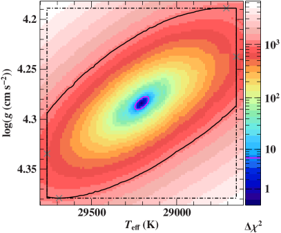
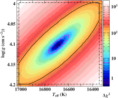
Figure 1: Examples of a color coded $\Delta\chi^{2}$ map as a function of effective temperature and surface gravity for the single star HD 37042 (left) and for the primary component of the SB2 system HD 119109 (right). The magenta line is the $\Delta\chi^{2}=6.63$ contour line, therefore, indicating the statistical (single parameter) 99%-confidence interval for abscissa and ordinate. The four corners of the black dashed-dotted rectangle are defined by the four combinations that result from adding or subtracting the respective total uncertainty, which is a quadratic sum of statistical and systematic uncertainty, to each coordinate of the best fit location. The point of minimum $\Delta\chi^{2}$ on each edge of the rectangle is marked by a gray cross. The solid black line surrounds the region within the rectangle with $\Delta\chi^{2}$ values lower or equal the maximum of the four $\Delta\chi^{2}$ values given by the gray crosses. In this way, areas within the rectangle where the models fit the observation worst are excluded, while it is ensured that each edge of the rectangle contributes at least one point to the solid line at the same time. This construction is our approach to combine statistical and systematic uncertainties.

The accuracy of spectral analyses is generally limited by the quality of the obtained data and the ability of the model to reproduce the observation. As shown in this subsection, shortcomings in the model, which may be due to inaccurate atomic data or deficient line broadening theory, are the main obstacles to overcome to perform more precise investigations.

Statistical uncertainties result from the noise in the observed spectrum and can be deduced from the $\chi^{2}$ statistics in the standard way: starting from the best fit with a reduced $\chi^{2}$ of about one, the parameter under consideration is increased/decreased, while all remaining parameters are fitted, until a certain increment $\Delta\chi^{2}$ from the minimum $\chi^{2}$ is reached (for details, see Bevington & Robinson 1992). Here, each $\Delta\chi^{2}$ corresponds to a confidence level; for example, $\Delta\chi^{2}=6.63$ is equivalent to the 99%-confidence interval (see the magenta line in Fig. 1 for an illustration). The resulting uncertainties are, of course, only trustworthy if the $\delta_{i}$ of Eq. (2) are reasonably estimated. The method outlined in Sect. 3.1 can do so, as shown by the tests with mock spectra with known noise level (see Tables 2 and 3). Moreover, those tests, which use the same models as the fitting routine and, thus, exclude all sources of systematic errors apart from microscopic line blends, give an estimate of the statistical uncertainties that can be expected in real data with a similar S/N.

Systematic uncertainties are much harder to cope with. Sources of systematic errors occur almost everywhere in the course of the analysis (see the discussion in Nieva & Przybilla 2010). At the same time, their effects are by no means trivial, and it is extremely difficult and sometimes even impossible to quantify them. In particular, this is true for atomic data (such as energy levels, oscillator strengths, and photo-ionization cross sections), which affect individual spectral lines and the atmospheric structure. Monte Carlo simulations in the style of Sigut (1996, 1999) offer the possibility of estimating the effects on spectra caused by variations in these input data. However, a thorough error analysis has to take all sources of systematic errors into consideration at the same time to account for correlations as well, which is an unfeasible task.

Our analysis strategy is designed to keep systematic uncertainties as small as possible. For instance, an inaccurate local continuum definition can introduce considerable uncertainties to the determination of metal abundances, especially in fast-rotating stars or low-resolution spectra where metal line blends lower the actual continuum. In our routine, these effects are allowed by re-normalizing the observed spectrum with the help of the synthetic ones. Here, the latter are used to properly locate the continuum regions, which are sufficiently frequent in optical spectra of early-type stars. For these, a correction factor is obtained by dividing the (smoothed) observed data with the model data. Interpolating this factor to the whole wavelength grid gives the local continuum correction term for all spectral lines. For this approach to work, a high degree of completeness in terms of modeled lines is necessary, which is verified by high-resolution, high S/N spectra of slow rotators, as seen in Figs. 2a–2 (available online only).

Another crucial part of our strategy is that we are simultaneously fitting the maximum useful range of the optical spectrum. In this way, parameters are determined not just from one or two spectral indicators but from all available ones. As the systematic errors of the individual indicators are typically independent of each other, which can be exemplified by ionization equilibria of different metals or oscillator strengths of various multiplets, there is a good chance that their effects on the parameter determination average out because some lines systematically give higher and others lower abundances, thus reducing the impact of systematics.

To crudely estimate the systematic uncertainties, we start from the assumption that they mainly appear as inaccuracies in the determination of effective temperature and surface gravity. From our extensive experience with the applied synthetic spectra, we find it realistic but conservative to assign errors of $\pm 2\%$ in $T_{\mathrm{eff}}$ and $\pm 0.1\,\mathrm{dex}$ in $\log(g)$. The ranges given by these errors are formally treated as 99%-confidence intervals. The precision in fixing the microturbulence and the abundances of the chemical elements is then estimated from propagating the errors in $T_{\mathrm{eff}}$ and $\log(g)$. Here, a fit of all remaining parameters is performed for each pixel (that is for each combination of temperature and surface gravity) surrounded by the solid black line in Fig. 1. In the case of a binary system, this procedure is carried out for the secondary component as well. The resulting (combined) ranges of parameter values are then taken to be 99%-confidence intervals. This approach is valid as long as uncertainties induced by variations in $T_{\mathrm{eff}}$ and $\log(g)$ dominate other sources of systematic errors. While this is likely to be true for $\xi$ and $n(x)$, it is clearly not the case for $\varv_{\mathrm{rad}}$, $\varv\,\sin(i)$, and $\zeta$. Determination of radial velocities is generally limited by the accuracy of the wavelength calibration and ranges between $0.1$-$2\,\mathrm{km\,s^{-1}}$ for common spectrographs. Projected rotational velocity and macroturbulence are incorporated via convolution with corresponding profile functions. Because of simplifications (for example in the treatment of limb-darkening or the assumption of radial-tangential macroturbulence) during the derivation of the latter (see Gray 2005), their validity may be limited to a few $\mathrm{km\,s^{-1}}$.

The comparison of statistical and systematic uncertainties, as listed in Table 2, shows that our method’s total uncertainty is dominated by systematic effects down to at least a S/N of $100$. However, this by no means implies that high S/N data are an unnecessary luxury. They are indispensable to detect weak features, such as contributions from a faint companion star, which would otherwise be hidden by noise. Moreover, shortcomings in the models are much more likely to remain unrecognized in low S/N spectra. This is particularly true if they can be partly compensated by tuning some fitting parameters, which, in turn, would cause erroneous results. Instead, this comparison shows that the accuracy of the presented spectral analysis technique is currently limited by modeling and not by observation.

4 Analysis

4.1 The program stars

Table 4: Program stars: ID, spectroscopy, photometry.

#	Star	Instrument	S/N	Photometry	Remark
1	HD 35299	Fies	250	(1), (3), (4), (5)	single
2	HD 35912	Fies	240	(1), (3), (4), (5)	single
3	HD 37042	Fies	205	(2), (3), (4)	single
4 a	HD 75821	Feros	350	(1), (3), (4), (5)	SB2
4 b	HD 75821	Feros	340	(1), (3), (4), (5)	SB2
4 c	HD 75821	Feros	340	(1), (3), (4), (5)	SB2
5	HD 119109	Feros	220	(1), (4), (5)	SB2
6	HD 213420	Fies	350	(1), (3), (4), (5)	SB2

(1) Mermilliod (1991); (2) Ducati (2002); (3) Hauck & Mermilliod (1998); (4) Høg et al. (2000); (5) van Leeuwen (2007).

To illustrate the capabilities of our new method, we re-analyzed three well-studied early-type stars from the Orion region and performed a spectral analysis of three SB2 systems based on very high quality single epoch spectra. For one of the binaries, two additional spectra covering different orbital phases were also investigated. Table 4 lists the relevant information about the program stars. We focused on targets which cover a wide range of effective temperatures, have moderate projected stellar rotations, and show a variety of binary configurations.

4.2 Atmospheric parameters and abundances

Table 5: Atmospheric parameters and abundances of the program stars.

#

$T_{\mathrm{eff}}$

$\log(g)$

$\varv_{\mathrm{rad}}$

$\varv\,\sin(i)$

$\zeta$

$\xi$

$A_{\mathrm{eff,s}}/A_{\mathrm{eff,p}}$

$\log(n(x))$

(K)

(cgs)

$(\mathrm{km\,s^{-1}})$

He

C

N

O

Ne

Mg

Al

Si

S

Ar

Fe

1

$23880$

$4.127$

$23.0$

$5.2$

$4.4$

$2.02$

…

$-0.98$

$-3.73$

$-4.30$

$-3.29$

$-4.00$

$-4.56$

$-5.79$

$-4.66$

$-4.88$

$-5.49$

$-4.71$

Stat.

${}^{+70}_{-70}$

${}^{+0.008}_{-0.008}$

${}^{+0.1}_{-0.1}$

${}^{+0.7}_{-2.2}$

${}^{+2.0}_{-0.7}$

${}^{+0.11}_{-0.23}$

…

${}^{+0.01}_{-0.02}$

${}^{+0.02}_{-0.02}$

${}^{+0.01}_{-0.01}$

${}^{+0.02}_{-0.02}$

${}^{+0.02}_{-0.02}$

${}^{+0.02}_{-0.03}$

${}^{+0.01}_{-0.02}$

${}^{+0.02}_{-0.02}$

${}^{+0.02}_{-0.01}$

${}^{+0.02}_{-0.02}$

${}^{+0.02}_{-0.02}$

Sys.

${}^{+480}_{-480}$

${}^{+0.100}_{-0.100}$

${}^{+0.1}_{-0.1}$

${}^{+0.5}_{-0.3}$

${}^{+0.8}_{-1.5}$

${}^{+0.68}_{-1.39}$

…

${}^{+0.04}_{-0.06}$

${}^{+0.02}_{-0.02}$

${}^{+0.03}_{-0.02}$

${}^{+0.09}_{-0.08}$

${}^{+0.04}_{-0.04}$

${}^{+0.10}_{-0.10}$

${}^{+0.03}_{-0.03}$

${}^{+0.07}_{-0.06}$

${}^{+0.06}_{-0.06}$

${}^{+0.07}_{-0.06}$

${}^{+0.03}_{-0.02}$

1

$24000$

$4.20$

…

$8$

…

$0$

…

$-1.06$

$-3.67$

$-4.23$

$-3.32$

$-3.92$

$-4.43$

…

$-4.54$

…

…

$-4.55$

$\pm 200$

$\pm 0.08$

…

$\pm 1$

…

$\pm 1$

…

…

$\pm 0.07$

$\pm 0.07$

$\pm 0.07$

$\pm 0.09$

$\pm 0.07$

…

$\pm 0.08$

…

…

$\pm 0.10$

2

$19250$

$4.052$

$30.7$

$7.3$

$17.1$

$1.99$

…

$-1.00$

$-3.64$

$-4.23$

$-3.21$

$-4.06$

$-4.60$

$-5.71$

$-4.48$

$-4.89$

$-5.57$

$-4.63$

Stat.

${}^{+60}_{-50}$

${}^{+0.007}_{-0.007}$

${}^{+0.2}_{-0.1}$

${}^{+0.4}_{-0.5}$

${}^{+0.5}_{-1.1}$

${}^{+0.14}_{-0.26}$

…

${}^{+0.01}_{-0.02}$

${}^{+0.03}_{-0.02}$

${}^{+0.02}_{-0.02}$

${}^{+0.02}_{-0.02}$

${}^{+0.02}_{-0.02}$

${}^{+0.02}_{-0.03}$

${}^{+0.03}_{-0.02}$

${}^{+0.03}_{-0.03}$

${}^{+0.02}_{-0.01}$

${}^{+0.03}_{-0.03}$

${}^{+0.02}_{-0.02}$

Sys.

${}^{+390}_{-390}$

${}^{+0.100}_{-0.100}$

${}^{+0.1}_{-0.1}$

${}^{+0.7}_{-1.8}$

${}^{+0.2}_{-0.1}$

${}^{+1.08}_{-1.56}$

…

${}^{+0.08}_{-0.09}$

${}^{+0.07}_{-0.07}$

${}^{+0.08}_{-0.08}$

${}^{+0.10}_{-0.11}$

${}^{+0.03}_{-0.03}$

${}^{+0.11}_{-0.13}$

${}^{+0.06}_{-0.07}$

${}^{+0.13}_{-0.14}$

${}^{+0.05}_{-0.05}$

${}^{+0.04}_{-0.05}$

${}^{+0.01}_{-0.03}$

2

$19000$

$4.00$

…

$15$

$8$

$2$

…

$-1.06$

$-3.71$

$-4.28$

$-3.25$

$-3.99$

$-4.54$

…

$-4.56$

…

…

$-4.52$

$\pm 300$

$\pm 0.10$

…

$\pm 1$

$\pm 1$

$\pm 1$

…

…

$\pm 0.09$

$\pm 0.07$

$\pm 0.09$

$\pm 0.11$

$\pm 0.05$

…

$\pm 0.07$

…

…

$\pm 0.08$

3

$29210$

$4.284$

$29.9$

$30.9$

$0.0$

$3.22$

…

$-1.04$

$-3.71$

$-4.13$

$-3.40$

$-4.01$

$-4.58$

$-5.73$

$-4.66$

$-4.97$

…

$-4.62$

Stat.

${}^{+30}_{-50}$

${}^{+0.006}_{-0.007}$

${}^{+0.2}_{-0.1}$

${}^{+0.1}_{-0.1}$

${}^{+1.1}_{-0.0}$

${}^{+0.10}_{-0.11}$

…

${}^{+0.01}_{-0.02}$

${}^{+0.02}_{-0.02}$

${}^{+0.01}_{-0.01}$

${}^{+0.02}_{-0.01}$

${}^{+0.03}_{-0.03}$

${}^{+0.02}_{-0.03}$

${}^{+0.03}_{-0.02}$

${}^{+0.03}_{-0.01}$

${}^{+0.03}_{-0.03}$

…

${}^{+0.02}_{-0.02}$

Sys.

${}^{+580}_{-590}$

${}^{+0.100}_{-0.100}$

${}^{+0.1}_{-0.1}$

${}^{+0.2}_{-0.1}$

${}^{+2.6}_{-0.0}$

${}^{+0.47}_{-0.59}$

…

${}^{+0.04}_{-0.04}$

${}^{+0.01}_{-0.03}$

${}^{+0.05}_{-0.05}$

${}^{+0.04}_{-0.02}$

${}^{+0.02}_{-0.02}$

${}^{+0.05}_{-0.05}$

${}^{+0.05}_{-0.05}$

${}^{+0.04}_{-0.03}$

${}^{+0.07}_{-0.05}$

…

${}^{+0.08}_{-0.06}$

3

$29300$

$4.30$

…

$30$

$10$

$2$

…

$-1.06$

$-3.71$

$-4.00$

$-3.29$

$-3.91$

$-4.40$

…

$-4.49$

…

…

$-4.50$

$\pm 300$

$\pm 0.09$

…

$\pm 2$

$\pm 3$

$\pm 1$

…

…

$\pm 0.11$

$\pm 0.08$

$\pm 0.08$

$\pm 0.09$

…

…

$\pm 0.03$

…

…

$\pm 0.09$

4p a

$29420$

$3.620$

$17.7$

$24.0$

$37.4$

$13.58$

…

$-1.10$

$-3.81$

$-4.47$

$-3.60$

$-4.10$

$-4.60$

$-5.68$

$-4.70$

$-4.91$

…

$-4.59$

Stat.

${}^{+20}_{-20}$

${}^{+0.003}_{-0.003}$

${}^{+0.2}_{-0.2}$

${}^{+0.7}_{-0.4}$

${}^{+0.2}_{-1.3}$

${}^{+0.12}_{-0.11}$

…

${}^{+0.01}_{-0.01}$

${}^{+0.02}_{-0.01}$

${}^{+0.02}_{-0.01}$

${}^{+0.01}_{-0.01}$

${}^{+0.01}_{-0.02}$

${}^{+0.02}_{-0.01}$

${}^{+0.02}_{-0.01}$

${}^{+0.01}_{-0.01}$

${}^{+0.02}_{-0.03}$

…

${}^{+0.03}_{-0.02}$

Sys.

${}^{+590}_{-590}$

${}^{+0.100}_{-0.100}$

${}^{+1.5}_{-2.0}$

${}^{+2.9}_{-5.0}$

${}^{+0.5}_{-0.1}$

${}^{+0.75}_{-1.04}$

…

${}^{+0.01}_{-0.02}$

${}^{+0.02}_{-0.01}$

${}^{+0.04}_{-0.02}$

${}^{+0.02}_{-0.03}$

${}^{+0.01}_{-0.02}$

${}^{+0.02}_{-0.01}$

${}^{+0.03}_{-0.02}$

${}^{+0.04}_{-0.04}$

${}^{+0.04}_{-0.05}$

…

${}^{+0.05}_{-0.04}$

4s a

$32900$

$4.687$

$56.6$

$0.0$

$69.1$

$14.34$

$0.218$

…

…

…

…

…

…

…

…

…

…

…

Stat.

${}^{+80}_{-80}$

${}^{+0.012}_{-0.014}$

${}^{+0.9}_{-0.6}$

${}^{+7.8}_{-0.0}$

${}^{+1.4}_{-1.1}$

${}^{+0.72}_{-0.53}$

${}^{+0.002}_{-0.007}$

…

…

…

…

…

…

…

…

…

…

…

Sys.

${}^{+{\color[rgb]{1,1,1}0}910}_{-1770}$

${}^{+\geq 0.063}_{-\enspace 0.305}$

${}^{+14.8}_{-18.3}$

${}^{+34.8}_{-{\color[rgb]{1,1,1}0}0.0}$

${}^{+0.8}_{-0.2}$

${}^{+1.66}_{-2.61}$

${}^{+0.314}_{-0.095}$

…

…

…

…

…

…

…

…

…

…

…

4p b

$29710$

$3.669$

$104.0$

$23.7$

$41.2$

$14.92$

…

$-1.17$

$-3.76$

$-4.50$

$-3.59$

$-4.07$

$-4.61$

$-5.70$

$-4.71$

$-4.94$

…

$-4.69$

Stat.

${}^{+40}_{-40}$

${}^{+0.005}_{-0.004}$

${}^{+0.2}_{-0.1}$

${}^{+0.5}_{-0.5}$

${}^{+0.4}_{-0.6}$

${}^{+0.12}_{-0.12}$

…

${}^{+0.01}_{-0.01}$

${}^{+0.02}_{-0.01}$

${}^{+0.02}_{-0.02}$

${}^{+0.01}_{-0.01}$

${}^{+0.02}_{-0.01}$

${}^{+0.02}_{-0.02}$

${}^{+0.02}_{-0.02}$

${}^{+0.01}_{-0.01}$

${}^{+0.02}_{-0.03}$

…

${}^{+0.03}_{-0.03}$

Sys.

${}^{+600}_{-600}$

${}^{+0.100}_{-0.100}$

${}^{+0.1}_{-0.1}$

${}^{+1.2}_{-1.5}$

${}^{+0.1}_{-0.1}$

${}^{+0.27}_{-0.24}$

…

${}^{+0.03}_{-0.03}$

${}^{+0.02}_{-0.01}$

${}^{+0.06}_{-0.05}$

${}^{+0.05}_{-0.05}$

${}^{+0.02}_{-0.01}$

${}^{+0.03}_{-0.03}$

${}^{+0.04}_{-0.04}$

${}^{+0.05}_{-0.05}$

${}^{+0.07}_{-0.07}$

…

${}^{+0.05}_{-0.06}$

4s b

$28070$

$4.343$

$-110.9$

$35.5$

$62.6$

$6.04$

$0.218$

…

…

…

…

…

…

…

…

…

…

…

Stat.

${}^{+140}_{-170}$

${}^{+0.016}_{-0.021}$

${}^{+0.8}_{-1.0}$

${}^{+2.7}_{-2.8}$

${}^{+3.5}_{-3.4}$

${}^{+0.23}_{-0.35}$

${}^{+0.003}_{-0.002}$

…

…

…

…

…

…

…

…

…

…

…

Sys.

${}^{+610}_{-870}$

${}^{+0.310}_{-0.434}$

${}^{+0.6}_{-0.4}$

${}^{+2.6}_{-1.9}$

${}^{+0.4}_{-0.6}$

${}^{+0.78}_{-0.80}$

${}^{+0.014}_{-0.011}$

…

…

…

…

…

…

…

…

…

…

…

4p c

$29630$

$3.622$

$-17.2$

$22.4$

$37.2$

$14.68$

…

$-1.17$

$-3.78$

$-4.57$

$-3.58$

$-4.00$

$-4.60$

$-5.71$

$-4.70$

$-4.92$

…

$-4.65$

Stat.

${}^{+20}_{-20}$

${}^{+0.003}_{-0.003}$

${}^{+0.2}_{-0.1}$

${}^{+0.4}_{-0.5}$

${}^{+0.2}_{-0.1}$

${}^{+0.12}_{-0.12}$

…

${}^{+0.01}_{-0.01}$

${}^{+0.01}_{-0.02}$

${}^{+0.02}_{-0.02}$

${}^{+0.01}_{-0.01}$

${}^{+0.01}_{-0.02}$

${}^{+0.02}_{-0.01}$

${}^{+0.02}_{-0.03}$

${}^{+0.01}_{-0.01}$

${}^{+0.03}_{-0.02}$

…

${}^{+0.03}_{-0.03}$

Sys.

${}^{+600}_{-600}$

${}^{+0.100}_{-0.100}$

${}^{+0.5}_{-1.0}$

${}^{+1.4}_{-8.9}$

${}^{+1.1}_{-0.1}$

${}^{+0.48}_{-0.19}$

…

${}^{+0.03}_{-0.02}$

${}^{+0.01}_{-0.02}$

${}^{+0.03}_{-0.03}$

${}^{+0.05}_{-0.04}$

${}^{+0.02}_{-0.02}$

${}^{+0.03}_{-0.02}$

${}^{+0.03}_{-0.04}$

${}^{+0.05}_{-0.05}$

${}^{+0.06}_{-0.05}$

…

${}^{+0.05}_{-0.04}$

4s c

$30630$

$4.750$

$83.5$

$68.9$

$38.3$

$9.73$

$0.228$

…

…

…

…

…

…

…

…

…

…

…

Stat.

${}^{+140}_{-150}$

${}^{+\ldots}_{-0.013}$

${}^{+1.0}_{-1.0}$

${}^{+0.1}_{-2.8}$

${}^{+4.1}_{-4.2}$

${}^{+0.50}_{-0.47}$

${}^{+0.003}_{-0.003}$

…

…

…

…

…

…

…

…

…

…

…

Sys.

${}^{+{\color[rgb]{1,1,1}0}780}_{-1130}$

${}^{+\ldots}_{-0.358}$

${}^{+{\color[rgb]{1,1,1}0}4.4}_{-36.2}$

${}^{+42.1}_{-{\color[rgb]{1,1,1}0}0.8}$

${}^{+37.7}_{-22.1}$

${}^{+0.97}_{-0.73}$

${}^{+0.204}_{-0.034}$

…

…

…

…

…

…

…

…

…

…

…

5p

$16680$

$4.098$

$-84.7$

$7.9$

$11.4$

$2.10$

…

$-0.96$

$-3.55$

$-4.16$

$-3.25$

$-4.04$

$-4.73$

$-5.86$

$-4.45$

$-4.91$

$-5.58$

$-4.66$

Stat.

${}^{+100}_{-{\color[rgb]{1,1,1}0}90}$

${}^{+0.027}_{-0.021}$

${}^{+0.1}_{-0.2}$

${}^{+1.9}_{-1.3}$

${}^{+1.0}_{-2.2}$

${}^{+0.17}_{-0.19}$

…

${}^{+0.02}_{-0.02}$

${}^{+0.03}_{-0.03}$

${}^{+0.03}_{-0.04}$

${}^{+0.02}_{-0.03}$

${}^{+0.02}_{-0.03}$

${}^{+0.04}_{-0.03}$

${}^{+0.05}_{-0.04}$

${}^{+0.03}_{-0.03}$

${}^{+0.02}_{-0.03}$

${}^{+0.06}_{-0.08}$

${}^{+0.03}_{-0.03}$

Sys.

${}^{+330}_{-340}$

${}^{+0.100}_{-0.100}$

${}^{+0.1}_{-0.1}$

${}^{+1.2}_{-0.2}$

${}^{+0.5}_{-1.7}$

${}^{+0.25}_{-0.29}$

…

${}^{+0.06}_{-0.06}$

${}^{+0.06}_{-0.06}$

${}^{+0.06}_{-0.06}$

${}^{+0.01}_{-0.02}$

${}^{+0.01}_{-0.02}$

${}^{+0.04}_{-0.03}$

${}^{+0.03}_{-0.03}$

${}^{+0.01}_{-0.03}$

${}^{+0.02}_{-0.03}$

${}^{+0.04}_{-0.05}$

${}^{+0.04}_{-0.05}$

5s

$13490$

$4.274$

$125.0$

$28.3$

$15.6$

$0.79$

$0.642$

…

…

…

…

…

…

…

…

…

…

…

Stat.

${}^{+90}_{-80}$

${}^{+0.030}_{-0.025}$

${}^{+0.5}_{-0.4}$

${}^{+1.1}_{-1.5}$

${}^{+3.1}_{-2.0}$

${}^{+0.32}_{-0.31}$

${}^{+0.015}_{-0.013}$

…

…

…

…

…

…

…

…

…

…

…

Sys.

${}^{+270}_{-280}$

${}^{+0.100}_{-0.102}$

${}^{+0.1}_{-0.2}$

${}^{+0.2}_{-0.3}$

${}^{+1.6}_{-0.7}$

${}^{+0.23}_{-0.23}$

${}^{+0.027}_{-0.028}$

…

…

…

…

…

…

…

…

…

…

…

6p

$20590$

$3.485$

$-11.2$

$54.2$

$9.4$

$6.04$

…

$-1.02$

$-3.79$

$-4.38$

$-3.39$

$-4.02$

$-4.74$

$-5.87$

$-4.66$

$-4.98$

$-5.59$

$-4.78$

Stat.

${}^{+30}_{-40}$

${}^{+0.004}_{-0.005}$

${}^{+0.3}_{-0.2}$

${}^{+0.1}_{-0.1}$

${}^{+0.1}_{-2.2}$

${}^{+0.09}_{-0.08}$

…

${}^{+0.01}_{-0.02}$

${}^{+0.02}_{-0.02}$

${}^{+0.01}_{-0.02}$

${}^{+0.02}_{-0.01}$

${}^{+0.02}_{-0.02}$

${}^{+0.02}_{-0.03}$

${}^{+0.02}_{-0.02}$

${}^{+0.02}_{-0.02}$

${}^{+0.01}_{-0.02}$

${}^{+0.02}_{-0.03}$

${}^{+0.02}_{-0.02}$

Sys.

${}^{+420}_{-410}$

${}^{+0.100}_{-0.100}$

${}^{+0.1}_{-0.1}$

${}^{+0.3}_{-0.1}$

${}^{+1.7}_{-3.2}$

${}^{+0.60}_{-0.61}$

…

${}^{+0.01}_{-0.02}$

${}^{+0.02}_{-0.01}$

${}^{+0.02}_{-0.03}$

${}^{+0.06}_{-0.04}$

${}^{+0.02}_{-0.01}$

${}^{+0.02}_{-0.02}$

${}^{+0.02}_{-0.03}$

${}^{+0.03}_{-0.03}$

${}^{+0.01}_{-0.03}$

${}^{+0.01}_{-0.03}$

${}^{+0.02}_{-0.02}$

6s

$18610$

$3.227$

$-9.1$

$134.0$

$59.5$

$2.90$

$0.936$

…

…

…

…

…

…

…

…

…

…

…

Stat.

${}^{+50}_{-70}$

${}^{+0.004}_{-0.006}$

${}^{+1.1}_{-1.0}$

${}^{+0.1}_{-0.6}$

${}^{+4.3}_{-4.7}$

${}^{+0.18}_{-0.18}$

${}^{+0.014}_{-0.015}$

…

…

…

…

…

…

…

…

…

…

…

Sys.

${}^{+460}_{-370}$

${}^{+0.148}_{-0.130}$

${}^{+0.3}_{-0.2}$

${}^{+0.5}_{-0.8}$

${}^{+2.2}_{-1.8}$

${}^{+0.96}_{-0.82}$

${}^{+0.069}_{-0.060}$

…

…

…

…

…

…

…

…

…

…

…

☉

$-1.06$

$-3.57$

$-4.17$

$-3.31$

$-4.07$

$-4.40$

$-5.55$

$-4.49$

$-4.88$

$-5.60$

$-4.50$

${}^{+0.01}_{-0.01}$

${}^{+0.05}_{-0.05}$

${}^{+0.05}_{-0.05}$

${}^{+0.05}_{-0.05}$

${}^{+0.10}_{-0.10}$

${}^{+0.04}_{-0.04}$

${}^{+0.03}_{-0.03}$

${}^{+0.04}_{-0.04}$

${}^{+0.03}_{-0.03}$

${}^{+0.13}_{-0.13}$

${}^{+0.04}_{-0.04}$

Atmospheric parameters and abundances are determined by fitting synthetic to observed spectra, as outlined in detail in Sect. 2. Comparisons of final, best-fitting models with observations are shown for a large portion of the used spectral range in Figs. 2a–2 for the Orion stars and in Figs. 3a–3 (available online only) for the SB2 systems. The overall match of metal lines is almost perfect for the cooler stars of the sample and still very good for the hotter ones where our model atoms begin to be partially incomplete because they were not optimized for this temperature regime. This is particularly true with respect to O ii lines. Consequently, more regions have to be excluded from the analysis for higher effective temperatures due to (blends with) missing spectral lines.

Note that we generally exclude several He i lines from the analysis owing to recurrent issues with their detailed spectral line shapes, which is apparent only in high-resolution spectra with high S/N. This specifically affects the diffuse He I lines that show small but perceptible systematic deficiencies in their forbidden components, which can be attributed to shortcomings in their line broadening theory. These issues are independent of $T_{\mathrm{eff}}$ and $\log(g)$ and cannot be resolved, even if these lines are fitted individually. With a sufficient number of alternative, highly trustworthy He I lines present in the optical spectral range, we generally refrain from fitting the diffuse lines to avoid a possible source of systematic error and use them instead as a consistency check. Nevertheless, given the fact that the synthetic profiles of these lines match the observed ones quite well, except for the forbidden components (see Figs. 2a–2), this decision is probably too restrictive. The diffuse He I lines could therefore be considered for spectral fitting as well with resulting changes in parameters that are well below the stated systematic uncertainties.

Furthermore, we ignore the temperature-sensitive cores of the Balmer lines during the fitting process by excluding those parts of these lines where their normalized flux is smaller than a cutoff, which is typically chosen to be $0.8$. The reason for this is that they are formed in the outer stellar atmosphere, where deviations from the LTE stratification are more pronounced (see Nieva & Przybilla 2007; Przybilla et al. 2011) and where the assumption of hydrostatic equilibrium also becomes less and less valid in the accelerating (weak) stellar wind. Moreover, by simultaneously fitting the entire useful spectral range, there are enough other indicators for $T_{\mathrm{eff}}$ such as (multiple) ionization equilibria available so that it is sufficient to use the Balmer line cores as a consistency check (Figures 2a–2 and Figs. 3a–3 show how well this works.). As a side product, we also reduce the otherwise overwhelming influence of these lines on the parameter determination.

Table 5 lists the atmospheric parameters and abundances of the program stars. Instead of the “classical” notation for the abundance, $\log(x/\mathrm{H})+12$, we have chosen $n(x)$, which is the fractional particle number of species $x$ with respect to all elements. The motivation for this is that the helium abundance is variable from star to star, which, in turn, causes the hydrogen abundance to vary since hydrogen and helium abundances are coupled via the fixed number of total particles. As a consequence, the quantity $\log(x/\mathrm{H})$ can change even if $x$ stays constant. For a better comparison of metal abundances in stars with different helium content, we therefore prefer the notation that gives abundances relative to all elements.

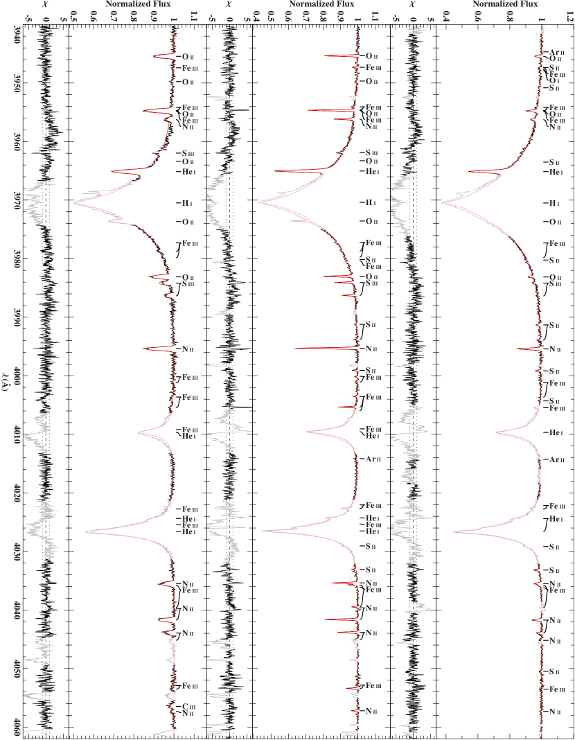
Figure 2a: Comparison of best-fitting model spectrum (red line) with re-normalized observation (black line) for the stars, HD 35912 (right), HD 35299 (middle), and HD 37042 (left), in the spectral range $\lambda\lambda$ 3940–4062 Å. Light colors mark regions that have been excluded from fitting due to the presence of features that are not (properly) included in our models. For the sake of clarity, only the strongest out of all lines that have been used in the analysis are labeled. The residuals $\chi$ are defined by the bracket in Eq. (2).

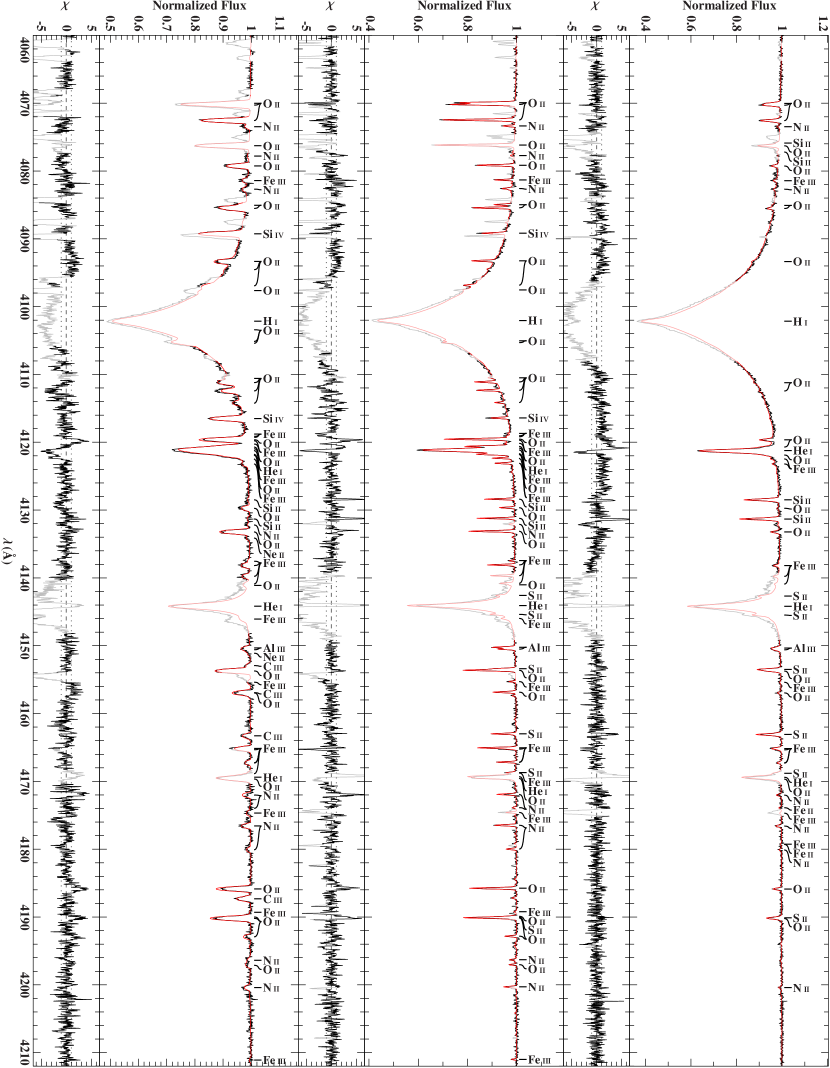
Figure 2: Same as Fig. 2a in the spectral range $\lambda\lambda$ 4060–4212 Å.

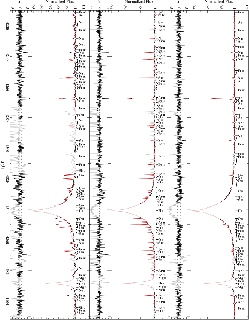
Figure 2: Same as Fig. 2a in the spectral range $\lambda\lambda$ 4210–4412 Å.

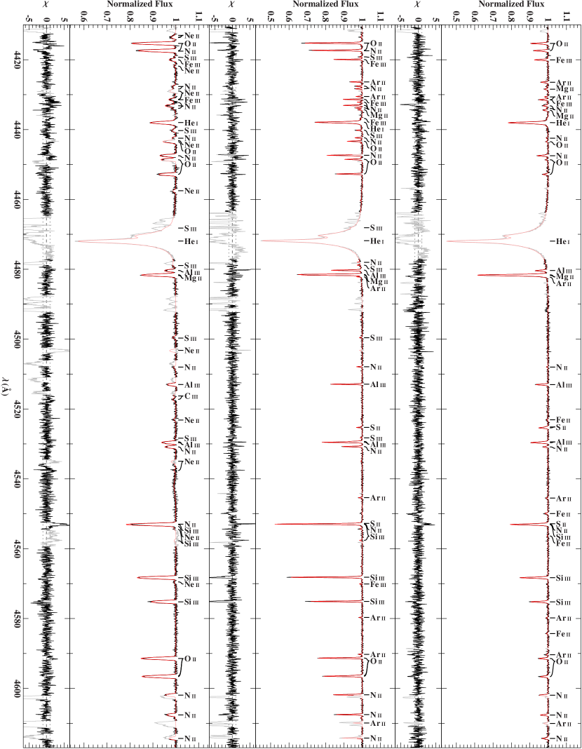
Figure 2: Same as Fig. 2a in the spectral range $\lambda\lambda$ 4410–4617 Å.

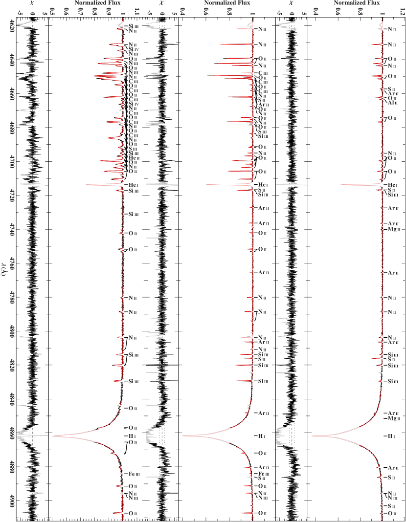
Figure 2: Same as Fig. 2a in the spectral range $\lambda\lambda$ 4615–4912 Å.

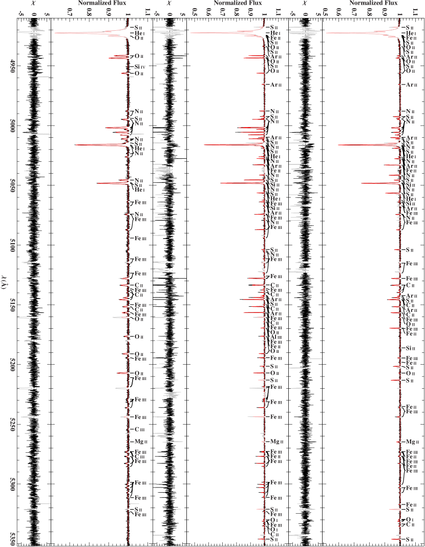
Figure 2: Same as Fig. 2a in the spectral range $\lambda\lambda$ 4910–5352 Å.

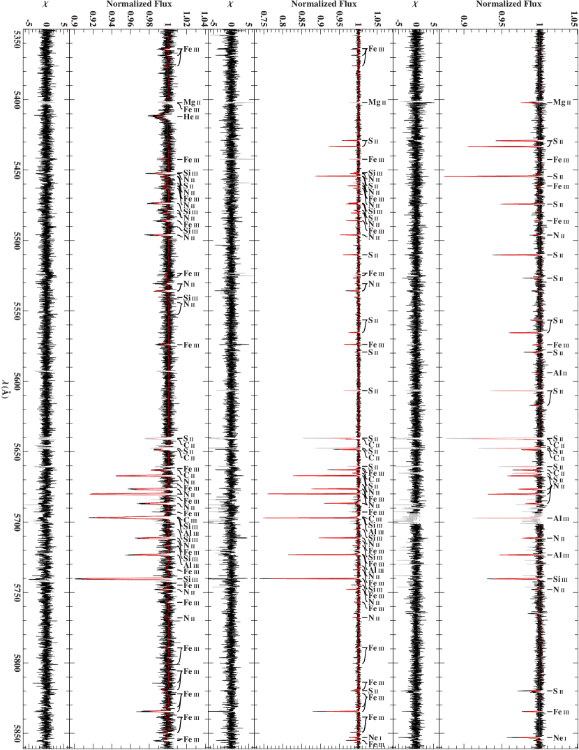
Figure 2: Same as Fig. 2a in the spectral range $\lambda\lambda$ 5350–5861 Å. Note the comparatively small ordinate scales.

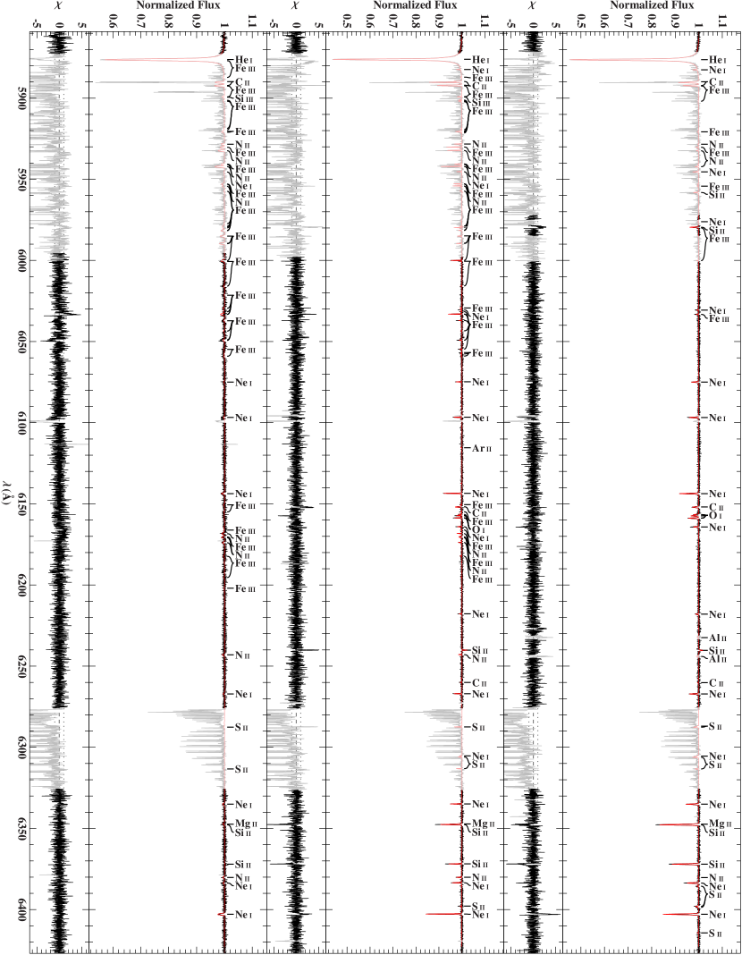
Figure 2: Same as Fig. 2a in the spectral range $\lambda\lambda$ 5859–6427 Å. Strong contamination with telluric lines.

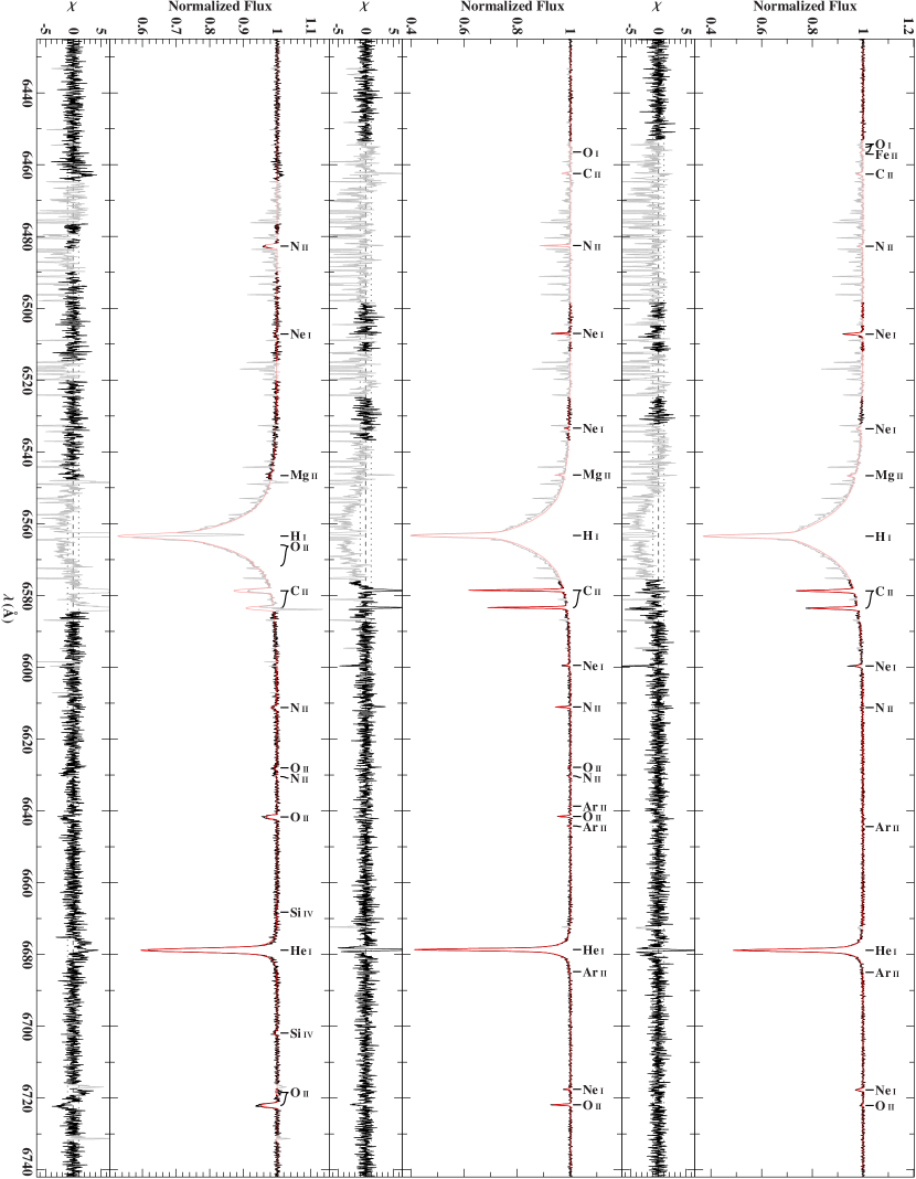
Figure 2: Same as Fig. 2a in the spectral range $\lambda\lambda$ 6425–6742 Å. Strong contamination with telluric lines. Nebula emission lines visible in HD 37042’s spectrum (left).

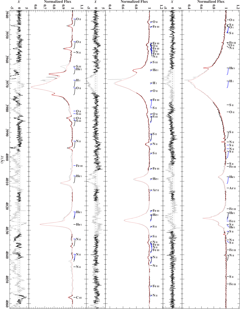
Figure 3a: Comparison of best-fitting model spectrum (red line) with re-normalized observation (black line) for the objects, HD 119109 (right), HD 213420 (middle), and HD 75821 (left), in the spectral range $\lambda\lambda$ 3940–4062 Å. Light colors mark regions that have been excluded from the fitting due to the presence of features that are not (properly) included in our models. For the sake of clarity, only the strongest out of all lines that have been used in the analysis are labeled. Blue connection lines mark contributions of the secondary component. The residuals $\chi$ are defined by the bracket in Eq. (2).

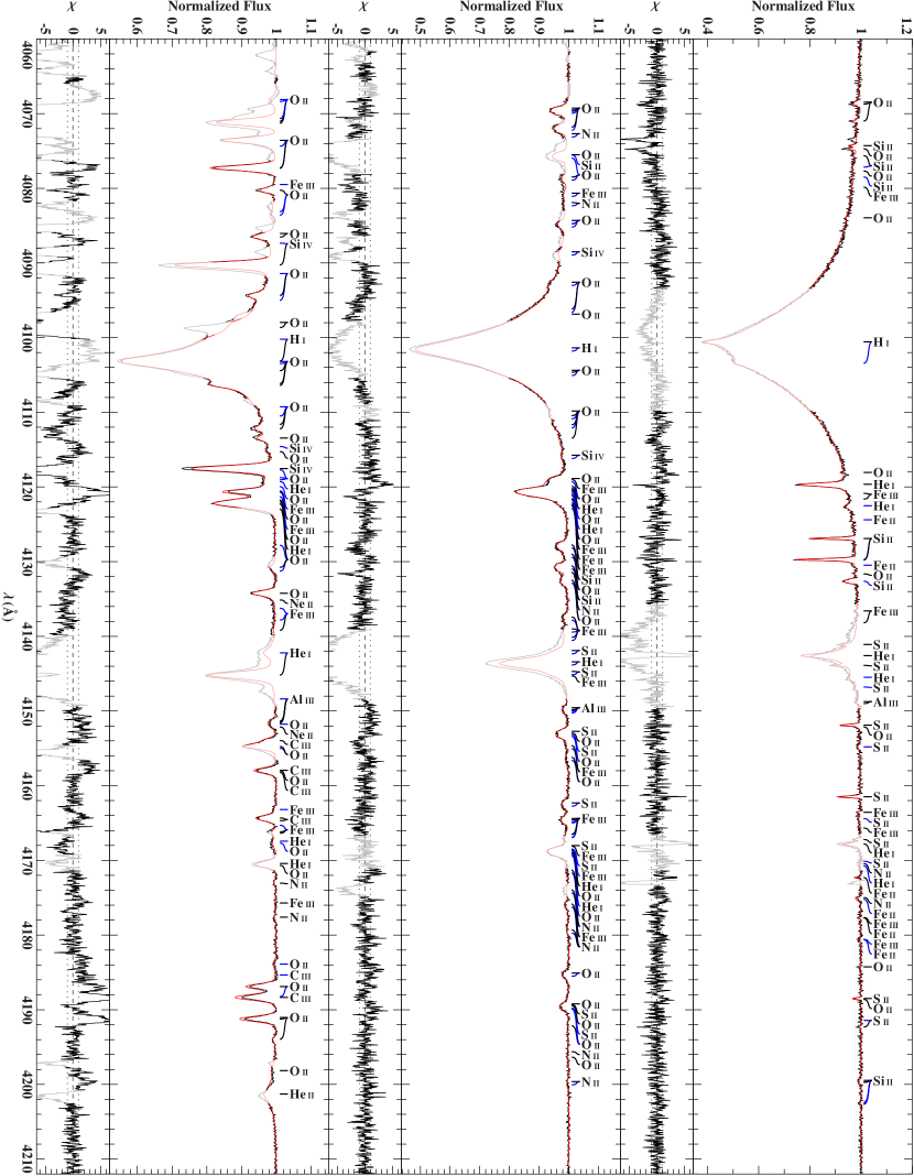
Figure 3: Same as Fig. 3a in the spectral range $\lambda\lambda$ 4060–4212 Å.

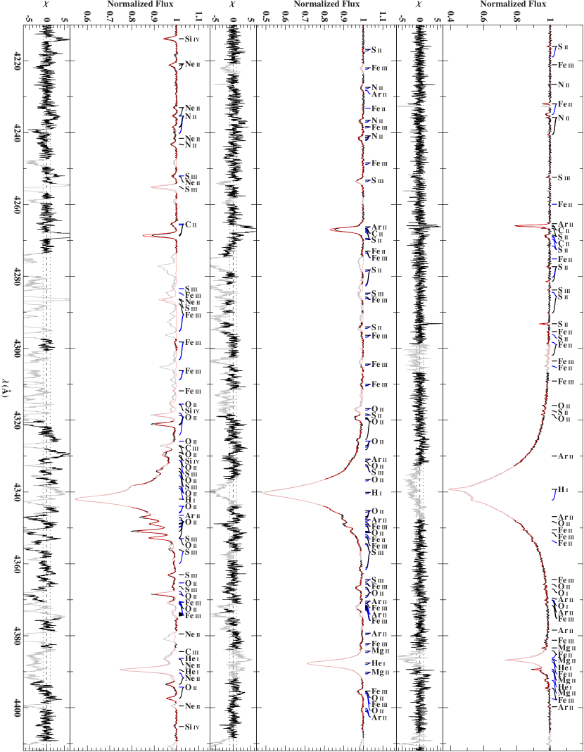
Figure 3: Same as Fig. 3a in the spectral range $\lambda\lambda$ 4210–4412 Å.

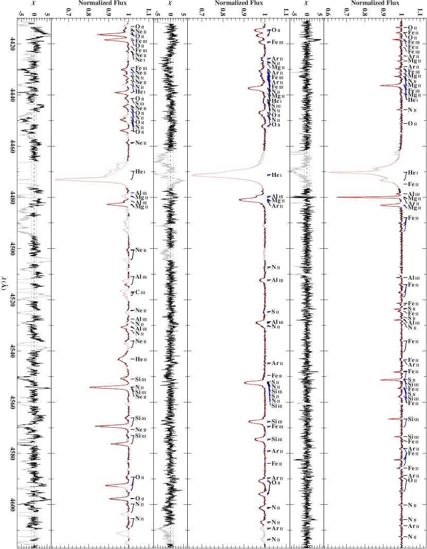
Figure 3: Same as Fig. 3a in the spectral range $\lambda\lambda$ 4410–4617 Å.

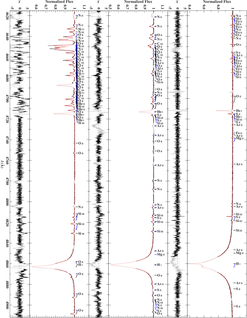
Figure 3: Same as Fig. 3a in the spectral range $\lambda\lambda$ 4615–4912 Å.

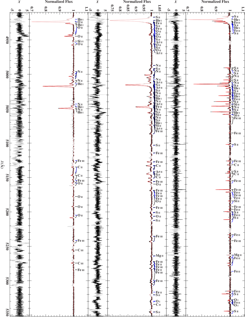
Figure 3: Same as Fig. 3a in the spectral range $\lambda\lambda$ 4910–5352 Å.

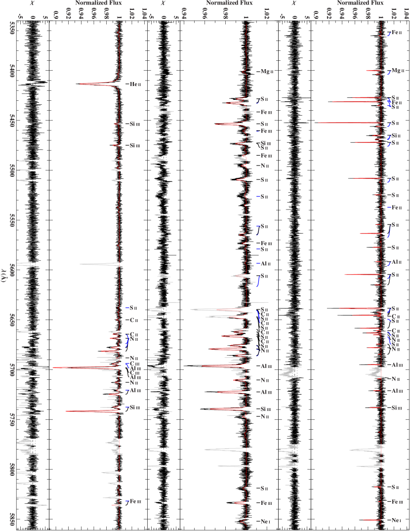
Figure 3: Same as Fig. 3a in the spectral range $\lambda\lambda$ 5350–5861 Å. Note the comparatively small ordinate scales.

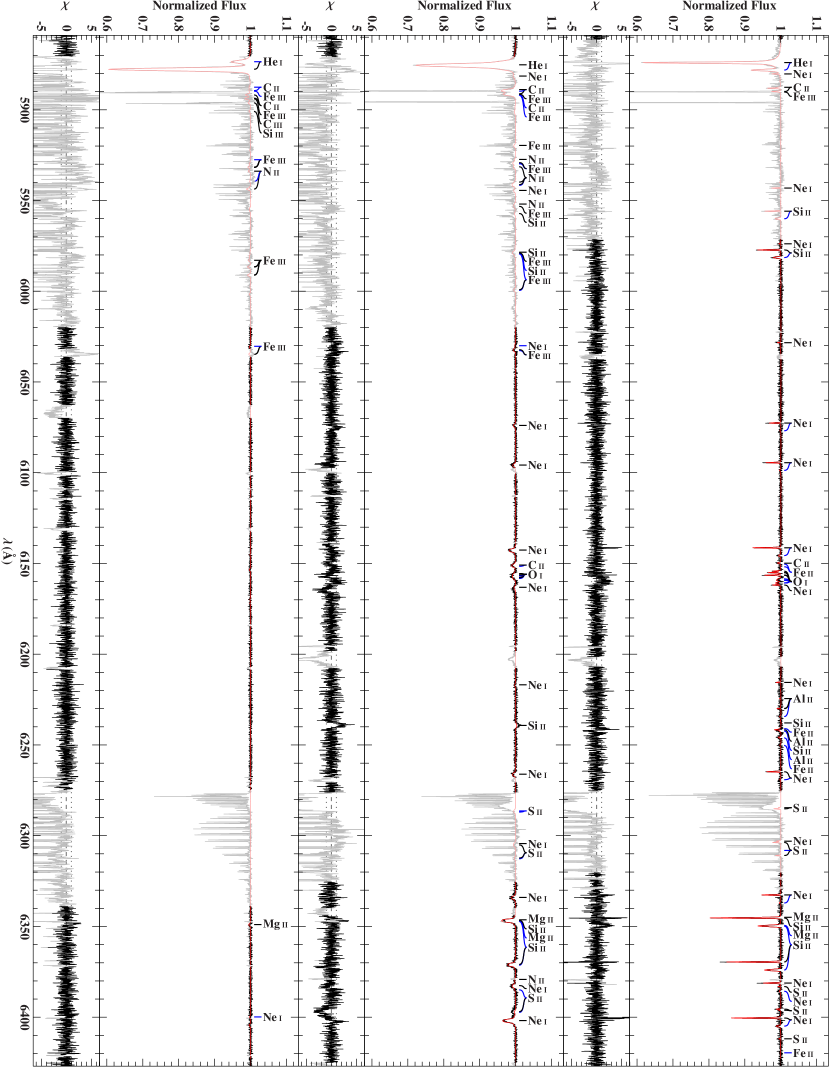
Figure 3: Same as Fig. 3a in the spectral range $\lambda\lambda$ 5859–6427 Å. Strong contamination with telluric lines.

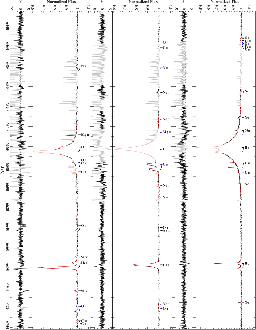
Figure 3: Same as Fig. 3a in the spectral range $\lambda\lambda$ 6425–6742 Å. Strong contamination with telluric lines.

4.3 Stellar parameters and mass fractions

Table 6: Stellar parameters and mass fractions of the program stars.

#		$M$			$\tau$			$\log(L/L_{\sun})$			$R_{\star}$			$d$			$\Pi^{-1}$			$X$			$Y$			$Z$
		$(M_{\sun})$			(Myr)						$(R_{\sun})$			(pc)
1		$9.3$	${}^{+0.5}_{-0.4}$		$12$	${}^{+4}_{-7}$		$3.75$	${}^{+0.08}_{-0.08}$		$4.4$	${}^{+0.6}_{-0.6}$		$380$	${}^{+60}_{-60}$		$270$	${}^{+80}_{-60}$		$0.677$	${}^{+0.024}_{-0.022}$		$0.311$	${}^{+0.022}_{-0.025}$		$0.012$	${}^{+0.002}_{-0.001}$
2		$6.7$	${}^{+0.3}_{-0.3}$		$29$	${}^{+6}_{-8}$		$3.30$	${}^{+0.08}_{-0.08}$		$4.0$	${}^{+0.6}_{-0.5}$		$400$	${}^{+70}_{-70}$		$400$	${}^{+490}_{-150}$		$0.685$	${}^{+0.042}_{-0.045}$		$0.301$	${}^{+0.043}_{-0.041}$		$0.014$	${}^{+0.002}_{-0.002}$
3		$12.9$	${}^{+2.0}_{-0.7}$		$1$	${}^{+2}_{-1}$		$4.08$	${}^{+0.14}_{-0.08}$		$4.3$	${}^{+0.9}_{-0.3}$		$450$	${}^{+90}_{-60}$		…	…		$0.709$	${}^{+0.016}_{-0.019}$		$0.279$	${}^{+0.020}_{-0.016}$		$0.012$	${}^{+0.001}_{-0.001}$
4p a		$20.7$	${}^{+2.9}_{-1.8}$		$7$	${}^{+2}_{-1}$		$4.96$	${}^{+0.17}_{-0.13}$		$11.7$	${}^{+2.3}_{-1.8}$		$1040$	${}^{+470}_{-260}$		$1000$	${}^{+2300}_{-{\color[rgb]{1,1,1}0}500}$		$0.739$	${}^{+0.005}_{-0.003}$		$0.252$	${}^{+0.003}_{-0.005}$		$0.009$	${}^{+0.001}_{-0.001}$
4s a		$15.2$	${}^{+1.5}_{-1.2}$		$0$	${}^{+1}_{-0}$		$4.29$	${}^{+0.11}_{-0.11}$		$4.6$	${}^{+0.2}_{-0.3}$		…	…		…	…		…	…		…	…		…	…
4p b		$20.2$	${}^{+1.8}_{-1.5}$		$7$	${}^{+1}_{-1}$		$4.92$	${}^{+0.12}_{-0.12}$		$10.9$	${}^{+1.7}_{-1.6}$		$960$	${}^{+240}_{-200}$		$1000$	${}^{+2300}_{-{\color[rgb]{1,1,1}0}500}$		$0.770$	${}^{+0.010}_{-0.011}$		$0.220$	${}^{+0.011}_{-0.010}$		$0.010$	${}^{+0.001}_{-0.002}$
4s b		$11.5$	${}^{+2.0}_{-0.5}$		$0$	${}^{+10}_{-{\color[rgb]{1,1,1}0}0}$		$3.93$	${}^{+0.42}_{-0.07}$		$3.9$	${}^{+2.9}_{-0.1}$		…	…		…	…		…	…		…	…		…	…
4p c		$21.1$	${}^{+3.1}_{-1.9}$		$7$	${}^{+2}_{-2}$		$4.98$	${}^{+0.17}_{-0.13}$		$11.8$	${}^{+2.4}_{-1.8}$		$1040$	${}^{+420}_{-230}$		$1000$	${}^{+2300}_{-{\color[rgb]{1,1,1}0}500}$		$0.769$	${}^{+0.009}_{-0.011}$		$0.222$	${}^{+0.010}_{-0.009}$		$0.010$	${}^{+0.001}_{-0.001}$
4s c		$13.0$	${}^{+0.6}_{-0.7}$		$0$	${}^{+1}_{-0}$		$4.08$	${}^{+0.07}_{-0.07}$		$4.2$	${}^{+0.1}_{-0.2}$		…	…		…	…		…	…		…	…		…	…
5p		$5.2$	${}^{+0.2}_{-0.2}$		$48$	${}^{+10}_{-16}$		$2.90$	${}^{+0.09}_{-0.09}$		$3.4$	${}^{+0.5}_{-0.5}$		$470$	${}^{+70}_{-60}$		$550$	${}^{+1700}_{-{\color[rgb]{1,1,1}0}240}$		$0.660$	${}^{+0.031}_{-0.028}$		$0.327$	${}^{+0.028}_{-0.032}$		$0.014$	${}^{+0.001}_{-0.001}$
5s		$3.5$	${}^{+0.4}_{-0.2}$		$49$	${}^{+47}_{-48}$		$2.18$	${}^{+0.11}_{-0.13}$		$2.3$	${}^{+0.3}_{-0.4}$		…	…		…	…		…	…		…	…		…	…
6p		$10.4$	${}^{+1.3}_{-1.2}$		$20$	${}^{+10}_{-{\color[rgb]{1,1,1}0}4}$		$4.18$	${}^{+0.15}_{-0.15}$		$9.7$	${}^{+1.6}_{-1.6}$		$510$	${}^{+110}_{-100}$		$530$	${}^{+210}_{-120}$		$0.700$	${}^{+0.004}_{-0.005}$		$0.290$	${}^{+0.004}_{-0.006}$		$0.011$	${}^{+0.001}_{-0.001}$
6s		$11.1$	${}^{+0.5}_{-2.1}$		$18$	${}^{+14}_{-{\color[rgb]{1,1,1}0}2}$		$4.29$	${}^{+0.12}_{-0.22}$		$13.4$	${}^{+2.4}_{-3.2}$		…	…		…	…		…	…		…	…		…	…
☉																				$0.716$			$0.270$			$0.014$

The stellar parameters mass $M$, age $\tau$, and luminosity $L$ are derived from $T_{\mathrm{eff}}$, $\log(g)$, and $\varv\,\sin(i)$ by fitting single-star evolutionary tracks that account for stellar rotation ($M\leq 15\,M_{\sun}$: Georgy et al. 2013; otherwise: Ekström et al. 2012). The unknown inclination term $\sin(i)$ is replaced by its spherically averaged value $\pi/4$ when matching $\varv\,\sin(i)$ to the equatorial velocity $\varv$ predicted by the evolution tracks. Using the gravitational constant $G$, the stellar radius $R_{\star}$ follows then from the definition of the surface gravity $g=GMR_{\star}^{-2}$. This information combined with the object’s photometry can be used to derive the spectroscopic distance $d$ to the star (Irrgang et al. 2014). Mass fractions of hydrogen ($X$), helium ($Y$), and metals ($Z$) are directly computed from the deduced atmospheric abundances.

Error propagation for stellar parameters and mass fractions is analogous to the estimation of systematic uncertainties in Sect. 3.3. That is, for each pixel surrounded by the solid black line in Fig. 1, they are derived as outlined in this subsection. Minimum and maximum values of the resulting distributions are again interpreted as to define 99%-confidence intervals.

The program stars’ positions in the $(T_{\mathrm{eff}},\log(g))$ diagram are compared to evolutionary tracks in Fig. 4 and the resulting stellar parameters and mass fractions are given in Table 6. Note that the usage of single-star tracks to deduce stellar parameters of binary stars is, of course, justified only if the two binary components have not yet interacted and is otherwise an approximation.

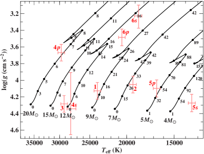
Figure 4: Position of the program stars in a $(T_{\mathrm{eff}},\log(g))$ diagram. Overlaid are evolution tracks for non-rotating stars ($\Omega/\Omega_{\mathrm{crit}}=0$) of metallicity $Z=0.014$ and different initial masses ($M\leq 15\,M_{\sun}$: Georgy et al. 2013; otherwise: Ekström et al. 2012). Black filled circles and numbers mark the age in Myr. Red numbers correspond to those of Table 4. Error bars indicate 99%-confidence limits.

5 Discussion

5.1 Single B- and late O-type stars in Orion

Focusing on a wide range of effective temperatures, we have selected three slow rotators (HD 35299, HD 35912, and HD 37042) from the sample of Nieva & Simón-Díaz (2011) to check our method against previous studies.

As shown in Table 5, our atmospheric parameters have excellent agreement with those derived by Nieva & Simón-Díaz. Similarly, the results for the abundances of helium, carbon, and nitrogen are perfectly consistent with each other within the error bars, even though helium was kept fixed at the solar value in the study of Nieva & Simón-Díaz. The same applies to oxygen and silicon abundances by Simón-Díaz (2010). On the other hand, there are systematic discrepancies apparent for neon, magnesium, and iron that can be attributed either to differences in the synthetic models or in the analysis strategy. For instance, several Mg ii lines, such as $\lambda 4481$ Å have shown to be very sensitive to the replacement of pre-calculated opacity distribution functions, as used by Nieva & Simón-Díaz, with the more flexible concept of opacity sampling that is coherently used here throughout all computational steps, which explains the deviations in magnesium. The disagreements in neon and iron presumably arise from the underlying analysis techniques and in particular from how the microturbulence parameter is constrained. Nevertheless, it is extremely satisfying to see that the results of the two approaches match so well despite being based on contrary conceptional designs.

5.2 Spectroscopic binaries

As a first application to SB2 systems, we have analyzed the composite spectra of three binary systems. While the lines of the two components are sharp and very well separated in our spectrum of HD 119109, the opposite is true for HD 213420 (see Figs. 3a–3). In the case of HD 75821, we have further derived parameters from spectra taken at three distinct orbital phases to investigate its influence on the results.

HD 119109 (#5):

to our knowledge, there is no hint for binarity in the literature for this system so far. Nevertheless, our spectrum shows that this is doubtlessly a SB2 system owing to the many lines that appear twice in the spectrum (see Figs. 3a–3). Given the high quality of our observation and the opportune orbital phase, parameters of both components can be reliably deduced. The system turns out to be composed of two relatively unevolved (see Fig. 4), coeval ($\tau_{\mathrm{p}}=48^{+10}_{-16}\,\mathrm{Myr}$, $\tau_{\mathrm{s}}=49^{+47}_{-48}\,\mathrm{Myr}$) late-type B-stars of masses $M_{\mathrm{p}}=5.2\pm 0.2\,M_{\sun}$ and $M_{\mathrm{s}}=3.5^{+0.4}_{-0.2}\,M_{\sun}$ when using single-star evolutionary tracks. The corresponding squared ratio of radii, $(R_{\star,\mathrm{s}}/R_{\star,\mathrm{p}})^{2}=0.45^{+0.29}_{-0.18}$, is consistent with the surface ratio $A_{\mathrm{eff,s}}/A_{\mathrm{eff,p}}=0.642^{+0.015\mathrm{(stat.)}+0.027\mathrm{(sys.)}}_{-0.013\mathrm{(stat.)}-0.028\mathrm{(sys.)}}$, as is the spectroscopic distance, $d=470^{+70}_{-60}\,\mathrm{pc}$, with the parallax, $\Pi^{-1}=550^{+1700}_{-{\color[rgb]{1,1,1}0}240}\,\mathrm{pc}$. The chemical composition resembles that of the single stars studied in Sect. 5.1.

Using published radial velocity measurements, Tetzlaff et al. (2011) have proposed that this object is a runaway star with high probability based on its peculiar space motion. This conclusion should be considered as uncertain as long as the actual system velocity of this binary is unknown.

HD 213420 (#6):

this well-known binary system with a period of about $880$ days and a radial velocity semi-amplitude of $9\,\mathrm{km\,s^{-1}}$ (Pourbaix et al. 2004) is a clear SB2 system, given the broad absorption features superimposed to He i $\lambda 4438$ Å, $\lambda 6678$ Å, C ii $\lambda 4267$ Å, Mg ii $\lambda 4481$ Å, Si iii $\lambda 4553$ Å, $\lambda 4568$ Å, and S ii $\lambda 5454$ Å (see Figs. 3a–3). Although the signatures of the secondary component are weak and thus only detectable in the case of a high S/N, they are apparently sufficient to determine reasonable atmospheric parameters for the companion because the resulting stellar parameters paint a consistent physical picture: In addition to the finding that the ages of both components (with masses $M_{\mathrm{p}}=10.4^{+1.3}_{-1.2}\,M_{\sun}$, $M_{\mathrm{s}}=11.1^{+0.5}_{-2.1}\,M_{\sun}$) are in perfect agreement ($\tau_{\mathrm{s}}=20^{+10}_{-{\color[rgb]{1,1,1}0}4}\,\mathrm{Myr}$, $\tau_{\mathrm{p}}=18^{+14}_{-{\color[rgb]{1,1,1}0}2}\,\mathrm{Myr}$), the spectroscopic parameter $A_{\mathrm{eff,s}}/A_{\mathrm{eff,p}}=0.936^{+0.014+0.069}_{-0.015-0.060}$ lies within the uncertainty interval of the squared ratio of the evolutionary-track radii, $(R_{\star,\mathrm{s}}/R_{\star,\mathrm{p}})^{2}=1.9^{+1.9}_{-1.1}$. The spectroscopic distance of the system, $d=510^{+110}_{-100}\,\mathrm{pc}$, finally fits to its parallax, $\Pi^{-1}=530^{+210}_{-120}\,\mathrm{pc}$. Apart from a slight tendency to a lower metallicity (see Table 6), the chemical composition agrees with the reference stars of Sect. 5.1.

HD 75821 (#4):

this eclipsing binary has a period of about $26.3$ days and a radial velocity semi-amplitude of $92\,\mathrm{km\,s^{-1}}$ (Mayer et al. 1997).

The spectrum best suited for the spectral analysis is the second one (b) in Table 5, since the spectral line separation is largest in this case, which reveals several pure and unblended features of the companion (see Figs. 3a–3). Reliable atmospheric and stellar parameters for both components are, hence, determinable whereby the latter assume that single-star evolutionary tracks are appropriate. Starting from this premise, the system consists of two coeval components ($\tau_{\mathrm{p}}=7^{+1}_{-1}\,\mathrm{Myr}$, $\tau_{\mathrm{s}}\leq 10\,\mathrm{Myr}$): a massive primary ($M_{\mathrm{p}}=20.2^{+1.8}_{-1.5}\,M_{\sun}$), which is slightly evolved, and a less massive secondary ($M_{\mathrm{s}}=11.5^{+2.0}_{-0.5}\,M_{\sun}$), which is almost unevolved (see Fig. 4). The spectroscopic distance $d=960^{+240}_{-200}\,\mathrm{pc}$ lies well within the 99%-uncertainty range of the parallax, $\Pi^{-1}=1000^{+2300}_{-{\color[rgb]{1,1,1}0}500}\,\mathrm{pc}$. Finally, the spectroscopically deduced effective surface ratio $A_{\mathrm{eff,s}}/A_{\mathrm{eff,p}}=0.218^{+0.003+0.014}_{-0.002-0.011}$ agrees well with the squared ratio of the evolutionary-track radii, $(R_{\star,\mathrm{s}}/R_{\star,\mathrm{p}})^{2}=0.13^{+0.41}_{-0.04}$, and is further consistent with the photometric light curve (Mayer et al. 2014). The elemental abundances of the system are in line with the single stars except for the relatively low helium, nitrogen, and oxygen content (see Table 5).

The heavily blended and, hence, almost vanishing imprints of the companion on the first (a) and third (c) spectrum are insufficient to properly constrain the secondary component’s atmospheric parameters. Instead, unphysical values and large systematic uncertainties, which are induced by variations of $T_{\mathrm{eff}}$ and $\log(g)$ of the primary, are derived for the secondary’s $T_{\mathrm{eff}}$ and $\log(g)$. These error margins are, on the one hand, a direct consequence of strong correlations among certain parameters and, on the other hand, related to the fact that contributions of the secondary component barely affect the spectrum at the corresponding orbital phases. In a simplified picture, increasing the primary’s $T_{\mathrm{eff}}$ and decreasing its $\log(g)$ at the same time causes the He ii lines to become considerably deeper than actually observed, while the He i lines still fit nicely. To compensate for this, $A_{\mathrm{eff,s}}/A_{\mathrm{eff,p}}$ and, hence, the influence of the secondary component, has to be significantly increased to fill the He ii lines with the continuum which thus weakens them again. However, this makes some spectral lines of the secondary component substantially too strong, which, in turn, is corrected for by smearing them out via a larger $\varv\,\sin(i)$ or $\zeta$ that finally leads to a more uncertain determination of $\varv_{\mathrm{rad}}$, given the high degree of line blending at these particular orbital phases.

However, the primary’s properties and the surface ratio $A_{\mathrm{eff,s}}/A_{\mathrm{eff,p}}$ are nicely recovered in all three orbital phases, which gives us confidence that the presented method is generally able to determine them from one single spectrum.

6 Summary

In this paper, a novel objective method to analyze single or composite spectra of early-type stars is presented. It is based on fitting synthetic spectra to observation by using the standard concept of $\chi^{2}$ minimization, which requires the wavelength-dependent noise of the spectrum to be known. Therefore, a simple but precise way of estimating the local noise has been developed (see Sect. 3.1). To facilitate fast and efficient analyses, we make use of pre-calculated grids of synthetic spectra, instead of computing them on demand during the fitting procedure. To sample the entire multi-dimensional parameter space at once, we exploit the unique spectral properties of early-type stars, such as the low density of lines, which reduces the number of models required by several orders of magnitude. In this way, a simultaneous fit of all parameters is possible which has the great advantage that cumbersome iterations by hand or the risk of missing the global best solution are avoided. Moreover, parameters are not only constrained from a subset of available lines but from all useful features in the spectrum. The extension to composite spectra of double-lined binary systems proves extremely valuable in the future, given the high frequency of SB2 systems among early-type stars (see Sana et al. 2012; Chini et al. 2012). In contrast to spectral disentangling techniques like those of Simon & Sturm (1994) or Hadrava (1995), the method presented here allows for – at least – parameters of the primary and the components’ effective surface ratio to be inferred from single-epoch spectra alone.

Statistical and systematic uncertainties of our method are discussed (see Sect. 3.3). The former are based here on a clearly defined mathematical measure, namely the $\chi^{2}$ statistics, while the latter on experience. We show that systematic effects generally dominate in the high-quality regime of our observations. The analysis of a larger sample of stars thus enables us to identify possible shortcomings in our models and to derive results with significantly reduced statistical scatter.

As a case study, we have determined parameters of three well-known stars in the Orion region that turn out to be in excellent agreement with previous studies. Additionally, three binary systems have been analyzed with all of them yielding very conclusive results. Consequently, we are now in a position to homogeneously analyze large samples of early-type stars in relatively short times. The results of a comprehensive investigation of $63$ nearby mid B-type to late O-type stars will be published in a forthcoming paper.

References

• Asplund et al. (2009) Asplund, M., Grevesse, N., Sauval, A. J., & Scott, P. 2009, ARA&A, 47, 481
• Becker (1998) Becker, S. R. 1998, ASP Conf. Ser., 131, 137
• Becker & Butler (1988) Becker, S. R. & Butler, K. 1988, A&A, 201, 232
• Bevington & Robinson (1992) Bevington, P. R. & Robinson, D. K. 1992, Data reduction and error analysis for the physical sciences, 2nd edn. (New York: McGraw-Hill)
• Butler & Giddings (1985) Butler, K. & Giddings, J. R. 1985, in Newsletter of Analysis of Astronomical Spectra, No. 9 (Univ. London)
• Castro et al. (2012) Castro, N., Urbaneja, M. A., Herrero, A., et al. 2012, A&A, 542, A79
• Chini et al. (2012) Chini, R., Hoffmeister, V. H., Nasseri, A., Stahl, O., & Zinnecker, H. 2012, MNRAS, 424, 1925
• Claret & Bloemen (2011) Claret, A. & Bloemen, S. 2011, A&A, 529, A75
• Ducati (2002) Ducati, J. R. 2002, VizieR Online Data Catalog, 2237
• Ekström et al. (2012) Ekström, S., Georgy, C., Eggenberger, P., et al. 2012, A&A, 537, A146
• Frandsen & Lindberg (1999) Frandsen, S. & Lindberg, B. 1999, Astrophysics with the NOT, 71
• Fuhrmann (2008) Fuhrmann, K. 2008, MNRAS, 384, 173
• Georgy et al. (2013) Georgy, C., Ekström, S., Granada, A., et al. 2013, A&A, 553, A24
• Giddings (1981) Giddings, J. R. 1981, PhD thesis, Univ. London
• Gray (2005) Gray, D. F. 2005, The Observation and Analysis of Stellar Photospheres, 3rd edn. (Cambridge: Cambridge University Press)
• Hadrava (1995) Hadrava, P. 1995, A&AS, 114, 393
• Hauck & Mermilliod (1998) Hauck, B. & Mermilliod, M. 1998, A&AS, 129, 431
• Heger & Langer (2000) Heger, A. & Langer, N. 2000, ApJ, 544, 1016
• Høg et al. (2000) Høg, E., Fabricius, C., Makarov, V. V., et al. 2000, A&A, 355, L27
• Houck & Denicola (2000) Houck, J. C. & Denicola, L. A. 2000, in Astronomical Data Analysis Software and Systems IX, eds. N. Manset, C. Veillet, & D. Crabtree, ASP Conf. Ser., 216, 591
• Irrgang et al. (2014) Irrgang, A., Butler, K., Przybilla, N., & Heber, U. 2014, A&A, submitted
• Kaufer et al. (1999) Kaufer, A., Stahl, O., Tubbesing, S., et al. 1999, The Messenger, 95, 8
• Kurucz (1996) Kurucz, R. L. 1996, in Model Atmospheres and Spectrum Synthesis, ed. S. J. Adelman, F. Kupka, & W. W. Weiss (San Francisco: ASP), 160
• Lefever et al. (2010) Lefever, K., Puls, J., Morel, T., et al. 2010, A&A, 515, A74
• Mayer et al. (2014) Mayer, P., Drechsel, H., & Irrgang, A. 2014, A&A, accepted [arXiv:1404.1686]
• Mayer et al. (1997) Mayer, P., Lorenz, R., & Drechsel, H. 1997, A&A, 320, 109
• Mermilliod (1991) Mermilliod, J. C. 1991, Catalogue of Homogeneous Means in the UBV System, Institut d’Astronomie, Universite de Lausanne
• Meynet & Maeder (2000) Meynet, G. & Maeder, A. 2000, A&A, 361, 101
• Mokiem et al. (2005) Mokiem, M. R., de Koter, A., Puls, J., et al. 2005, A&A, 441, 711
• Morel & Butler (2008) Morel, T. & Butler, K. 2008, A&A, 487, 307
• Morel et al. (2006) Morel, T., Butler, K., Aerts, C., Neiner, C., & Briquet, M. 2006, A&A, 457, 651
• Nieva & Przybilla (2006) Nieva, M. F. & Przybilla, N. 2006, ApJ, 639, L39
• Nieva & Przybilla (2007) Nieva, M. F. & Przybilla, N. 2007, A&A, 467, 295
• Nieva & Przybilla (2008) Nieva, M. F. & Przybilla, N. 2008, A&A, 481, 199
• Nieva & Przybilla (2010) Nieva, M.-F. & Przybilla, N. 2010, EAS Publ. Ser., 43, 167
• Nieva & Przybilla (2012) Nieva, M.-F. & Przybilla, N. 2012, A&A, 539, A143
• Nieva & Simón-Díaz (2011) Nieva, M.-F. & Simón-Díaz, S. 2011, A&A, 532, A2
• Palate & Rauw (2012) Palate, M. & Rauw, G. 2012, A&A, 537, A119
• Palate et al. (2013) Palate, M., Rauw, G., Koenigsberger, G., & Moreno, E. 2013, A&A, 552, A39
• Pavlovski & Southworth (2013) Pavlovski, K. & Southworth, J. 2013, arXiv:1312.5261
• Pourbaix et al. (2004) Pourbaix, D., Tokovinin, A. A., Batten, A. H., et al. 2004, A&A, 424, 727
• Przybilla (2005) Przybilla, N. 2005, A&A, 443, 293
• Przybilla (2008) Przybilla, N. 2008, Rev. Mod. Astron., 20, 323
• Przybilla & Butler (2001) Przybilla, N. & Butler, K. 2001, A&A, 379, 955
• Przybilla & Butler (2004) Przybilla, N. & Butler, K. 2004, ApJ, 609, 1181
• Przybilla et al. (2001) Przybilla, N., Butler, K., Becker, S. R., & Kudritzki, R. P. 2001, A&A, 369, 1009
• Przybilla et al. (2006) Przybilla, N., Butler, K., Becker, S. R., & Kudritzki, R. P. 2006, A&A, 445, 1099
• Przybilla et al. (2000) Przybilla, N., Butler, K., Becker, S. R., Kudritzki, R. P., & Venn, K. A. 2000, A&A, 359, 1085
• Przybilla et al. (2011) Przybilla, N., Nieva, M.-F., & Butler, K. 2011, Journal of Physics Conference Series, 328, 012015
• Sana et al. (2012) Sana, H., de Mink, S. E., de Koter, A., et al. 2012, Science, 337, 444
• Sigut (1996) Sigut, T. A. A. 1996, ApJ, 473, 452
• Sigut (1999) Sigut, T. A. A. 1999, ApJ, 519, 303
• Simon & Sturm (1994) Simon, K. P. & Sturm, E. 1994, A&A, 281, 286
• Simón-Díaz (2010) Simón-Díaz, S. 2010, A&A, 510, A22
• Simón-Díaz et al. (2011a) Simón-Díaz, S., Castro, N., Garcia, M., Herrero, A., & Markova, N. 2011a, Bulletin de la Societe Royale des Sciences de Liege, 80, 514
• Simón-Díaz et al. (2011b) Simón-Díaz, S., Castro, N., Herrero, A., et al. 2011b, Journal of Physics Conference Series, 328, 012021
• Smith (1996) Smith, K. C. 1996, Ap&SS, 237, 77
• Tetzlaff et al. (2011) Tetzlaff, N., Neuhäuser, R., & Hohle, M. M. 2011, MNRAS, 410, 190
• van Leeuwen (2007) van Leeuwen, F. 2007, Hipparcos, the New Reduction of the Raw Data (Berlin: Springer), Astrophys. Space Sci. Lib. 350
• Vrancken et al. (1996) Vrancken, M., Butler, K., & Becker, S. R. 1996, A&A, 311, 661