Quantum Teleportation through Noisy Channels with Multi-Qubit GHZ States

Abstract

We investigate two-party quantum teleportation through noisy channels for multi-qubit Greenberger-Horne-Zeilinger (GHZ) states and find which state loses less quantum information in the process. The dynamics of states is described by the master equation with the noisy channels that lead to the quantum channels to be mixed states. We analytically solve the Lindblad equation for $n$-qubit GHZ states $n\in\{4,5,6\}$ where Lindblad operators correspond to the Pauli matrices and describe the decoherence of states. Using the average fidelity we show that 3GHZ state is more robust than $n$GHZ state under most noisy channels. However, $n$GHZ state preserves same quantum information with respect to EPR and 3GHZ states where the noise is in $x$ direction in which the fidelity remains unchanged. We explicitly show that Jung et al. conjecture [Phys. Rev. A 78, 012312 (2008)], namely, “average fidelity with same-axis noisy channels are in general larger than average fidelity with different-axis noisy channels” is not valid for 3GHZ and 4GHZ states.

I Introduction

Quantum teleportation is a process based on classical communication that transmits the quantum information from a location to another with the help of shared quantum entanglement between the sender and receiver. This process is a technique for transporting the state of an atom or photon to the remote recipient even in the absence of quantum communication channels connecting the sender of the quantum state (called Alice) to the recipient (called Bob) nel . The original protocol of this process was firstly introduced by Bennett et al. using the Einstein-Podolsky-Rosen (EPR) state as the quantum channel Bennett93 . Quantum teleportation using two qubit systems is discussed also in chakra10 ; liang13 .

Because of the strong connection between quantum entanglement and quantum teleportation, the usage of multiparticle entangled quantum states other than two-particle entangled states for quantum teleportation has been the subject of various investigations wang07 ; paul11 . In particular, quantum teleportation with three-qubit GHZ state and W state is studied in Refs. karl98 ; wang10 ; gorb03 ; joo03 ; agra06 ; Hu1 . The possibility of teleportation of an unknown qubit using four-particle GHZ state is discussed in Ref. pati00 . It is also shown that the state in the form $|{\psi}\rangle=\frac{1}{\sqrt{2}}\left(|00q_{1}\rangle+|11q_{2}\rangle\right)$ allows perfect two-party teleportation in which $|q_{1}\rangle$ and $|q_{2}\rangle$ are arbitrary normalized single qubit states jung07 .

In quantum information theory and quantum computation, fidelity is a measure to quantify the closeness of two quantum states nel and is closely related to quantum entanglement 4 , quantum phase transitions 6 ; 7 ; 8 , and quantum chaos 5 . Fidelity can be also used to quantify how much quantum information is lost due to noisy channel between initial and final states. This reduction of fidelity is usually due to the interaction of quantum states with environment which results in imperfect teleportation. Thus, the coherence of the entangled state may be lost and it becomes a mixed state. Some efforts have been performed in this direction to realize effective factors which cause this phenomenon Bennett93 ; horodecki99 ; banas01 ; jung08-1 . For instance, Bennett et al. showed that the fidelity of teleportation and the range of accurately teleported states reduce in the less entangled quantum channels Bennett93 .

The existence of noise is an unavoidable property in quantum teleportation process which results is decoherence of states and the reduction of fidelity 0h02 ; han08 ; bhak08 . In particular, Oh et al. using a pair of EPR states showed that the average fidelity and the range of teleported states depend on the type of the noise that acts on the quantum channel and confirmed Bennett et al. results 0h02 . They solved analytically and numerically the master equation with Lindblad structure and found the fidelity as a function of decoherence time and angles of an unknown teleported state.

Note that analytically solving the Lindblad equation in the presence of the noise is not a trivial task in general. Indeed, for multiparticle systems one needs to solve many coupled differential equations that involve tedious computation. For example, for three-particle GHZ state (3GHZ) the master equation reduces to 8 diagonal coupled differential equations and 28 off-diagonal coupled differential equations jung08-2 . The situation is even worse for four-particle GHZ state (4GHZ) that involves 16 diagonal coupled differential equations and 120 off-diagonal coupled differential equations.

In this paper, we analytically solve the master equation for $n$-particle GHZ state ($n\in\{4,5,6\}$) through various noisy channels. The number of coupled differential equations for each case is considerably reduced by using a proper ansatz for the density matrix. The ansatz is determined from the temporal evolution of the initial state of the system. We obtain the fidelity of teleportation and the average fidelity of teleportation that depend on the type of the noisy channel and compare the results with three-particle GHZ state. The goal of this paper is to find out which state is better (loses less quantum information) in the teleportation process with noisy channels. Therefore, although various noisy channels were studied in Ref. 0h02 , we discuss noisy channels which cause the quantum channels to be mixed to compare $n$GHZ states in the process of teleportation.

The organization of this paper is as follows: Section II is devoted to general framework used to evaluate the two-party quantum teleportation circuit. In Sec. III, we analytically solve the Lindblad equation where the quantum channel is a four-particle GHZ state, i.e., $|\mbox{4GHZ}\rangle$. We transmit 4GHZ state through isotropic and Pauli noises and compute the fidelity of teleportation. Moreover, we compare the robustness of 4GHZ state with 3GHZ state in the noisy channels. Solving the master equation for 5GHZ and 6GHZ states when Lindblad operators are in $x$ and $z$ directions is the subject of Secs. IV and V, respectively. We present our conclusions in Sec. VI.

Figure 1: A circuit for quantum teleportation through noisy channels with EPR state. The two top lines belong to Alice and the bottom line to Bob. $M$ denotes measurement and the dotted box represents noisy channel. The Lindblad operator is turned on inside the dotted box.

II GHZ state, fidelity, and Lindblad equation

For $n$-particle system, an $n$GHZ state is a quantum state defined as follows

$$|n\mbox{GHZ}\rangle=\frac{1}{\sqrt{2}}\left(|0\rangle^{\otimes n}+|1\rangle^{\otimes n}\right),$$ (1)

where $n>2$. Note that, teleportation with $|\mbox{EPR}\rangle$ through noisy channels is depicted in Fig. 1 and it is discussed in Ref. 0h02 . Also, teleportation of 3GHZ state through various noisy channels has been previously studied in Ref. jung08-2 . Here, we are interested to investigate the teleportation process for $n$GHZ state through noisy channels for $n\in\{4,5,6\}$. For this purpose, we need to solve the master equation with Lindblad form lind76

$$\frac{\partial\rho}{\partial t}=-\frac{i}{\hbar}[H_{S},\rho]+\sum_{i,\alpha}\left(L_{i,\alpha}\rho L_{i,\alpha}^{\dagger}-\frac{1}{2}\left\{L_{i,\alpha}^{\dagger}L_{i,\alpha},\rho\right\}\right),$$ (2)

in which $L_{i,\alpha}=\sqrt{\kappa_{i,\alpha}}\sigma^{(i)}_{\alpha}$ denote Lindblad operators that describe decoherence and act on the $i$th qubit. Also, $\sigma^{(i)}_{\alpha}$ are the Pauli spin matrices of the $i$th qubit with $\alpha=\{x,y,z\}$, $\kappa_{i,\alpha}$ is the decoherence rate, and $H_{S}$ is the Hamiltonian of the system.

Figure 2: A circuit for quantum teleportation through noisy channels with 4GHZ state. The four top lines belong to Alice and the bottom line to Bob. $M$ denotes measurement and the dotted box represents noisy channel. The Lindblad operator is turned on inside the dotted box.

The unknown state to be teleportated can be written as a Bloch vector on a Bloch sphere

$$|\psi_{\text{in}}\rangle=\cos\left(\frac{\theta}{2}\right)e^{i\phi/2}|0\rangle+\sin\left(\frac{\theta}{2}\right)e^{-i\phi/2}|1\rangle,$$ (3)

where $\theta$ and $\phi$ denote the polar and azimuthal angles, respectively. Fig. 2 shows a quantum teleportation circuit through noisy channels with 4GHZ state in which the input state involves five qubits as the product state of $|\psi_{\text{in}}\rangle$ and $|\mbox{4GHZ}\rangle$. The four top lines (qubits) belong to Alice and bottom one belongs to Bob. The difference of this circuit with the teleportation circuit for EPR state (Fig. 1) is the presence of two more controlled-NOT $\left(\mbox{CNOT}\right)$ gates between $\psi_{\text{in}}$ and 4GHZ states. After measurement of the top four qubits, Bob gets the teleported state $|\psi_{\text{out}}\rangle$. It is convenient to describe the teleportation in terms of the density operator

$$\rho_{\text{out}}=\mbox{Tr}_{1,2,3,4}\left[U_{\mbox{\tiny tel}}\rho_{in}\otimes\varepsilon(\rho_{4\mbox{\tiny GHZ}})U_{\mbox{\tiny tel}}^{\dagger}\right],$$ (4)

where $\rho_{\text{in}}=|\psi_{\text{in}}\rangle\langle\psi_{\text{in}}|$ is density matrix of the unknown initial state and $\varepsilon(\rho_{4\mbox{\tiny GHZ}})$ is the density matrix after transmission through noisy channel which is given by the Lindblad equation. In fact, $\varepsilon$ is a quantum operation that maps $\rho_{4\mbox{\tiny GHZ}}$ to $\varepsilon(\rho_{4\mbox{\tiny GHZ}})$ because of noisy channel and $\rho_{4\mbox{\tiny GHZ}}=|\mbox{4GHZ}\rangle\langle\mbox{4GHZ}|$. Moreover, $U_{\mbox{\tiny tel}}$ is the unitary operator corresponding to the quantum circuit and $\mbox{Tr}_{1,2,3,4}$ is partial trace over first four qubits which belong to Alice.

Fidelity can be used as a tool to measure how much information is lost or preserved through noisy quantum channels in quantum teleportation process. It can be written as the overlap between the input state $|\psi_{in}\rangle$ and the density operator for the teleported state $|\rho_{\text{out}}\rangle$,

$$F=\langle\psi_{\text{in}}|\rho_{\text{out}}|\psi_{\text{in}}\rangle,$$ (5)

that depends on an input state and the type of noise. For the perfect teleportation the fidelity is equal to unity. Also, $1-F$ indicates how much information is lost through the teleportation process. For all possible unknown input states, the average fidelity is given by

$$\overline{}\overline{F}=\frac{1}{4\pi}\int_{0}^{2\pi}\mathrm{d}\phi\int_{0}^{\pi}\mathrm{d}\theta\sin\theta F(\theta,\phi).$$ (6)

Similarly, we find the unitary operator, fidelity and average fidelity for 5GHZ and 6GHZ states in the following sections.

III Four-qubit GHZ state with noisy channels

In this section, we analytically solve the Lindblad equation, Eq. (2), for 4GHZ state through various noisy channels. First, consider $(L_{2,x},L_{3,x},L_{4,x},L_{5,x})$ noise channel with $\kappa_{2,x}=\kappa_{3,x}=\kappa_{4,x}=\kappa_{5,x}=\kappa$ that acts on 4GHZ state. Also, here and throughout the paper we assume $H_{S}=0$.

For this case, the Lindblad equation involves 16 diagonal and 120 off-diagonal coupled linear differential equations which make this equation difficult to be solved analytically. To overcome this problem, we find the time evolution of the density matrix for infinitesimal time interval $\delta t$ using the Lindblad equation as

$$\rho(\delta t)=\rho(0)+\left[\sum_{i,\alpha}\left(L_{i,\alpha}\rho(0)L_{i,\alpha}^{\dagger}\right)-\frac{1}{2}\left\{L_{i,\alpha}^{\dagger}L_{i,\alpha},\rho(0)\right\}\right]\delta t,$$ (7)

where

$$\rho(0)=|\mbox{4GHZ}\rangle\langle\mbox{4GHZ}|=\frac{1}{2}\left[|0\rangle^{\otimes 4}\langle 0|^{\otimes 4}+|0\rangle^{\otimes 4}\langle 1|^{\otimes 4}+|1\rangle^{\otimes 4}\langle 0|^{\otimes 4}+|1\rangle^{\otimes 4}\langle 1|^{\otimes 4}\right].$$ (8)

Substituting $\rho(0)$ in Eq. (7) results in

$$\varepsilon(\rho_{4\mbox{\tiny GHZ}})\Big{|}_{t=\delta t}=\frac{1}{2}{\left(\setcounter{MaxMatrixCols}{14}\begin{smallmatrix}1-4\kappa\delta t&0&0&0&0&0&0&0&0&0&0&0&0&1-4\kappa\delta t\\ 0&\kappa\delta t&0&0&0&0&0&0&0&0&0&0&\kappa\delta t&0\\ 0&0&\kappa\delta t&0&0&0&0&0&0&0&0&\kappa\delta t&0&0\\ 0&0&0&{\footnotesize\tiny1⃝}&0&0&0&0&0&0&{\footnotesize\tiny1⃝}&0&0&0\\ 0&0&0&0&\kappa\delta t&0&0&0&0&\kappa\delta t&0&0&0&0\\ 0&0&0&0&0&{\footnotesize\tiny2⃝}&0&0&{\footnotesize\tiny2⃝}&0&0&0&0&0\\ 0&0&0&0&0&0&\kappa\delta t&\kappa\delta t&0&0&0&0&0&0\\ 0&0&0&0&0&0&\kappa\delta t&\kappa\delta t&0&0&0&0&0&0\\ 0&0&0&0&0&{\footnotesize\tiny2⃝}&0&0&{\footnotesize\tiny2⃝}&0&0&0&0&0\\ 0&0&0&0&\kappa\delta t&0&0&0&0&\kappa\delta t&0&0&0&0\\ 0&0&0&{\footnotesize\tiny1⃝}&0&0&0&0&0&0&{\footnotesize\tiny1⃝}&0&0&0\\ 0&0&\kappa\delta t&0&0&0&0&0&0&0&0&\kappa\delta t&0&0\\ 0&\kappa\delta t&0&0&0&0&0&0&0&0&0&0&\kappa\delta t&0\\ 1-4\kappa\delta t&0&0&0&0&0&0&0&0&0&0&0&0&1-4\kappa\delta t\end{smallmatrix}\right),}$$ (9)

where \emph{n}⃝ denotes $n$ diagonal zeros. Now, because of the form of the density matrix at $t=\delta t$, we use the following ansatz for the density matrix for all times

$$\varepsilon(\rho_{4\mbox{\tiny GHZ}})={\left(\setcounter{MaxMatrixCols}{16}\begin{smallmatrix}a&0&0&0&0&0&0&0&0&0&0&0&0&0&0&a\\ 0&b&0&0&0&0&0&0&0&0&0&0&0&0&b&0\\ 0&0&b&0&0&0&0&0&0&0&0&0&0&b&0&0\\ 0&0&0&c&0&0&0&0&0&0&0&0&c&0&0&0\\ 0&0&0&0&b&0&0&0&0&0&0&b&0&0&0&0\\ 0&0&0&0&0&c&0&0&0&0&c&0&0&0&0&0\\ 0&0&0&0&0&0&c&0&0&c&0&0&0&0&0&0\\ 0&0&0&0&0&0&0&b&b&0&0&0&0&0&0&0\\ 0&0&0&0&0&0&0&b&b&0&0&0&0&0&0&0\\ 0&0&0&0&0&0&c&0&0&c&0&0&0&0&0&0\\ 0&0&0&0&0&c&0&0&0&0&c&0&0&0&0&0\\ 0&0&0&0&b&0&0&0&0&0&0&b&0&0&0&0\\ 0&0&0&c&0&0&0&0&0&0&0&0&c&0&0&0\\ 0&0&b&0&0&0&0&0&0&0&0&0&0&b&0&0\\ 0&b&0&0&0&0&0&0&0&0&0&0&0&0&b&0\\ a&0&0&0&0&0&0&0&0&0&0&0&0&0&0&a\end{smallmatrix}\right).}$$ (10)

Inserting this matrix in the Lindblad equation, Eq. (2), gives us a set of three coupled differential equations

$$\left\{\begin{array}[]{l}\dot{a}(t)=4k\Big{(}b(t)-a(t)\Big{)},\\ \dot{b}(t)=k\Big{(}a(t)-4b(t)+3c(t)\Big{)},\\ \dot{c}(t)=4k\Big{(}b(t)-c(t)\Big{)},\end{array}\right.$$ (14)

subject to the initial conditions $a(0)=1/2$ and $b(0)=c(0)=0$ (see Eq. (8)). The solutions are readily given by

$$\left\{\begin{array}[]{l}a(t)=\frac{1}{16}\left(1+6e^{-4\kappa t}+e^{-8\kappa t}\right),\\ b(t)=\frac{1}{16}\left(1-e^{-8\kappa t}\right),\\ c(t)=\frac{1}{16}\left(1-2e^{-4\kappa t}+e^{-8\kappa t}\right).\end{array}\right.$$ (18)

In fact, the infinitesimal temporal behavior of the density matrix helped us to properly suggest the solution and consequently reduced 136 coupled differential equations to three coupled differential equations which are readily solved. It is now easy to check that $\varepsilon(\rho_{4\mbox{\tiny GHZ}})$, Eq. (10), exactly satisfies the Lindblad equation, Eq. (2), and the validity of the ansatz is verfied.

Having $\varepsilon(\rho_{4\mbox{\tiny GHZ}})$ and $U_{\mbox{\tiny tel}}$ which can be read off from Fig. 2, it is straightforward to compute $\rho_{out}$. Thus, the fidelity reads

$$F(\theta,\phi)=\frac{1}{2}\left[(1+\sin^{2}\theta\cos^{2}\phi)+e^{-4\kappa t}(\cos^{2}\theta+\sin^{2}\theta\sin^{2}\phi)\right],$$ (19)

and the average fidelity is given by

$$\overline{F}=\frac{2}{3}+\frac{1}{3}e^{-4\kappa t}.$$ (20)

Now consider $(L_{2,y},L_{3,y},L_{4,y},L_{5,y})$ and assume $\kappa_{2,y}=\kappa_{3,y}=\kappa_{4,y}=\kappa_{5,y}=\kappa$. Similar to the previous case, using the infinitesimal time evolution of the density matrix

$$\varepsilon(\rho_{4\mbox{\tiny GHZ}})\Big{|}_{t=\delta t}=\frac{1}{2}{\left(\setcounter{MaxMatrixCols}{14}\begin{smallmatrix}1-4\kappa\delta t&0&0&0&0&0&0&0&0&0&0&0&0&1-4\kappa\delta t\\ 0&\kappa\delta t&0&0&0&0&0&0&0&0&0&0&-\kappa\delta t&0\\ 0&0&\kappa\delta t&0&0&0&0&0&0&0&0&-\kappa\delta t&0&0\\ 0&0&0&{\footnotesize\tiny1⃝}&0&0&0&0&0&0&{\footnotesize\tiny1⃝}&0&0&0\\ 0&0&0&0&\kappa\delta t&0&0&0&0&-\kappa\delta t&0&0&0&0\\ 0&0&0&0&0&{\footnotesize\tiny2⃝}&0&0&{\footnotesize\tiny2⃝}&0&0&0&0&0\\ 0&0&0&0&0&0&\kappa\delta t&-\kappa\delta t&0&0&0&0&0&0\\ 0&0&0&0&0&0&-\kappa\delta t&\kappa\delta t&0&0&0&0&0&0\\ 0&0&0&0&0&{\footnotesize\tiny2⃝}&0&0&{\footnotesize\tiny2⃝}&0&0&0&0&0\\ 0&0&0&0&-\kappa\delta t&0&0&0&0&\kappa\delta t&0&0&0&0\\ 0&0&0&{\footnotesize\tiny1⃝}&0&0&0&0&0&0&{\footnotesize\tiny1⃝}&0&0&0\\ 0&0&-\kappa\delta t&0&0&0&0&0&0&0&0&\kappa\delta t&0&0\\ 0&-\kappa\delta t&0&0&0&0&0&0&0&0&0&0&\kappa\delta t&0\\ 1-4\kappa\delta t&0&0&0&0&0&0&0&0&0&0&0&0&1-4\kappa\delta t\end{smallmatrix}\right),}$$ (21)

we take the following ansatz

$$\varepsilon(\rho_{4\mbox{\tiny GHZ}})=\left(\setcounter{MaxMatrixCols}{16}\begin{smallmatrix}a&0&0&0&0&0&0&0&0&0&0&0&0&0&0&a\\ 0&b&0&0&0&0&0&0&0&0&0&0&0&0&-b&0\\ 0&0&b&0&0&0&0&0&0&0&0&0&0&-b&0&0\\ 0&0&0&c&0&0&0&0&0&0&0&0&c&0&0&0\\ 0&0&0&0&b&0&0&0&0&0&0&-b&0&0&0&0\\ 0&0&0&0&0&c&0&0&0&0&c&0&0&0&0&0\\ 0&0&0&0&0&0&c&0&0&c&0&0&0&0&0&0\\ 0&0&0&0&0&0&0&b&-b&0&0&0&0&0&0&0\\ 0&0&0&0&0&0&0&-b&b&0&0&0&0&0&0&0\\ 0&0&0&0&0&0&c&0&0&c&0&0&0&0&0&0\\ 0&0&0&0&0&c&0&0&0&0&c&0&0&0&0&0\\ 0&0&0&0&-b&0&0&0&0&0&0&b&0&0&0&0\\ 0&0&0&c&0&0&0&0&0&0&0&0&c&0&0&0\\ 0&0&-b&0&0&0&0&0&0&0&0&0&0&b&0&0\\ 0&-b&0&0&0&0&0&0&0&0&0&0&0&0&b&0\\ a&0&0&0&0&0&0&0&0&0&0&0&0&0&0&a\end{smallmatrix}\right).$$ (22)

Inserting this matrix in the Lindblad equation, Eq.(2), gives the previous set of coupled differential equations, Eq. (14), and consequently the solutions agree with Eq. (18). For this case the fidelity becomes

$$F(\theta,\phi)=\frac{1}{2}\left[1+(\sin^{2}\theta\sin^{2}\phi+\cos^{2}\theta)e^{-4\kappa t}+\sin^{2}\theta\cos^{2}\phi e^{-8\kappa t}\right],$$ (23)

and the average fidelity reads

$$\overline{F}=\frac{1}{2}+\frac{1}{3}e^{-4\kappa t}+\frac{1}{6}e^{-8\kappa t}.$$ (24)

For the third case consider $(L_{2,z},L_{3,z},L_{4,z},L_{5,z})$ and assume $\kappa_{2,z}=\kappa_{3,z}=\kappa_{4,z}=\kappa_{5,z}=\kappa$. The infinitesimal time evolution of the density matrix gives

$$\varepsilon(\rho_{4\mbox{\tiny GHZ}})\Big{|}_{t=\delta t}=\frac{1}{2}\left(|0\rangle^{\otimes 4}\langle 0|^{\otimes 4}+|1\rangle^{\otimes 4}\langle 1|^{\otimes 4}\right)+\frac{1-8\kappa\delta t}{2}\left(|0\rangle^{\otimes 4}\langle 1|^{\otimes 4}+|1\rangle^{\otimes 4}\langle 0|^{\otimes 4}\right).$$ (25)

So the ansatz is

$$\varepsilon(\rho_{4\mbox{\tiny GHZ}})=a\left(|0\rangle^{\otimes 4}\langle 0|^{\otimes 4}+|1\rangle^{\otimes 4}\langle 1|^{\otimes 4}\right)+b\left(|0\rangle^{\otimes 4}\langle 1|^{\otimes 4}+|1\rangle^{\otimes 4}\langle 0|^{\otimes 4}\right).$$ (26)

Inserting this matrix in the Lindblad equation, Eq. (2), results in

$$\left\{\begin{array}[]{l}\dot{a}(t)=0,\\ \dot{b}(t)=-8k\,b(t),\end{array}\right.$$ (29)

subject to the initial condition $a(0)=b(0)=1/2$. The solution is

$$\varepsilon(\rho_{4\mbox{\tiny GHZ}})=\frac{1}{2}\left(|0\rangle^{\otimes 4}\langle 0|^{\otimes 4}+|1\rangle^{\otimes 4}\langle 1|^{\otimes 4}\right)+\frac{1}{2}e^{-8\kappa t}\left(|0\rangle^{\otimes 4}\langle 1|^{\otimes 4}+|1\rangle^{\otimes 4}\langle 0|^{\otimes 4}\right).$$ (30)

Also, the fidelity and its average read

$$\begin{array}[]{l}\displaystyle F(\theta,\phi)=1-\frac{1}{2}\left(1-e^{-8\kappa t}\right)\sin^{2}\theta,\\ \\ \displaystyle\overline{F}=\frac{2}{3}+\frac{1}{3}e^{-8\kappa t}.\end{array}$$ (34)

The next noisy channel is the isotropic noisy channel. For this case, the master equation involves twelve Lindblad operators $(L_{2,\alpha},L_{3,\alpha},L_{4,\alpha},L_{5,\alpha})$ with $\alpha\in\{x,y,z\}$. At $t=\delta t$ we have

$$\varepsilon(\rho_{4\mbox{\tiny GHZ}})\Big{|}_{t=\delta t}=\frac{1}{2}{\left(\setcounter{MaxMatrixCols}{14}\begin{smallmatrix}1-8\kappa\delta t&0&0&0&0&0&0&0&0&0&0&0&0&1-16\kappa\delta t\\ 0&2\kappa\delta t&0&0&0&0&0&0&0&0&0&0&0&0\\ 0&0&2\kappa\delta t&0&0&0&0&0&0&0&0&0&0&0\\ 0&0&0&{\footnotesize\tiny1⃝}&0&0&0&0&0&0&{\footnotesize\tiny1⃝}&0&0&0\\ 0&0&0&0&2\kappa\delta t&0&0&0&0&0&0&0&0&0\\ 0&0&0&0&0&{\footnotesize\tiny2⃝}&0&0&{\footnotesize\tiny2⃝}&0&0&0&0&0\\ 0&0&0&0&0&0&2\kappa\delta t&0&0&0&0&0&0&0\\ 0&0&0&0&0&0&0&2\kappa\delta t&0&0&0&0&0&0\\ 0&0&0&0&0&{\footnotesize\tiny2⃝}&0&0&{\footnotesize\tiny2⃝}&0&0&0&0&0\\ 0&0&0&0&0&0&0&0&0&2\kappa\delta t&0&0&0&0\\ 0&0&0&{\footnotesize\tiny1⃝}&0&0&0&0&0&0&{\footnotesize\tiny1⃝}&0&0&0\\ 0&0&0&0&0&0&0&0&0&0&0&2\kappa\delta t&0&0\\ 0&0&0&0&0&0&0&0&0&0&0&0&2\kappa\delta t&0\\ 1-16\kappa\delta t&0&0&0&0&0&0&0&0&0&0&0&0&1-8\kappa\delta t\end{smallmatrix}\right).}$$ (35)

So we take the ansatz

$$\varepsilon(\rho_{4\mbox{\tiny GHZ}})=\left(\setcounter{MaxMatrixCols}{16}\begin{smallmatrix}a&0&0&0&0&0&0&0&0&0&0&0&0&0&0&d\\ 0&b&0&0&0&0&0&0&0&0&0&0&0&0&0&0\\ 0&0&b&0&0&0&0&0&0&0&0&0&0&0&0&0\\ 0&0&0&c&0&0&0&0&0&0&0&0&0&0&0&0\\ 0&0&0&0&b&0&0&0&0&0&0&0&0&0&0&0\\ 0&0&0&0&0&c&0&0&0&0&0&0&0&0&0&0\\ 0&0&0&0&0&0&c&0&0&0&0&0&0&0&0&0\\ 0&0&0&0&0&0&0&b&0&0&0&0&0&0&0&0\\ 0&0&0&0&0&0&0&0&b&0&0&0&0&0&0&0\\ 0&0&0&0&0&0&0&0&0&c&0&0&0&0&0&0\\ 0&0&0&0&0&0&0&0&0&0&c&0&0&0&0&0\\ 0&0&0&0&0&0&0&0&0&0&0&b&0&0&0&0\\ 0&0&0&0&0&0&0&0&0&0&0&0&c&0&0&0\\ 0&0&0&0&0&0&0&0&0&0&0&0&0&b&0&0\\ 0&0&0&0&0&0&0&0&0&0&0&0&0&0&b&0\\ d&0&0&0&0&0&0&0&0&0&0&0&0&0&0&a\end{smallmatrix}\right).$$ (36)

Inserting this solution in the Lindblad equation, Eq. (2), we find

$$\left\{\begin{array}[]{l}\dot{a}(t)=8k\Big{(}b(t)-a(t)\Big{)},\\ \dot{b}(t)=2k\Big{(}a(t)-4b(t)+3c(t)\Big{)},\\ \dot{c}(t)=8k\Big{(}b(t)-c(t)\Big{)},\\ \dot{d}(t)=-16k\,d(t),\\ \end{array}\right.$$ (41)

subject to the initial conditions $a(0)=d(0)=1/2$ and $b(0)=c(0)=0$. The solutions are

$$\left\{\begin{array}[]{l}a(t)=\frac{1}{16}\Big{(}1+6e^{-8\kappa t}+e^{-16\kappa t}\Big{)},\\ b(t)=\frac{1}{16}\Big{(}1-e^{-16\kappa t}\Big{)},\\ c(t)=\frac{1}{16}\Big{(}1-2e^{-8\kappa t}+e^{-16\kappa t}\Big{)},\\ d(t)=\frac{1}{2}e^{-16\kappa t}.\end{array}\right.$$ (46)

Also the fidelity is

$$F(\theta,\phi)=\frac{1}{2}\left[1+e^{-8\kappa t}\cos^{2}\theta+e^{-16\kappa t}\sin^{2}\theta\right],$$ (47)

and

$$\overline{F}=\frac{1}{6}\left(3+e^{-8\kappa t}+2e^{-16\kappa t}\right).$$ (48)

To this end, we only considered the noisy channels with the same axis. Now, as a different-axis noisy channel, consider $(L_{2,x},L_{3,y},L_{4,z},L_{5,x})$ noise with $\kappa_{2,x}=\kappa_{3,y}=\kappa_{4,z}=\kappa_{5,x}=\kappa$ that exhibits the effects of noises in different directions. After an infinitesimal time interval and using the Lindblad equation, the density matrix can be written as

$$\varepsilon(\rho_{4\mbox{\tiny GHZ}})\Big{|}_{t=\delta t}=\frac{1}{2}{\left(\setcounter{MaxMatrixCols}{12}\begin{smallmatrix}1-6\kappa\delta t&0&0&0&0&0&0&0&0&0&0&1-10\kappa\delta t\\ 0&\kappa\delta t&0&0&0&0&0&0&0&0&\kappa\delta t&0\\ 0&0&{\footnotesize\tiny2⃝}&0&0&0&0&0&0&{\footnotesize\tiny2⃝}&0&0\\ 0&0&0&\kappa\delta t&0&0&0&0&-\kappa\delta t&0&0&0\\ 0&0&0&0&{\footnotesize\tiny2⃝}&0&0&{\footnotesize\tiny2⃝}&0&0&0&0\\ 0&0&0&0&0&\kappa\delta t&\kappa\delta t&0&0&0&0&0\\ 0&0&0&0&0&\kappa\delta t&\kappa\delta t&0&0&0&0&0\\ 0&0&0&0&{\footnotesize\tiny2⃝}&0&0&{\footnotesize\tiny2⃝}&0&0&0&0\\ 0&0&0&-\kappa\delta t&0&0&0&0&\kappa\delta t&0&0&0\\ 0&0&{\footnotesize\tiny2⃝}&0&0&0&0&0&0&{\footnotesize\tiny2⃝}&0&0\\ 0&\kappa\delta t&0&0&0&0&0&0&0&0&\kappa\delta t&0\\ 1-10\kappa\delta t&0&0&0&0&0&0&0&0&0&0&1-6\kappa\delta t\end{smallmatrix}\right).}$$ (49)

So, the elements of the density matrix for all time can be read off as

$$\varepsilon(\rho_{4\mbox{\tiny GHZ}})=\left(\setcounter{MaxMatrixCols}{16}\begin{smallmatrix}a&0&0&0&0&0&0&0&0&0&0&0&0&0&0&g\\ 0&b&0&0&0&0&0&0&0&0&0&0&0&0&h&0\\ 0&0&c&0&0&0&0&0&0&0&0&0&0&m&0&0\\ 0&0&0&d&0&0&0&0&0&0&0&0&k&0&0&0\\ 0&0&0&0&b&0&0&0&0&0&0&n&0&0&0&0\\ 0&0&0&0&0&d&0&0&0&0&k&0&0&0&0&0\\ 0&0&0&0&0&0&d&0&0&f&0&0&0&0&0&0\\ 0&0&0&0&0&0&0&b&h&0&0&0&0&0&0&0\\ 0&0&0&0&0&0&0&h&b&0&0&0&0&0&0&0\\ 0&0&0&0&0&0&f&0&0&d&0&0&0&0&0&0\\ 0&0&0&0&0&k&0&0&0&0&d&0&0&0&0&0\\ 0&0&0&0&n&0&0&0&0&0&0&b&0&0&0&0\\ 0&0&0&k&0&0&0&0&0&0&0&0&d&0&0&0\\ 0&0&m&0&0&0&0&0&0&0&0&0&0&c&0&0\\ 0&h&0&0&0&0&0&0&0&0&0&0&0&0&b&0\\ g&0&0&0&0&0&0&0&0&0&0&0&0&0&0&a\end{smallmatrix}\right),$$ (50)

which leads to two sets of four and six coupled differential equations, namely

$$\left\{\begin{array}[]{l}\dot{a}(t)=3\kappa\Big{(}b(t)-a(t)\Big{)},\\ \dot{b}(t)=\kappa\Big{(}a(t)-3b(t)+2d(t)\Big{)},\\ \dot{c}(t)=3\kappa\Big{(}d(t)-c(t)\Big{)},\\ \dot{d}(t)=\kappa\Big{(}2b(t)-3d(t)+c(t)\Big{)},\end{array}\right.$$ (55)

and

$$\left\{\begin{array}[]{l}\dot{f}(t)=\kappa\Big{(}-5f(t)+2h(t)-m(t)\Big{)},\\ \dot{g}(t)=\kappa\Big{(}-5g(t)+2h(t)-n(t)\Big{)},\\ \dot{h}(t)=\kappa\Big{(}f(t)+g(t)-5h(t)-k(t)\Big{)},\\ \dot{k}(t)=\kappa\Big{(}-h(t)-5k(t)+m(t)+n(t)\Big{)},\\ \dot{m}(t)=\kappa\Big{(}-f(t)+2k(t)-5m(t)\Big{)},\\ \dot{n}(t)=\kappa\Big{(}-g(t)+2k(t)-5n(t)\Big{)},\end{array}\right.$$ (62)

subject to $a(0)=g(0)=1/2$ and $b(0)=c(0)=d(0)=f(0)=h(0)=k(0)=m(0)=n(0)=0$. The solutions are readily found

$$\left\{\begin{array}[]{l}a(t)=e^{2\kappa t}g(t)=\frac{1}{16}\Big{(}1+3e^{-2\kappa t}+3e^{-4\kappa t}+e^{-6\kappa t}\Big{)},\\ b(t)=e^{2\kappa t}h(t)=-e^{2\kappa t}n(t)=\frac{1}{16}\Big{(}1+e^{-2\kappa t}-e^{-4\kappa t}-e^{-6\kappa t}\Big{)},\\ c(t)=-e^{2\kappa t}m(t)=\frac{1}{16}\Big{(}1-3e^{-2\kappa t}+3e^{-4\kappa t}-e^{-6\kappa t}\Big{)},\\ d(t)=e^{2\kappa t}f(t)=-e^{2\kappa t}k(t)=\frac{1}{16}\Big{(}1-e^{-2\kappa t}-e^{-4\kappa t}+e^{-6\kappa t}\Big{)}.\end{array}\right.$$ (67)

Thus, the fidelity, $F(\theta,\phi)$, and its average, $\overline{F}$, are given by

$$F(\theta,\phi)=\frac{1}{2}\left[1+e^{-2\kappa t}\cos^{2}\theta+e^{-4\kappa t}\sin^{2}\theta\cos^{2}\phi+e^{-6\kappa t}\sin^{2}\theta\sin^{2}\phi\right],$$ (68)

and

$$\overline{F}=\frac{1}{6}\left(3+e^{-2\kappa t}+e^{-4\kappa t}+e^{-6\kappa t}\right).$$ (69)

Table 1: Summary of $F(\theta,\phi)$ and $\overline{F}$ through various noisy channels.

	Noise	3GHZ	4GHZ
	Pauli-X	$\frac{1}{2}\bigg{[}(1+\sin^{2}\theta\cos^{2}\phi$)	$\frac{1}{2}\bigg{[}(1+\sin^{2}\theta\cos^{2}\phi$)
		$+e^{-4\kappa t}(\cos^{2}\theta+\sin^{2}\theta\sin^{2}\phi)\bigg{]}$	$+e^{-4\kappa t}(\cos^{2}\theta+\sin^{2}\theta\sin^{2}\phi)\bigg{]}$
$F(\theta,\phi)$	Pauli-Y	$\frac{1}{2}\bigg{[}1+\sin^{2}\theta\sin^{2}\phi e^{-2\kappa t}+\cos^{2}\theta e^{-4\kappa t}$	$\frac{1}{2}\bigg{[}1+(\sin^{2}\theta\sin^{2}\phi+\cos^{2}\theta)e^{-4\kappa t}$
		$+\sin^{2}\theta\cos^{2}\phi e^{-6\kappa t}\bigg{]}$	$+\sin^{2}\theta\cos^{2}\phi e^{-8\kappa t}\bigg{]}$
	Pauli-Z	$1-\frac{1}{2}(1-e^{-6\kappa t})\sin^{2}\theta$	$1-\frac{1}{2}(1-e^{-8\kappa t})\sin^{2}\theta$
	isotropic	$\frac{1}{2}(1+\cos^{2}\theta e^{-8\kappa t}+\sin^{2}\theta e^{-12\kappa t})$	$\frac{1}{2}(1+\cos^{2}\theta e^{-8\kappa t}+\sin^{2}\theta e^{-16\kappa t})$
	Pauli-X	$\frac{2}{3}+\frac{1}{3}e^{-4\kappa t}$	$\frac{2}{3}+\frac{1}{3}e^{-4\kappa t}$
$\overline{F}$	Pauli-Y	$\frac{1}{6}(3+e^{-2\kappa t}+e^{-4\kappa t}+e^{-6\kappa t})$	$\frac{1}{6}(3+2e^{-4\kappa t}+e^{-8\kappa t})$
	Pauli-Z	$\frac{2}{3}+\frac{1}{3}e^{-6\kappa t}$	$\frac{2}{3}+\frac{1}{3}e^{-8\kappa t}$
	isotropic	$\frac{1}{6}(3+e^{-8\kappa t}+2e^{-12\kappa t})$	$\frac{1}{6}(3+e^{-8\kappa t}+2e^{-16\kappa t})$

In Table 1, a summary of fidelity and average fidelity for 3GHZ jung08-2 and 4GHZ states is reported and compared. Also, their average fidelity versus time is depicted in Fig. 4 for various noisy channels. Comparing 3GHZ and 4GHZ states shows that for $(L_{2,x},L_{3,x},L_{4,x},L_{5,x})$ noise both states have the same fidelity. This result also agrees with Bell state $|\beta_{00}\rangle=\frac{1}{\sqrt{2}}(|00\rangle+|11\rangle)$ 0h02 . However, for other cases 3GHZ state is more robust, i.e., loses less quantum information in the quantum teleportation process with respect to 4GHZ state. Note that, for the isotropic case, the fidelities are approximately equal. These results and those obtained in Refs. jung08-2 ; 0h02 show that increasing the number of qubits can enhance the rate of information lost in quantum teleportation process. Moreover, using a proper ansatz for the density matrix, we reduced the number of coupled differential equations from 136 to at most four coupled equations. Fig. 3 shows average fidelity for 4GHZ state through various noises. As it can be seen from the figure, $(L_{2,x},L_{3,x},L_{4,x},L_{5,x})$ noise does lose less quantum information with respect to others. The next noise with small information lost is $(L_{2,x},L_{3,y},L_{4,z},L_{5,x})$ for $\kappa t<0.2$. However, for $\kappa t>0.2$, $(L_{2,z},L_{3,z},L_{4,z},L_{5,z})$ noise represents a better behavior. Moreover, the isotropic noise and the noise in $y$ direction always result in low fidelity quantum teleportation. In the following sections, we exactly solve the Lindblad equation for 5GHZ and 6GHZ states through two types of noisy channels.

Figure 3: The plot of time dependence of average fidelity through noisy channels for 4GHZ state.

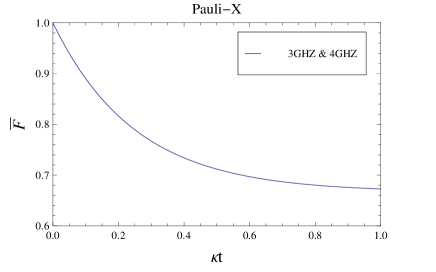
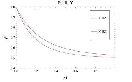
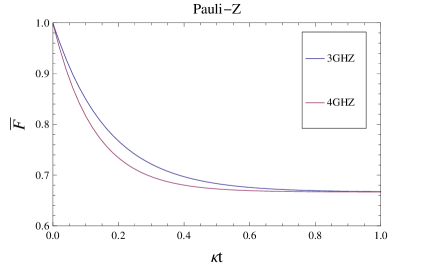
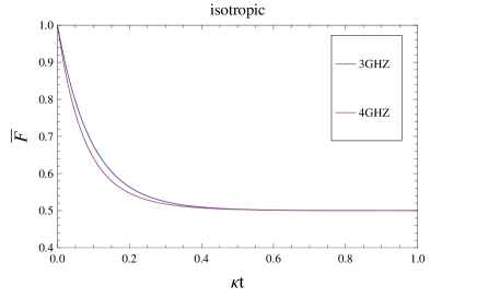
Figure 4: The plot of time dependence of average fidelity for Pauli-X (left up), Pauli-Y (right up), Pauli-Z (left down), and isotropic (right down) noisy channels.

IV Five-qubit GHZ state with noisy channels

In this section, we teleport 5GHZ state through noisy channels as depicted in Fig. 5. For this case the solution of the Lindblad equation is a $32\times 32$ matrix that results in a set of 32 diagonal and 496 off-diagonal coupled differential equations. However, we show that the number of required equations can be considerably reduced by choosing appropriate ansatz for the density matrix.

Figure 5: A circuit for quantum teleportation through noisy channels with 5GHZ state. The five top lines belong to Alice and the bottom line to Bob. $M$ denotes measurement and the dotted box represents noisy channel. The Lindblad operator is turned on inside the dotted box.

First, consider ($L_{2,x}$,$L_{3,x}$,$L_{4,x}$,$L_{5,x}$,$L_{6,x}$) noise and assume $\kappa_{2,x}=\kappa_{3,x}=\kappa_{4,x}=\kappa_{5,x}=\kappa_{6,x}=\kappa$. The infinitesimal time evolution of the density matrix now reads

$$\varepsilon(\rho_{5\mbox{\tiny GHZ}})\Big{|}_{t=\delta t}=\frac{1}{2}{\left(\setcounter{MaxMatrixCols}{18}\begin{smallmatrix}1-5\kappa\delta t&0&0&0&0&0&0&0&0&0&0&0&0&0&0&0&0&1-5\kappa\delta t\\ 0&\kappa\delta t&0&0&0&0&0&0&0&0&0&0&0&0&0&0&\kappa\delta t&0\\ 0&0&\kappa\delta t&0&0&0&0&0&0&0&0&0&0&0&0&\kappa\delta t&0&0\\ 0&0&0&{\footnotesize\tiny1⃝}&0&0&0&0&0&0&0&0&0&0&{\footnotesize\tiny1⃝}&0&0&0\\ 0&0&0&0&\kappa\delta t&0&0&0&0&0&0&0&0&\kappa\delta t&0&0&0&0\\ 0&0&0&0&0&{\footnotesize\tiny3⃝}&0&0&0&0&0&0&0&{\footnotesize\tiny3⃝}&0&0&0&0\\ 0&0&0&0&0&0&\kappa\delta t&0&0&0&0&\kappa\delta t&0&0&0&0&0&0\\ 0&0&0&0&0&0&0&{\footnotesize\tiny6⃝}&0&0&{\footnotesize\tiny6⃝}&0&0&0&0&0&0&0\\ 0&0&0&0&0&0&0&0&\kappa\delta t&\kappa\delta t&0&0&0&0&0&0&0&0\\ 0&0&0&0&0&0&0&0&\kappa\delta t&\kappa\delta t&0&0&0&0&0&0&0&0\\ 0&0&0&0&0&0&0&{\footnotesize\tiny6⃝}&0&0&{\footnotesize\tiny6⃝}&0&0&0&0&0&0&0\\ 0&0&0&0&0&0&\kappa\delta t&0&0&0&0&\kappa\delta t&0&0&0&0&0&0\\ 0&0&0&0&0&{\footnotesize\tiny3⃝}&0&0&0&0&0&0&{\footnotesize\tiny3⃝}&0&0&0&0&0\\ 0&0&0&0&\kappa\delta t&0&0&0&0&0&0&0&0&\kappa\delta t&0&0&0&0\\ 0&0&0&{\footnotesize\tiny1⃝}&0&0&0&0&0&0&0&0&0&0&{\footnotesize\tiny1⃝}&0&0&0\\ 0&0&\kappa\delta t&0&0&0&0&0&0&0&0&0&0&0&0&\kappa\delta t&0&0\\ 0&\kappa\delta t&0&0&0&0&0&0&0&0&0&0&0&0&0&0&\kappa\delta t&0\\ 1-5\kappa\delta t&0&0&0&0&0&0&0&0&0&0&0&0&0&0&0&0&1-5\kappa\delta t\end{smallmatrix}\right).}\hskip 14.22636pt$$ (70)

So we take the ansatz as

$$\varepsilon(\rho_{5\mbox{\tiny GHZ}})=\left(\setcounter{MaxMatrixCols}{18}\begin{smallmatrix}a&0&0&0&0&0&0&0&0&0&0&0&0&0&0&0&0&a\\ 0&b&0&0&0&0&0&0&0&0&0&0&0&0&0&0&b&0\\ 0&0&b&0&0&0&0&0&0&0&0&0&0&0&0&b&0&0\\ 0&0&0&\tiny\emph{c}⃝_{1}&0&0&0&0&0&0&0&0&0&0&\tiny\emph{c}⃝_{1}&0&0&0\\ 0&0&0&0&b&0&0&0&0&0&0&0&0&b&0&0&0&0\\ 0&0&0&0&0&\tiny\emph{c}⃝_{3}&0&0&0&0&0&0&\tiny\emph{c}⃝_{3}&0&0&0&0&0\\ 0&0&0&0&0&0&b&0&0&0&0&b&0&0&0&0&0&0\\ 0&0&0&0&0&0&0&\tiny\emph{c}⃝_{6}&0&0&\tiny\emph{c}⃝_{6}&0&0&0&0&0&0&0\\ 0&0&0&0&0&0&0&0&b&b&0&0&0&0&0&0&0&0\\ 0&0&0&0&0&0&0&0&b&b&0&0&0&0&0&0&0&0\\ 0&0&0&0&0&0&0&\tiny\emph{c}⃝_{6}&0&0&\tiny\emph{c}⃝_{6}&0&0&0&0&0&0&0\\ 0&0&0&0&0&0&b&0&0&0&0&b&0&0&0&0&0&0\\ 0&0&0&0&0&\tiny\emph{c}⃝_{3}&0&0&0&0&0&0&\tiny\emph{c}⃝_{3}&0&0&0&0&0\\ 0&0&0&0&b&0&0&0&0&0&0&0&0&b&0&0&0&0\\ 0&0&0&\tiny\emph{c}⃝_{1}&0&0&0&0&0&0&0&0&0&0&\tiny\emph{c}⃝_{1}&0&0&0\\ 0&0&b&0&0&0&0&0&0&0&0&0&0&0&0&b&0&0\\ 0&b&0&0&0&0&0&0&0&0&0&0&0&0&0&0&b&0\\ a&0&0&0&0&0&0&0&0&0&0&0&0&0&0&0&0&a\end{smallmatrix}\right).\hskip 14.22636pt$$ (71)

Here $\emph{c}⃝_{n}$ denotes $n$ diagonal $c$.

Now inserting this matrix in Lindblad equation, Eq. (2), four coupled differential equations are obtained as follows

$$\left\{\begin{array}[]{l}\dot{a}(t)=5k\Big{(}b(t)-a(t)\Big{)},\\ \dot{b}(t)=k\Big{(}a(t)-5b(t)+4c(t)\Big{)},\\ \dot{c}(t)=2k\Big{(}b(t)-c(t)\Big{)}.\\ \end{array}\right.$$ (75)

Solving this set of equations with the initial conditions $a(0)=1/2$, $b(0)=c(0)=0$, leads to the following solution

$$\left\{\begin{array}[]{l}a(t)=\frac{1}{32}\Big{(}1+10e^{-4\kappa t}+5e^{-8\kappa t}\Big{)},\\ b(t)=\frac{1}{32}\Big{(}1+2e^{-4\kappa t}-3e^{-8\kappa t}\Big{)},\\ c(t)=\frac{1}{32}\Big{(}1-2e^{-4\kappa t}+e^{-8\kappa t}\Big{)}.\end{array}\right.$$ (79)

Substituting $\varepsilon(\rho_{5\mbox{\tiny GHZ}})$ in Eq. (4) and using Eqs. (5) and (6) fidelity and its average are given by

$$F(\theta,\phi) = \frac{1}{2}\left[1+\sin^{2}\theta\cos^{2}\phi+e^{-4\kappa t}(\cos^{2}\theta+\sin^{2}\theta\sin^{2}\phi)\right],$$ (80)

$$\overline{F} = \frac{1}{3}\left(2+e^{-4\kappa t}\right).$$ (81)

For ($L_{2,z}$,$L_{3,z}$,$L_{4,z}$,$L_{5,z}$,$L_{6,z}$) noise with $\kappa_{2,z}=\kappa_{3,z}=\kappa_{4,z}=\kappa_{5,z}=\kappa_{6,z}=\kappa$, the infinitesimal evolution matrix is

$$\varepsilon(\rho_{5\mbox{\tiny GHZ}})\Big{|}_{t=\delta t}=\frac{1}{2}\left(|0\rangle^{\otimes 5}\langle 0|^{\otimes 5}+|1\rangle^{\otimes 5}\langle 1|^{\otimes 5}\right)+\frac{1-10\kappa\delta t}{2}\left(|0\rangle^{\otimes 5}\langle 1|^{\otimes 5}+|1\rangle^{\otimes 5}\langle 0|^{\otimes 5}\right).$$ (82)

Using the ansatz

$$\varepsilon(\rho_{5\mbox{\tiny GHZ}})=a\left(|0\rangle^{\otimes 5}\langle 0|^{\otimes 5}+|1\rangle^{\otimes 5}\langle 1|^{\otimes 5}\right)+b\left(|0\rangle^{\otimes 5}\langle 1|^{\otimes 5}+|1\rangle^{\otimes 5}\langle 0|^{\otimes 5}\right),$$ (83)

we obtain two coupled equations

$$\left\{\begin{array}[]{l}\dot{a}(t)=0,\\ \dot{b}(t)=-10kb(t),\\ \end{array}\right.$$ (86)

subject to $a(0)=1/2$, $b(0)=0$. Therefore, the density matrix reads

$$\varepsilon(\rho_{5\mbox{\tiny GHZ}})=\frac{1}{2}\left(|0\rangle^{\otimes 5}\langle 0|^{\otimes 5}+|1\rangle^{\otimes 5}\langle 1|^{\otimes 5}\right)+\frac{1}{2}e^{-10\kappa t}\left(|0\rangle^{\otimes 5}\langle 1|^{\otimes 5}+|1\rangle^{\otimes 5}\langle 0|^{\otimes 5}\right),$$ (87)

and the fidelity and its average are given by

$$F(\theta,\phi) = 1-\frac{1}{2}\left(1-e^{-10\kappa t}\right)\sin^{2}\theta,$$ (88)

$$\overline{F} = \frac{1}{3}\left(2+e^{-10\kappa t}\right).$$ (89)

V Six-qubit GHZ state with noisy channels

A quantum circuit for teleportation through noisy channels with 6GHZ state is depicted in Fig. 6. In the dotted box the Lindblad operators act on the $64\times 64$ density matrix that involves five Alice’s qubits and one Bob’s qubits. The Lindblad equation, Eq. (2), leads to 64 diagonal and 2016 off-diagonal linear coupled differential equations. However, similar to previous sections, we first study infinitesimal temporal behavior of the density matrix and use a proper ansatz to considerably reduce the number of required equations.

Figure 6: A circuit for quantum teleportation through noisy channels with 6GHZ state. The six top lines belong to Alice and the bottom line to Bob. $M$ denotes measurement and the dotted box represents noisy channel. The Lindblad operator is turned on inside the dotted box.

For ($L_{2,x}$,$L_{3,x}$,$L_{4,x}$,$L_{5,x}$,$L_{6,x},L_{7,x}$) noise and $\kappa_{2,x}=\kappa_{3,x}=\kappa_{4,x}=\kappa_{5,x}=\kappa_{6,x}=\kappa_{7,x}=\kappa$, the Lindblad operators after an infinitesimal time transform the input density matrix $\rho(0)=|6\mbox{GHZ}\rangle\langle 6\mbox{GHZ}|$ to

$$\varepsilon(\rho_{6\mbox{\tiny GHZ}})\Big{|}_{t=\delta t}=\frac{1}{2}\left(\mbox{\footnotesize$\setcounter{MaxMatrixCols}{22}\begin{smallmatrix}1-6\kappa\delta t&0&0&0&0&0&0&0&0&0&0&0&0&0&0&0&0&0&0&0&0&1-6\kappa\delta t\\ 0&\kappa\delta t&0&0&0&0&0&0&0&0&0&0&0&0&0&0&0&0&0&0&\kappa\delta t&0\\ 0&0&\kappa\delta t&0&0&0&0&0&0&0&0&0&0&0&0&0&0&0&0&\kappa\delta t&0&0\\ 0&0&0&{\footnotesize\tiny1⃝}&0&0&0&0&0&0&0&0&0&0&0&0&0&0&{\footnotesize\tiny1⃝}&0&0&0\\ 0&0&0&0&\kappa\delta t&0&0&0&0&0&0&0&0&0&0&0&0&\kappa\delta t&0&0&0&0\\ 0&0&0&0&0&{\footnotesize\tiny3⃝}&0&0&0&0&0&0&0&0&0&0&{\footnotesize\tiny3⃝}&0&0&0&0&0\\ 0&0&0&0&0&0&\kappa\delta t&0&0&0&0&0&0&0&0&\kappa\delta t&0&0&0&0&0&0\\ 0&0&0&0&0&0&0&{\footnotesize\tiny7⃝}&0&0&0&0&0&0&{\footnotesize\tiny7⃝}&0&0&0&0&0&0&0\\ 0&0&0&0&0&0&0&0&\kappa\delta t&0&0&0&0&\kappa\delta t&0&0&0&0&0&0&0&0\\ 0&0&0&0&0&0&0&0&0&{\footnotesize\tiny14⃝}&0&0&{\footnotesize\tiny14⃝}&0&0&0&0&0&0&0&0&0\\ 0&0&0&0&0&0&0&0&0&0&\kappa\delta t&\kappa\delta t&0&0&0&0&0&0&0&0&0&0\\ 0&0&0&0&0&0&0&0&0&0&\kappa\delta t&\kappa\delta t&0&0&0&0&0&0&0&0&0&0\\ 0&0&0&0&0&0&0&0&0&{\footnotesize\tiny14⃝}&0&0&{\footnotesize\tiny14⃝}&0&0&0&0&0&0&0&0&0\\ 0&0&0&0&0&0&0&0&\kappa\delta t&0&0&0&0&\kappa\delta t&0&0&0&0&0&0&0&0\\ 0&0&0&0&0&0&0&{\footnotesize\tiny7⃝}&0&0&0&0&0&0&{\footnotesize\tiny7⃝}&0&0&0&0&0&0&0\\ 0&0&0&0&0&0&\kappa\delta t&0&0&0&0&0&0&0&0&\kappa\delta t&0&0&0&0&0&0\\ 0&0&0&0&0&{\footnotesize\tiny3⃝}&0&0&0&0&0&0&0&0&0&0&{\footnotesize\tiny3⃝}&0&0&0&0&0\\ 0&0&0&0&\kappa\delta t&0&0&0&0&0&0&0&0&0&0&0&0&\kappa\delta t&0&0&0&0\\ 0&0&0&{\footnotesize\tiny1⃝}&0&0&0&0&0&0&0&0&0&0&0&0&0&0&{\footnotesize\tiny1⃝}&0&0&0\\ 0&0&\kappa\delta t&0&0&0&0&0&0&0&0&0&0&0&0&0&0&0&0&\kappa\delta t&0&0\\ 0&\kappa\delta t&0&0&0&0&0&0&0&0&0&0&0&0&0&0&0&0&0&0&\kappa\delta t&0\\ 1-6\kappa\delta t&0&0&0&0&0&0&0&0&0&0&0&0&0&0&0&0&0&0&0&0&1-6\kappa\delta t\end{smallmatrix}$}\right).$$ (90)

So consider the ansatz

$$\varepsilon(\rho_{6\mbox{\tiny GHZ}})=\left(\mbox{\footnotesize$\setcounter{MaxMatrixCols}{48}\begin{smallmatrix}a&0&0&0&0&0&0&0&0&0&0&0&0&0&0&0&0&0&0&0&0&0&0&0&0&0&0&0&0&0&0&0&0&0&0&0&0&0&0&0&0&0&0&0&0&0&0&a\\ 0&b&0&0&0&0&0&0&0&0&0&0&0&0&0&0&0&0&0&0&0&0&0&0&0&0&0&0&0&0&0&0&0&0&0&0&0&0&0&0&0&0&0&0&0&0&b&0\\ 0&0&b&0&0&0&0&0&0&0&0&0&0&0&0&0&0&0&0&0&0&0&0&0&0&0&0&0&0&0&0&0&0&0&0&0&0&0&0&0&0&0&0&0&0&b&0&0\\ 0&0&0&c&0&0&0&0&0&0&0&0&0&0&0&0&0&0&0&0&0&0&0&0&0&0&0&0&0&0&0&0&0&0&0&0&0&0&0&0&0&0&0&0&c&0&0&0\\ 0&0&0&0&b&0&0&0&0&0&0&0&0&0&0&0&0&0&0&0&0&0&0&0&0&0&0&0&0&0&0&0&0&0&0&0&0&0&0&0&0&0&0&b&0&0&0&0\\ 0&0&0&0&0&\tiny\emph{c}⃝&0&0&0&0&0&0&0&0&0&0&0&0&0&0&0&0&0&0&0&0&0&0&0&0&0&0&0&0&0&0&0&0&0&0&0&0&\tiny\emph{c}⃝&0&0&0&0&0\\ 0&0&0&0&0&0&d&0&0&0&0&0&0&0&0&0&0&0&0&0&0&0&0&0&0&0&0&0&0&0&0&0&0&0&0&0&0&0&0&0&0&d&0&0&0&0&0&0\\ 0&0&0&0&0&0&0&b&0&0&0&0&0&0&0&0&0&0&0&0&0&0&0&0&0&0&0&0&0&0&0&0&0&0&0&0&0&0&0&0&b&0&0&0&0&0&0&0\\ 0&0&0&0&0&0&0&0&\tiny\emph{c}⃝&0&0&0&0&0&0&0&0&0&0&0&0&0&0&0&0&0&0&0&0&0&0&0&0&0&0&0&0&0&0&\tiny\emph{c}⃝&0&0&0&0&0&0&0&0\\ 0&0&0&0&0&0&0&0&0&d&0&0&0&0&0&0&0&0&0&0&0&0&0&0&0&0&0&0&0&0&0&0&0&0&0&0&0&0&d&0&0&0&0&0&0&0&0&0\\ 0&0&0&0&0&0&0&0&0&0&c&0&0&0&0&0&0&0&0&0&0&0&0&0&0&0&0&0&0&0&0&0&0&0&0&0&0&c&0&0&0&0&0&0&0&0&0&0\\ 0&0&0&0&0&0&0&0&0&0&0&\tiny\emph{d}⃝&0&0&0&0&0&0&0&0&0&0&0&0&0&0&0&0&0&0&0&0&0&0&0&0&\tiny\emph{d}⃝&0&0&0&0&0&0&0&0&0&0&0\\ 0&0&0&0&0&0&0&0&0&0&0&0&c&0&0&0&0&0&0&0&0&0&0&0&0&0&0&0&0&0&0&0&0&0&0&c&0&0&0&0&0&0&0&0&0&0&0&0\\ 0&0&0&0&0&0&0&0&0&0&0&0&0&b&0&0&0&0&0&0&0&0&0&0&0&0&0&0&0&0&0&0&0&0&b&0&0&0&0&0&0&0&0&0&0&0&0&0\\ 0&0&0&0&0&0&0&0&0&0&0&0&0&0&\tiny\emph{c}⃝&0&0&0&0&0&0&0&0&0&0&0&0&0&0&0&0&0&0&\tiny\emph{c}⃝&0&0&0&0&0&0&0&0&0&0&0&0&0&0\\ 0&0&0&0&0&0&0&0&0&0&0&0&0&0&0&d&0&0&0&0&0&0&0&0&0&0&0&0&0&0&0&0&d&0&0&0&0&0&0&0&0&0&0&0&0&0&0&0\\ 0&0&0&0&0&0&0&0&0&0&0&0&0&0&0&0&c&0&0&0&0&0&0&0&0&0&0&0&0&0&0&c&0&0&0&0&0&0&0&0&0&0&0&0&0&0&0&0\\ 0&0&0&0&0&0&0&0&0&0&0&0&0&0&0&0&0&\tiny\emph{d}⃝&0&0&0&0&0&0&0&0&0&0&0&0&\tiny\emph{d}⃝&0&0&0&0&0&0&0&0&0&0&0&0&0&0&0&0&0\\ 0&0&0&0&0&0&0&0&0&0&0&0&0&0&0&0&0&0&\tiny\emph{c}⃝&0&0&0&0&0&0&0&0&0&0&\tiny\emph{c}⃝&0&0&0&0&0&0&0&0&0&0&0&0&0&0&0&0&0&0\\ 0&0&0&0&0&0&0&0&0&0&0&0&0&0&0&0&0&0&0&\tiny\emph{d}⃝&0&0&0&0&0&0&0&0&\tiny\emph{d}⃝&0&0&0&0&0&0&0&0&0&0&0&0&0&0&0&0&0&0&0\\ 0&0&0&0&0&0&0&0&0&0&0&0&0&0&0&0&0&0&0&0&c&0&0&0&0&0&0&c&0&0&0&0&0&0&0&0&0&0&0&0&0&0&0&0&0&0&0&0\\ 0&0&0&0&0&0&0&0&0&0&0&0&0&0&0&0&0&0&0&0&0&d&0&0&0&0&d&0&0&0&0&0&0&0&0&0&0&0&0&0&0&0&0&0&0&0&0&0\\ 0&0&0&0&0&0&0&0&0&0&0&0&0&0&0&0&0&0&0&0&0&0&\tiny\emph{c}⃝&0&0&\tiny\emph{c}⃝&0&0&0&0&0&0&0&0&0&0&0&0&0&0&0&0&0&0&0&0&0&0\\ 0&0&0&0&0&0&0&0&0&0&0&0&0&0&0&0&0&0&0&0&0&0&0&b&b&0&0&0&0&0&0&0&0&0&0&0&0&0&0&0&0&0&0&0&0&0&0&0\\ 0&0&0&0&0&0&0&0&0&0&0&0&0&0&0&0&0&0&0&0&0&0&0&b&b&0&0&0&0&0&0&0&0&0&0&0&0&0&0&0&0&0&0&0&0&0&0&0\\ 0&0&0&0&0&0&0&0&0&0&0&0&0&0&0&0&0&0&0&0&0&0&\tiny\emph{c}⃝&0&0&\tiny\emph{c}⃝&0&0&0&0&0&0&0&0&0&0&0&0&0&0&0&0&0&0&0&0&0&0\\ 0&0&0&0&0&0&0&0&0&0&0&0&0&0&0&0&0&0&0&0&0&d&0&0&0&0&d&0&0&0&0&0&0&0&0&0&0&0&0&0&0&0&0&0&0&0&0&0\\ 0&0&0&0&0&0&0&0&0&0&0&0&0&0&0&0&0&0&0&0&c&0&0&0&0&0&0&c&0&0&0&0&0&0&0&0&0&0&0&0&0&0&0&0&0&0&0&0\\ 0&0&0&0&0&0&0&0&0&0&0&0&0&0&0&0&0&0&0&\tiny\emph{d}⃝&0&0&0&0&0&0&0&0&\tiny\emph{d}⃝&0&0&0&0&0&0&0&0&0&0&0&0&0&0&0&0&0&0&0\\ 0&0&0&0&0&0&0&0&0&0&0&0&0&0&0&0&0&0&\tiny\emph{c}⃝&0&0&0&0&0&0&0&0&0&0&\tiny\emph{c}⃝&0&0&0&0&0&0&0&0&0&0&0&0&0&0&0&0&0&0\\ 0&0&0&0&0&0&0&0&0&0&0&0&0&0&0&0&0&\tiny\emph{d}⃝&0&0&0&0&0&0&0&0&0&0&0&0&\tiny\emph{d}⃝&0&0&0&0&0&0&0&0&0&0&0&0&0&0&0&0&0\\ 0&0&0&0&0&0&0&0&0&0&0&0&0&0&0&0&c&0&0&0&0&0&0&0&0&0&0&0&0&0&0&c&0&0&0&0&0&0&0&0&0&0&0&0&0&0&0&0\\ 0&0&0&0&0&0&0&0&0&0&0&0&0&0&0&d&0&0&0&0&0&0&0&0&0&0&0&0&0&0&0&0&d&0&0&0&0&0&0&0&0&0&0&0&0&0&0&0\\ 0&0&0&0&0&0&0&0&0&0&0&0&0&0&\tiny\emph{c}⃝&0&0&0&0&0&0&0&0&0&0&0&0&0&0&0&0&0&0&\tiny\emph{c}⃝&0&0&0&0&0&0&0&0&0&0&0&0&0&0\\ 0&0&0&0&0&0&0&0&0&0&0&0&0&b&0&0&0&0&0&0&0&0&0&0&0&0&0&0&0&0&0&0&0&0&b&0&0&0&0&0&0&0&0&0&0&0&0&0\\ 0&0&0&0&0&0&0&0&0&0&0&0&c&0&0&0&0&0&0&0&0&0&0&0&0&0&0&0&0&0&0&0&0&0&0&c&0&0&0&0&0&0&0&0&0&0&0&0\\ 0&0&0&0&0&0&0&0&0&0&0&\tiny\emph{d}⃝&0&0&0&0&0&0&0&0&0&0&0&0&0&0&0&0&0&0&0&0&0&0&0&0&\tiny\emph{d}⃝&0&0&0&0&0&0&0&0&0&0&0\\ 0&0&0&0&0&0&0&0&0&0&c&0&0&0&0&0&0&0&0&0&0&0&0&0&0&0&0&0&0&0&0&0&0&0&0&0&0&c&0&0&0&0&0&0&0&0&0&0\\ 0&0&0&0&0&0&0&0&0&d&0&0&0&0&0&0&0&0&0&0&0&0&0&0&0&0&0&0&0&0&0&0&0&0&0&0&0&0&d&0&0&0&0&0&0&0&0&0\\ 0&0&0&0&0&0&0&0&\tiny\emph{c}⃝&0&0&0&0&0&0&0&0&0&0&0&0&0&0&0&0&0&0&0&0&0&0&0&0&0&0&0&0&0&0&\tiny\emph{c}⃝&0&0&0&0&0&0&0&0\\ 0&0&0&0&0&0&0&b&0&0&0&0&0&0&0&0&0&0&0&0&0&0&0&0&0&0&0&0&0&0&0&0&0&0&0&0&0&0&0&0&b&0&0&0&0&0&0&0\\ 0&0&0&0&0&0&d&0&0&0&0&0&0&0&0&0&0&0&0&0&0&0&0&0&0&0&0&0&0&0&0&0&0&0&0&0&0&0&0&0&0&d&0&0&0&0&0&0\\ 0&0&0&0&0&\tiny\emph{c}⃝&0&0&0&0&0&0&0&0&0&0&0&0&0&0&0&0&0&0&0&0&0&0&0&0&0&0&0&0&0&0&0&0&0&0&0&0&\tiny\emph{c}⃝&0&0&0&0&0\\ 0&0&0&0&b&0&0&0&0&0&0&0&0&0&0&0&0&0&0&0&0&0&0&0&0&0&0&0&0&0&0&0&0&0&0&0&0&0&0&0&0&0&0&b&0&0&0&0\\ 0&0&0&c&0&0&0&0&0&0&0&0&0&0&0&0&0&0&0&0&0&0&0&0&0&0&0&0&0&0&0&0&0&0&0&0&0&0&0&0&0&0&0&0&c&0&0&0\\ 0&0&b&0&0&0&0&0&0&0&0&0&0&0&0&0&0&0&0&0&0&0&0&0&0&0&0&0&0&0&0&0&0&0&0&0&0&0&0&0&0&0&0&0&0&b&0&0\\ 0&b&0&0&0&0&0&0&0&0&0&0&0&0&0&0&0&0&0&0&0&0&0&0&0&0&0&0&0&0&0&0&0&0&0&0&0&0&0&0&0&0&0&0&0&0&b&0\\ a&0&0&0&0&0&0&0&0&0&0&0&0&0&0&0&0&0&0&0&0&0&0&0&0&0&0&0&0&0&0&0&0&0&0&0&0&0&0&0&0&0&0&0&0&0&0&a\\ \end{smallmatrix}$}\right),$$ (91)

where $\small\emph{c}⃝$ and $\small\emph{d}⃝$ denote two diagonal $c$ and $d$, respectively. Substituting this matrix into the Lindblad equation leads to four coupled equations

$$\left\{\begin{array}[]{l}\dot{a}(t)=6k\Big{(}b(t)-a(t)\Big{)},\\ \dot{b}(t)=k\Big{(}a(t)-6b(t)+5c(t)\Big{)},\\ \dot{c}(t)=2k\Big{(}b(t)-3c(t)+2d(t)\Big{)},\\ \dot{d}(t)=-6k\Big{(}c(t)-d(t)\Big{)},\\ \end{array}\right.$$ (96)

subject to $a(0)=1/2$ and $b(0)=c(0)=d(0)=0$. Thus, the solutions read

$$\left\{\begin{array}[]{l}a(t)=\frac{1}{64}\left(1+15e^{-4\kappa t}+15e^{-8\kappa t}+e^{-12\kappa t}\right),\\ b(t)=\frac{1}{64}\left(1+5e^{-4\kappa t}-5e^{-8\kappa t}-e^{-12\kappa t}\right),\\ c(t)=\frac{1}{64}\left(1-e^{-4\kappa t}-e^{-8\kappa t}+e^{-12\kappa t}\right),\\ d(t)=\frac{1}{64}\left(1-3e^{-4\kappa t}+3e^{-8\kappa t}-e^{-12\kappa t}\right),\end{array}\right.$$ (101)

and finally

$$F(\theta,\phi) = \frac{1}{2}\left[1+\sin^{2}\theta\cos^{2}\phi+e^{-4\kappa t}(\cos^{2}\theta+\sin^{2}\theta\sin^{2}\phi)\right],$$ (102)

$$\overline{F} = \frac{1}{3}\left(2+e^{-4\kappa t}\right).$$ (103)

For the last case, we study ($L_{2,z}$,$L_{3,z}$,$L_{4,z}$,$L_{5,z}$,$L_{6,z},L_{7,z}$) noise with $\kappa_{2,z}=\kappa_{3,z}=\kappa_{4,z}=\kappa_{5,z}=\kappa_{6,z}=\kappa_{7,z}=\kappa$. For this case, the temporal evolution matrix is

$$\varepsilon(\rho_{6\mbox{\tiny GHZ}})\Big{|}_{t=\delta t}=\frac{1}{2}\left(|0\rangle^{\otimes 6}\langle 0|^{\otimes 6}+|1\rangle^{\otimes 6}\langle 1|^{\otimes 6}\right)+\frac{1-12\kappa\delta t}{2}\left(|0\rangle^{\otimes 6}\langle 1|^{\otimes 6}+|1\rangle^{\otimes 6}\langle 0|^{\otimes 6}\right),$$ (104)

Therefore, using the ansatz

$$\varepsilon(\rho_{6\mbox{\tiny GHZ}})=a\left(|0\rangle^{\otimes 6}\langle 0|^{\otimes 6}+|1\rangle^{\otimes 6}\langle 1|^{\otimes 6}\right)+b\left(|0\rangle^{\otimes 6}\langle 1|^{\otimes 6}+|1\rangle^{\otimes 6}\langle 0|^{\otimes 6}\right),$$ (105)

we obtain two simple differential equations

$$\left\{\begin{array}[]{l}\dot{a}(t)=0,\\ \dot{b}(t)=-12kb(t),\\ \end{array}\right.$$ (108)

subject to $a(0)=b(0)=1/2$. So the solution is given by

$$\varepsilon(\rho_{6\mbox{\tiny GHZ}})=\frac{1}{2}\left(|0\rangle^{\otimes 6}\langle 0|^{\otimes 6}+|1\rangle^{\otimes 6}\langle 1|^{\otimes 6}\right)+\frac{1}{2}e^{-12\kappa t}\left(|0\rangle^{\otimes 6}\langle 1|^{\otimes 6}+|1\rangle^{\otimes 6}\langle 0|^{\otimes 6}\right),$$ (109)

and the fidelity and its average read

$$F(\theta,\phi) = 1-\frac{1}{2}\left(1-e^{-12\kappa t}\right)\sin^{2}\theta,$$ (110)

$$\overline{F} = \frac{1}{3}\left(2+e^{-12\kappa t}\right).$$ (111)

VI Conclusions

In this paper, we studied quantum teleportation through noisy channels for $n$GHZ states, $n\in\{4,5,6\}$), so that the noisy channels lead to the quantum channels to be mixed states. We exactly solved the Lindblad equation and obtained corresponding density matrices after the transmission process. The Lindblad operators are responsible for the decoherence of quantum states and are defined to be proportional to the Pauli matrices. Solving the Lindblad equation for $n>2$ is not a trivial task in general. For instance, we need to solve 2080 coupled differential equations to find the density matrix for 6GHZ state. We overcame this problem by studying the temporal evolution of the input state and using a proper ansatz for the density matrix. Therefore, we reduced 2080 coupled equations to at most four coupled equations which are readily solved. We found the fidelity and the average fidelity for various cases and showed that for the Lindblad operators corresponding to $x$ direction the fidelity is the same for EPR and $n$GHZ states where $n\in\{3,4,5,6\}$. However, 3GHZ state does lose less quantum information for other types of noisy channel. Note that, In Ref. jung08-2 the authors only studied the same-axis noisy channels and conjectured that “average fidelity with same-axis noisy channels are in general larger than average fidelity with different-axis noisy channels”. However, we showed the failure of this conjecture for 4GHZ state which is apparent in Fig. 3. In the appendix we showed this conjecture also fails for 3GHZ state (see Fig. 7). In fact, for different-axes noises, the analytical solutions can be obtained in the same way, but the number of coupled differential equations usually increases with respect to the same-axes noises.

Appendix A

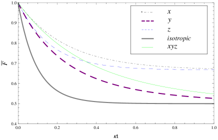
Figure 7: The plot of time dependence of average fidelity for $(L_{2,x},L_{3,y},L_{4,z}$) noisy channels for 3GHZ state.

Here, we present quantum teleportation process through ($L_{2,x},L_{3,y},L_{4,z}$) noisy channel for 3GHZ state which is not studied in Ref. jung08-2 . For this case, the density matrix after $\delta t$ reads

$$\varepsilon(\rho_{3\mbox{\tiny GHZ}})\Big{|}_{t=\delta t}=\frac{1}{2}{\left(\begin{smallmatrix}1-2\kappa\delta t&0&0&0&0&0&0&1-4\kappa\delta t\\ 0&0&0&0&0&0&0&0\\ 0&0&\kappa\delta t&0&0&-\kappa\delta t&0&0\\ 0&0&0&\kappa\delta t&\kappa\delta t&0&0&0\\ 0&0&0&\kappa\delta t&\kappa\delta t&0&0&0\\ 0&0&-\kappa\delta t&0&0&\kappa\delta t&0&0\\ 0&0&0&0&0&0&0&0\\ 1-4\kappa\delta t&0&0&0&0&0&0&1-2\kappa\delta t\end{smallmatrix}\right).}$$ (112)

So, we examine the following ansatz

$$\varepsilon(\rho_{3\mbox{\tiny GHZ}})=\left(\begin{smallmatrix}a&0&0&0&0&0&0&d\\ 0&b&0&0&0&0&e&0\\ 0&0&c&0&0&f&0&0\\ 0&0&0&c&g&0&0&0\\ 0&0&0&g&c&0&0&0\\ 0&0&f&0&0&c&0&0\\ 0&e&0&0&0&0&b&0\\ d&0&0&0&0&0&0&a\end{smallmatrix}\right),$$ (113)

which results in two sets of coupled equations

$$\left\{\begin{array}[]{l}\dot{a}(t)=2k\Big{(}c(t)-a(t)\Big{)},\\ \dot{b}(t)=2k\Big{(}c(t)-b(t)\Big{)},\\ \dot{c}(t)=k\Big{(}a(t)+b(t)-2c(t)\Big{)},\end{array}\right.$$ (117)

and

$$\left\{\begin{array}[]{l}\dot{d}(t)=k\Big{(}g(t)-4d(t)-f(t)\Big{)},\\ \dot{e}(t)=k\Big{(}f(t)-4e(t)-g(t)\Big{)},\\ \dot{f}(t)=k\Big{(}e(t)-d(t)-4f(t)\Big{)},\\ \dot{g}(t)=k\Big{(}d(t)-e(t)-4g(t)\Big{)},\end{array}\right.$$ (122)

subject to $a(0)=d(0)=1/2$ and $b(0)=c(0)=e(0)=f(0)=g(0)=0$. The solutions are

$$\left\{\begin{array}[]{l}a(t)=e^{2\kappa t}d(t)=\frac{1}{8}\Big{(}1+2e^{-2\kappa t}+e^{-4\kappa t}\Big{)},\\ b(t)=-e^{2\kappa t}e(t)=\frac{1}{8}\Big{(}1-2e^{-2\kappa t}+e^{-4\kappa t}\Big{)},\\ c(t)=e^{2\kappa t}g(t)=-e^{2\kappa t}f(t)=\frac{1}{8}\Big{(}1-e^{-4\kappa t}\Big{)}.\end{array}\right.$$ (126)

By using the unitary gate matrix which can be read off from Fig. 2 of Ref. jung08-2 , the fidelity, $F(\theta,\phi)$, and the average fidelity, $\overline{F}$, are given by

$$F(\theta,\phi)=\frac{1}{2}\left[1+e^{-2\kappa t}\left(\cos^{2}\theta+\sin^{2}\theta\sin^{2}\phi\right)+e^{-4\kappa t}\sin^{2}\theta\cos^{2}\phi\right],$$ (127)

and

$$\overline{F}=\frac{1}{6}\left(3+2e^{-2\kappa t}+e^{-4\kappa t}\right).$$ (128)

In Fig. 7, we depicted the average fidelity for 3GHZ state through various noises where the results for the same-axes and isotropic noises are given in Ref. jung08-2 . Therefore, the average fidelity for ($L_{2,x},L_{3,y},L_{4,z}$) noise explicitly contradicts the conjecture proposed by Jung et al. jung08-2 .

References

• (1) M.A. Nielsen and I.L. Chuang, Quantum Computation and Quantum Information (Cambridge University Press, Cambridge, England, 2000).
• (2) C.H. Bennett, G. Brassard, C. Crepeau, R. Jozsa, A. Peres, and W.K. Wootters, Phys. Rev. Lett. 70, 1895 (1993).
• (3) I. Chakrabarty, Eur. Phys. J. D 57, 265 (2010).
• (4) H.-Q. Liang, J.-M. Liu, S.-S. Feng, and J.-G. Chen, Quantum Inf Process 12, 2671 (2013).
• (5) X.-W. Wang, Y.-G. Shan, L.-X. Xia, and M.-W. Lu, Phys. Lett. A 364, 7 (2007).
• (6) N. Paul, J.V. Menon, S. Karumanchi, S. Muralidharan, and P.K. Panigrahi, Quantum. Inf. Process. 10, 619 (2011).
• (7) A. Karlsson and M. Bourennane, Phys. Rev. A 58, 4394 (1998).
• (8) L.-Q. Wang and X.-W. Zha, Opt. Commun. 283, 4118 (2010).
• (9) V.N. Gorbachev, A.A. Rodichkina, and A.I. Truilko, Phys. Lett. A 310, 339 (2003).
• (10) J. Joo, Y-J. Park, S. Oh, and J. Kim, New J. Phys. 5, 136 (2003).
• (11) P. Agrawal and A. Pati, Phys. Rev. A 74, 062320 (2006).
• (12) M.-L. Hu, Phys. Lett. A 375, 922 (2011).
• (13) A.K. Pati, Phys. Rev. A 61, 022308 (2000).
• (14) E. Jung, M. R. Hwang, D. K. Park, J. W. Son, and S. Tamaryan, arXiv:0711.3520.
• (15) Z.H. Ma, F. L. Zhang, D.L. Deng, and J.L. Chen, Phys. Lett. A 373 1616 (2009).
• (16) X. Wang, Z. Sun, and Z.D. Wang, Phys. Rev. A 79, 012105 (2010).
• (17) J. Ma, L. Xu, H. Xiong, and X. Wang, Phys. Rev. E 78, 051126 (2008).
• (18) X.-M. Lu, Z. Sun, X. Wang, and P. Zanardi, Phys. Rev. A 78, 032309 (2008).
• (19) P. Giorda and P. Zanardi, Phys. Rev. E 81, 017203 (2010).
• (20) M. Horodecki, P. Horodocki, and R. Horodocki, Phys. Rev. A 60, 1888 (1999).
• (21) K. Banaszek, Phys. Rev. Lett. 86, 1366 (2001).
• (22) E. Jung, M.R. Hwang, D.K. Park, J.W. Son, and S. Tamaryan, J. Phys. A 41, 385302 (2008).
• (23) S. Oh, S. Lee, and H.W. Lee, Phys. Rev. A 66, 022316 (2002).
• (24) X.P. Han and J.M. Liu, Phys. Scr. 78, 015001 (2008).
• (25) D.D.B. Rao, P.K. Panigrahi, and C. Mitra, Phys. Rev. A 78, 022336 (2008).
• (26) E. Jung, M. R. Hwang, Y.H. Ju, M.S. Kim, S.K. Yoo, H. Kim, D. K. Park, J. W. Son, S. Tamaryan, and S.-K. Cha, Phys. Rev. A 78, 012312 (2008).
• (27) G. Lindblad, Math. Phys. 48, 119 (1976).