On calibration of some distance scales in astrophysics

Abstract

We present a method for distance calibration without using standard fitting procedures. Instead we use random resampling to reconstruct the probability density function (PDF) of calibration data points in the fitting plane. The resulting PDF is then used to estimate distance-related properties. The method is applied to samples of radio surface brightness to diameter ($\Sigma-D$) data for the Galactic supernova remnants (SNRs) and planetary nebulae (PNe), and period-luminosity ($PL$) data for the Large Magellanic Cloud (LMC) fundamental mode classical Cepheids. We argue that resulting density maps can provide more accurate and more reliable calibrations than those obtained by standard linear fitting procedures. For the selected sample of the Galactic SNRs, the presented PDF method of distance calibration results in a smaller average distance fractional error of up to $\approx 16$ percentage points. Similarly, the fractional error is smaller for up to $\approx 8$ and $\approx 0.5$ percentage points, for the samples of Galactic PNe and LMC Cepheids, respectively. In addition, we provide a PDF-based calibration data for each of the samples.

1 Introduction

Scaling relations are widely used, sometimes as the only option, to determine the relevant properties of astrophysical objects. One particularly important property in astrophysical studies is the distance to a particular object. Direct measurement of distances is often not possible, and the only way to infer the distance is from a scaling relation. The calibration of these relations is very important and extensive scientific efforts have been made to assess the quality of the calibration data samples and applied calibration procedures. Most commonly, sample of calibrators is fitted with some analytical functional dependence, where one of the data variables is dependent on one or more remaining data variables. In cases where all data variables have significant uncertainties and cannot be resolved to dependent/independent ones, fitting procedures are adjusted accordingly. If there are $N$ calibrators in a particular calibrating sample, with $n$ coordinates per data point, then there are $n\times N$ numbers of information in that particular calibrating sample. When fitting, all of this information is projected into the linear fit parameters. The initial information contained in the calibration sample is thus reduced and averaged out. While this might not be problematic for the samples with strong functional dependence, in the case of loose correlations (often used in astrophysics) it might cause a significant difference, depending on the type of functional dependence, type of offsets from the best fit line and other assumptions of the applied fitting procedure (Isobe et al., 1990; Urošević et al., 2010; Pavlović et al., 2013).

Modelling kernels based on analytical methods often require that the underlying phenomena appear smooth and predictable. This, however, need not be the case, especially when simplifications are invoked to describe the complexity of the systems with a small number of parameters. This is usually done in studies of astrophysical objects. Evolution of such objects, despite their complex macroscopic appearance, reflected in diversity of intrinsic and environmental parameters, is often described with only two parameters, as is the case with calibration relations considered in this paper. The intrinsic complexity of the nature itself leads to events that cannot be predicted using a simplified analytic approach (Taleb, 2007). Consequently, the shape of the data sample probability density function (PDF) might not follow the direction of the same data sample best fit line and can deviate from that line in Gaussian manner, even in cases of complete and well-studied samples.

Our approach relies on numerical calculation of PDF of calibrating data rather than on applying a fitting procedure to them. This increases the likelihood that the information contained in the calibration sample is preserved and ensures greater consistency and more accurate calibrations.

The standard procedure to estimate PDF from data samples is to bin the data and make histograms. The problem with this approach is that the reconstructed PDFs can heavily depend on the bin size, especially when incomplete calibrating samples are considered (for more information on assessing the binning problem, we refer the reader to Scargle et al., 2013, where a sophisticated approach with Bayesian Blocks method is used). Another possible approach is to reconstruct cumulative distribution function (CDF) and then reconstruct the PDF (Berg & Harris, 2008). However, CDF reconstruction requires data sorting and can only be performed on unidimensional data. Our approach requires no histograms and no CDF reconstruction. We calculate PDF using Monte Carlo resampling of the calibration (original) sample. Coordinates of the data points in resampled samples are translated to account for the difference between centroid coordinates of the original and resampled sample. Our algorithm stems from the basic principles of bootstrap statistics (random resampling, Efron & Tibshirani, 1993) and principal component analysis (standardization of data coordinates using centroids and calculation of highest data variability direction, Pearson, 1901; Jolliffe, 2002). Albeit simple, the algorithm is computationally intensive. However, in present times of ubiquitous computing resources it can be performed with sufficient accuracy on a standard office computer and it can yield smooth PDFs that resemble the distribution of calibration sample data points. Even small samples (of $\sim 10$ data points) can give smooth density maps of high resolution (see Equation 5 and Figure 2). This can be very significant for calibrating relations where scarce samples are a rule rather than exception. We developed our algorithm for the purpose of calibrating bidimensional data samples and our analysis and algorithm presentation will be constrained to two dimensions. The simplicity of our approach makes a multidimensional data application a quite straightforward extension (see Section 2).

We apply our analysis to the radio surface brightness to diameter ($\Sigma-D$) relation for supernova remnants (SNRs) and planetary nebulae (PNe), and also to the period-luminosity ($PL$) relation for classical Cepheids. The majority of the work done on the $\Sigma-D$ relation was in order to produce reliable calibrations that can be used to calculate distances. Samples often suffer from significant scatter and if the information that they contain is described with the parameters of the best fit line, it can result in inaccurate distance estimates. On the other hand, the $PL$ relation gives more consistent distances, with the order of magnitude smaller average fractional error than the above mentioned $\Sigma-D$ relations. The average fractional error for distance is calculated as:

$$\bar{f}=\frac{1}{N}\sum_{i=1}^{N}\left|\frac{d_{\mathrm{i}}-d_{\mathrm{i}}^{\mathrm{s}}}{d_{\mathrm{i}}}\right|,$$ (1)

where $N$ is the number of data points in the calibrating sample, $d_{\mathrm{i}}$ is the measured distance to the object represented with $\mathrm{i}^{\mathrm{th}}$ data point and $d_{\mathrm{i}}^{\mathrm{s}}$ is a statistical distance to that object determined either from the best fit line to the calibrating data set or in some other way such as the PDF-based method presented in this paper.

1.1 The $\Sigma-D$ relations for supernova remnants and planetary nebulae

The relation between the radio surface brightness and diameter is usually given as:

$$\Sigma=AD^{-\beta},$$ (2)

where $A$ and $\beta$ are parameters. This is the standard form that follows from theoretical work (first derived for supernova remnants, Shklovskii, 1960a) and is readily used for calibration. Calibration is performed by linearising the above equation and applying some of the standard fitting techniques (Shklovskii, 1960b). Also, from theoretical considerations it is expected that $A$ and $\beta$ have different values in different stages of SNR evolution and this can also interfere with calibration precision when modelling SNR evolution with only one evolutionary trajectory (the best fit line), which is usually done. Once calibrated, the relation can be used to determine the distance to a particular SNR by measuring its flux density $S=\Sigma/\Omega$ and angular diameter $\theta=\sqrt{4\Omega/\pi}$. After calculating $\Sigma$, the corresponding value for $D$ follows from Equation 2 and distance can be calculated as $d=\theta D$. The $\Sigma-D$ relation for SNRs has more than five decades’ long history. In addition to further theoretical development (i.e., Duric & Seaquist, 1986), extensive work was done on calibrating the relation for distance determination (for some calibrations see, Urošević et al., 2005; Case & Bhattacharya, 1998; Allakhverdiev et al., 1986). The $\Sigma-D$ relation for planetary nebulae in the form of Equation 2 was theoretically derived and empirically assessed by Urošević et al. (2007, 2009).

The above papers use standard fitting procedures based on vertical offsets and are mostly not concerned with further development of fitting procedures. Pavlović et al. (2013) argued that applying different types of fitting offsets can result in different parameters of the $\Sigma-D$ relation for SNRs, and that orthogonal offsets are more reliable and stable over other types of offsets. Similar analysis, but to a lesser extent, was performed on a PNe sample from Stanghellini, Shaw & Villaver (2008) in Vukotić & Urošević (2012). Although these analyses argue in favour of orthogonal offsets calibrations, the dependence of calibration parameters on the type of selected fitting offsets introduces further ambiguities in the efforts towards reliable calibrations. Also, poor quality of the calibrating samples often results in statistically unacceptable fits.

The calibration algorithm proposed in this paper is not using fitting procedures and there are no assumptions on the type of functional dependence in calibrating relation. This makes the resulting calibration more consistent, with no loss of information, because the initial information contained in the data points coordinates is not reduced to the parameters of the best fit line. Here we apply our algorithm for data density distribution calculation to the sample of 60 Galactic SNRs from Pavlović et al. (2013) and to the 39 Galactic PNe with reliable distances from Stanghellini, Shaw & Villaver (2008).

1.2 The $PL$ relation for Cepheids

In the case of Cepheids, pulsating variable stars, historically the period-luminosity relation (Leavitt & Pickering, 1912) was of crucial importance for determining distances. The $PL$ relation is also a starting point of the distance ladder (e.g. Rowan-Robinson, 1985). Using Cepheids to estimate distances to other galaxies is one of the starting points in measuring the Hubble constant ($H_{0}$). Small $PL$ calibration inaccuracies can propagate to significantly larger discrepancies in estimates of the universe expansion rate. As the body of data increased, it became obvious that there are some problems with $PL$ relation, some of which remain unsolved until this day (Sandage & Tammann, 2006). The problems of the $PL$ relation are connected to the problem of reddening in different direction of eyesight, investigation of the metallicity dependence, phase dependency of the relation, universality of the $PL$ relation, or study of the non-linearity of the $PL$ function of various samples (e.g. García-Varela, Sabogal & Ramírez-Tannus, 2013; Kanbur et al., 2010; Koen, Kanbur & Ngeow, 2007). The $PL$ relations in mid infra-red are somewhat less problematic than their visual counterparts, but still, relations at $3.6~{}{\mu}m$ and $4.6~{}{\mu}m$ for samples of Large Magellanic Cloud (LMC) Cepheids (Freedman et al., 2008; Ngeow & Kanbur, 2008; Scowcroft et al., 2011) leave open questions about their metallicity dependency. All of these issues directly affect the estimation of the $H_{0}$.

Studies on the $PL$ relation usually present luminosity in the form of an absolute magnitude $M$ and use $M-\log{P}$ form of the data for plotting and fitting. Once calibrated, the $M-\log{P}$ form can be used as a distance estimation tool. Similarly to the $\Sigma-D$ relation, if the period of a pulsating star is measured, a corresponding $M$ value that is derived from the parameters of the calibration (the line fitted to the calibration sample) can be used to estimate distance $d$ to an object with a measured value of apparent magnitude ($m_{\mathrm{o}}$):

$$d=10^{\left(1.0+\frac{m_{\mathrm{o}}-M}{5.0}\right)}.$$ (3)

We selected the LMC fundamental mode Cepheid samples in I and V band from OGLE project (Soszynski et al., 2008), that was corrected for extinction by Ngeow et al. (2009, and references therein). Compared to the considered samples of Galactic SNRs and PNe, these samples have a significantly larger number of data points (better plotting plane coverage) and should yield more accurate distance calibrations. Also, better accuracy is evident from the smaller scatter in the Cepheid samples relative to the selected axis range, than in the case of SNR and PN samples (scatter of the PDF signal from the best fit line in Figures 2 and 3). Initial conditions and host environments of SNRs and PNe are by far more diverse than for Cepheids and consequently less accurate when described with a single linear relation.

This paper is organized as follows. The next section describes the implementation of our PDF-based algorithm and its features. In Section 3 we present the resulting PDF for selected samples of SNRs, PNe and Cepheids, respectively, and discuss the results. Also, in Table 1 we give the average fractional errors of our calibrations and compare them with previous calibrations while our PDF-based calibrations themselves are given in Tables 2 and 3. Summary of the results and conclusions of this paper are presented in the last section.

2 Method

Rather than fitting the calibration sample we calculate the number density distribution of data points in the 2D fitting plane – which directly relates to probability density distribution of one data variable for the fixed value of the remaining data variable. Our method relies heavily on the philosophy behind bootstrap resampling (Efron & Tibshirani, 1993; Press et al., 2007). Instead of using bootstrap to determine the distribution of the fit parameter values, we used it to estimate the number density distribution of the data points. All of the resampled data samples are plotted against the centroid of the original sample. The coordinates of the resampled data $C={X,Y}$ are calculated as:

$$C=C_{\mathrm{d}}-C_{\mathrm{d}}^{\mathrm{cnt}}+C_{\mathrm{r}}^{\mathrm{cnt}},$$ (4)

where $C_{\mathrm{d}}$ is the corresponding coordinate of the data point, $C_{\mathrm{d}}^{\mathrm{cnt}}$ is the corresponding coordinate of the centroid of the original data sample, while $C_{\mathrm{r}}^{\mathrm{cnt}}$ is the corresponding coordinate of the centroid of the resampled data sample. Our algorithm for the calculation of data points density distribution is as follows:

1. Make a rectangular grid of cells overlayed on the plotting surface.

2. Calculate centroid coordinates for the original data sample and plot the data points.

3. Perform a Monte Carlo resampling with repetition on the original (calibration) data sample to get the resampled sample.

4. Calculate centroid coordinates of the resampled data sample.

5. Calculate plotting coordinates of points in the resampled data sample using Equation 4 and plot them on the same plot as for 1.

6. Repeat steps 2-5 as many times as necessary to get a smooth data point PDF for a given grid resolution.

In the original bootstrap approach, random resampling is used for pinpointing the distribution of fit parameters values. Here we modified this approach (using the SIMD-Oriented Fast Mersenne Twister random number generator, Saito & Matsumoto, 2008) for the purpose of estimating data points number density distribution. The advantage over other mapping techniques is that no binning and smoothing is required. Relevant parameters are contained within the positions of the sample data points. As an example, we present a thought experiment. If we have a sample of several data points that are sufficiently widely spaced, after resampling, each data point would leave a density distribution signal in the form of a “smudge”. The shape of the “smudge” is influenced by the shape of the whole sample, i.e. the most elongated axis of the “smudge” is in the direction of the largest change in the data sample (first principal component). Parts of the plotting plane with high data density will have an overlap of individual “smudges”, shaping the high values part of the data sample PDF (see Figures 2 and 3). Resampling the data sample of just two points gives only three possible resampled samples: first point sampled twice without sampling the second point, second point sampled twice without sampling the first point and both points sampled once. This leaves only three possible centroids and density distribution of poor smoothness. For a sample of $n$ data points it is possible to have:

$$N^{\mathrm{cnt}}=\left(\frac{(2n-1)!}{n!(n-1)!}\right)$$ (5)

different centroids. All of this implies that the quality of the calculated density distribution, in terms of smoothness and resolution, depends on the number of data points in the given sample and their juxtaposition. In all cases we did $10^{6}$ random resamplings and mapped the resulting samples on $10^{2}\times 10^{2}$ or $10^{3}\times 10^{3}$ lattice spanning the coordinates range given in plots from Figures 2 and 3.

After applying the presented algorithm the resulting data sample PDF is in the form of a 2D matrix that can be used as the calibration for distance determination. Instead of using just the fit line (case of fit-based calibrations), one can use the whole PDF matrix that contains much more information about the calibration sample than the line of the best fit to the calibration data. If a fixed value of one variable is selected, than one can normalize the corresponding data sample PDF matrix row or column, in a way that it represents a PDF of the other variable at that particular fixed value of the selected variable. Let us denote with PDF^logΣ=v, a PDF of $D$ at a fixed value $v$ for $\log\Sigma$ and accordingly with PDF^logP=v, a PDF of $M$ at a fixed value $v$ for $\log P$ (in units as in Figures 2 and 3).

To get a single value for the distance to a particular object, SNR, PN, or a Cepheid, it is necessary to get a single value of the desired property of the object from the corresponding PDF distributions ($D$ from PDF^logΣ=v or $m$ from PDF^logP=v). Here, we use basic statistical properties of these distributions for such purpose: mode, mean and median, presented in Tables 2 and 3. Median is the most robust parameter that changes very slowly with data fluctuations and represents the middle value, with equal probability that the value of $D$, or $m$, is situated in higher or lower values than median. This property can be useful in assigning the error bar to the selected diameter (statistical distance) value. Mode marks the value of the highest probability and can be a good estimator of distance for distributions where the corresponding mode peak dominates the whole distribution. Although less stable than median with respect to fluctuations in data, mean value can be useful in estimating error and it describes the resulting PDF in more detail.

2.1 Error estimates for distances to individual objects

The estimation of error in statistical distance derived from the PDF-based method is not trivial and straightforward, since the method gives us a PDF distribution of the statistical distance often not similar to any of the distributions readily used in statistical practice. The error estimate for an individual distance can stem from various reasons: errors in input data values, data sample PDF estimate related errors, errors related to the shapes of PDF^logΣ=v or PDF^logP=v (i.e. data scatter), etc. Errors related to data sample PDF estimate should decrease as the number of resamplings increases, eventually loosing significance compared to other sources of errors. If a data sample PDF is shaped in a Gaussian manner (which is an extremely rare case), the errors related to the shape of PDF^logΣ=v (PDF^logP=v) can be estimated as a Gaussian standard deviation. In the case of irregular shapes, such as the one plotted in Figure 1, the calculation of error estimate may differ from case to case.

The purpose of describing the statistical distribution with an error is to know the probability of a randomly drawn value from that distribution to fall within the error interval. The most frequently used error estimator is the standard deviation, which is the expected value of the variable deviation from the mean. In normal distribution, $68\%$ of the values should be within one standard deviation from the mean. For non-standard distributions this percentage is not known in advance although it can be constrained by means of the Bienaymé-Chebyshev inequality (Dodge, 2008). Instead of making constraints on the percentage of values that are within the error interval, it is better and more precise to calculate them numerically from the PDF. Here, we descriptively present two possibilities:

• Let’s have pointer $l$ pointing to the PDF point which is first to the left hand side of the mode point, and similarly, pointer $r$ pointing to the first next to mode point on the right hand side. Read the values of PDF at points pointed by $l$ and $r$, and denote them with $V_{\mathrm{l}}$ and $V_{\mathrm{r}}$, respectively. Increment the integral sum for the contribution of a higher value, or both values if $V_{\mathrm{l}}=V_{\mathrm{r}}$. Move each pointer that points to the value that was added to the integral sum to the next point in the same direction as before. Repeat this until the integral sum gets larger than a prescribed value, $0.7$, $0.9$, or other. Move one step back the pointer which points to a value whose contribution was not added to the integral sum. The interval between pointers $l$ and $d$ would then represent the error interval for the estimated value that encompasses the desired percentage of variable realizations. This procedure will incorporate parts of variable axis with higher PDF values in the resulting error interval and it should be well-suited for description of error intervals in PDFs with a dominant mode peak (even if wide or asymmetric). This is likely to be the case in stronger correlations.

• Alternatively, one can start from median value and move the pointers in each integration step to the next PDF point in their direction regardless of the $V_{\mathrm{l}}/V_{\mathrm{r}}$ ratio. This will treat in an equal manner both sides of PDF in respect to the median. Since median is a robust estimator, this algorithm might be useful (more realistic) to estimate uncertainties in cases of loose relations.

The two proposed algorithms (or their variations) for error estimates are yet to be developed and tested. Such an extensive work is beyond the scope of this paper and hopefully, in future work, it will be adapted to the specific needs of particular calibrating relations. Future studies and development of the PDF-based calibration methods may give clues on establishing uniform criteria for error estimates on individual distances.

Also, in a PDF-based method, the uncertainties in input values will propagate into PDFs of different shapes. The values of all PDFs corresponding to an input uncertainty interval should be considered as sets of resulting means, medians and modes. The extreme values of elements in these sets indicate the uncertainties interval. These should be combined with the uncertainties caused by the PDF shape, the ones that can be obtained from algorithms (a) and (b), to calculate the final uncertainty (error) of the distance to an individual object.

In the next section, we demonstrate how to use Tables 2 and 3 to get an estimate of the distance to an SNR, a PN or a Cepheid, with a particular example of one selected Galactic SNR, and estimate the uncertainty of this distance by using the corresponding PDF given in Figure 1.

Figure 1: PDF of the diameter variable at the fixed value of $\log{\Sigma}=-19.98$ from the data sample PDF presented in the left panel of Figure 2. Mode, median and mean are presented with dashed, dashed-dotted and dotted lines, respectively. Vertical black solid lines mark one standard deviation confidence interval. Vertical gray lines designate $75\%$ confidence interval around mean, biased towards higher PDF values, as explained in case (a) in Section 2.1. Arrows mark the $75\%$ confidence interval symmetric around median, as stated in case (b) in Section 2.1.

2.2 Distance estimate procedure – the case of SNR G12.0-0.1

The calculation of distance estimate to an SNR using our calibration tables is done in the following steps:

1. From $S$ and $\theta$ calculate $\log\Sigma_{\mathrm{o}}$ of an SNR.

2. Find the $\log\Sigma_{\mathrm{t}}$ value in the calibration table that is the closest match to $\log\Sigma_{\mathrm{o}}$.

3. Use the $D$ values of mode, mean and median (for the PDF${}^{\log\Sigma_{\mathrm{t}}}$) from the $\log\Sigma_{\mathrm{t}}$ table row to calculate distance as $d=D/\theta$. If the distance estimates for mode, mean and median are close together, then mode value should be used as the most probable one. In case where these three estimates differ significantly, an inspection of PDF${}^{\log\Sigma_{\mathrm{t}}}$ may be required, either from a data sample PDF (Figure 2), or directly, as presented in Figure 1. This might be the case for a multi-modal $\log\Sigma_{\mathrm{t}}$ or parts of the plotting plane scarcely populated with data points.

From values presented in Table 3 of Pavlović et al. (2013) we calculate for G12.0-0.1 $\log\Sigma=-19.9686$ (the corresponding PDF^{logΣ=-19.9686} from data PDF in Figure 2 is plotted in Figure 1). The value of ${\log\Sigma=-19.9686}$ falls within the coordinate range of $\log\Sigma=(-20.02,-19.94)$, centred at $\log\Sigma=-19.98$ (corresponding row in Table 2). Similarly, at $10^{3}\times 10^{3}$ resolution (Table 3), the $\log\Sigma=-19.9686$ corresponds to $\log\Sigma=-19.972$ row. From rows corresponding to $\log\Sigma=-19.9686$ in Tables 2 and 3 we read out the $D$ values for mode, mean and median parameters of the PDF^{logΣ=-19.9686}. Inserting $\theta=7^{\prime}$, which is the angular diameter value listed in Table 3 of Pavlović et al. (2013), in $d=D\theta$, we obtain the distance to SNR G12.0-0.1. More precisely, obtained values are $15.5$, $13.5$ and $14.5$ kpc for mode, mean and median at $10^{2}\times 10^{2}$ resolution and $15.2$, $13.7$ and $14.1$ kpc at $10^{3}\times 10^{3}$ resolution, respectively. In Figure 1, the highest PDF peak is dominant and all three estimators are within the range of this peak. In such a case, the most probable value (mode) can be used with high confidence, placing the G12.0-0.1 at the distance of $\sim 15$ kpc. All three estimates are higher than the $\sim 11$ kpc estimate from Pavlović et al. (2013) with the most probable estimates being up to $30\%$ higher. This value is obtained using the same calibrators as in Pavlović et al. (2013) and yet giving a significantly different result.

In the work of Yamauchi, Bamba & Koyama (2013) the authors argue in favour of association of Suzaku X-ray source J181205–1835 with a radio-shell of G12.0-0.1 SNR. They use an X-ray spectra absorption-column-based distance estimate and compare it with distance estimate for G12.0-0.1 obtained from the empirical radio $\Sigma-D$ relation from Pavlović et al. (2013). In this case, the $30\%$ disagreement in $\Sigma-D$ distance estimate can mean the difference of associating and not associating the J181205−1835 source with G12.0-0.1 SNR. When comparing Figure 2 from this paper and Figure 1 from Pavlović et al. (2013), we can see an indication of a densely populated calibrator data point region at $\log\Sigma\sim-20.0$ which is situated to the right of the fit line. This causes the $D$ values estimated from a PDF-based method to be higher than the value estimated from the best line, giving larger distances for a given angular diameter. All of this highlights the importance of local PDF features in statistical distance calibrations that are averaged out in the case of methods based on fitting procedures.

In the case of Cepheids, similarly, the $m$ values (mode, mean and median) corresponding to PDF^logP=v in Tables 2 and 3 are used to calculate $M=m+5(1-\log{d_{\mathrm{LMC}}})$ which is then substituted in Equation 3, along with the corresponding value for $m_{\mathrm{o}}$ in order to calculate the distance estimate (for distance to LMC we used $d_{\mathrm{LMC}}=49970.0$ pc).

As for the error estimates on obtained statistical distances, at $\pm 2\sigma$ ($\sigma$ designating the standard deviation) interval around mean, the Bienaymé-Chebyshev inequality gives that minimum $75\%$ of the diameters should have values inside this interval. However, this constraint is of hardly any use since we integrated that in the case of G12.0-0.1 (Figure 1) $78\%$ of the values are already within $\pm\sigma$ interval (vertical solid black lines in Figure 1). These boundaries correspond to distances of $8.94$ and $20.47$ kpc. Algorithm (a), in favour of higher PDF values, gives $75\%$ confidence interval boundaries at $8.34$ and $17.83$ kpc, plotted with vertical solid gray lines (Figure 1). The same level of confidence for a median-based algorithm (b), plotted with arrows in Figure 1, is from $8.94$ to $23.51$ kpc. As expected, interval from (a), compared to interval from (b) and even to $\pm\sigma$ interval, has the highest PDF value density per unit length of $\log D$ axis and is the narrowest. Even at this, best constrained case at $75\%$ confidence level, the distance uncertainty is $9.49$ kpc, i.e. higher than the lower boundary of the confidence interval. Such a low accuracy (due to a large scatter in the calibrating sample) is of hardly any use for mapping distances, but insight in PDF distributions (such as the one in Figure 1) can be of great use for selecting a fiducial distance estimate (as described in the previous paragraph). The future work on developing methods for integration of confidence intervals and analysis of their span compared to corresponding PDFs, should hopefully result in well-developed algorithms that will be suitable for uniform application to all fixed value PDFs in a 2D PDF matrix and will yield confidence intervals in cases of, for example, values given in Tables 2 and 3.

3 Analysis and Results

Here we present and discuss the resulting PDFs for four selected data samples (Figures 2 and 3). The corresponding $\bar{f}$ values are given in Table 1. The “fit” column values for $\bar{f}$ were calculated using the fit parameters from the references in the corresponding “Sample” column. In the case of SNRs and PNe we selected fit parameters of the procedure that used orthogonal offsets from the best fit line, while in the Cepheid samples the authors fitted the samples with standard $Y(X)$ linear regression using the offsets along the $Y$-axis (this is well-suited since pulsating periods are determined with high precision from OGLE light curves, compared to luminosity, while in the case of $\Sigma-D$ relations for SNRs and PNe there are significant uncertainties in both variables). With the use of standard fit-based calibrations the information contained in the data sample is condensed into the parameters of the fit line along the underlying, fit-related statistical assumptions. While this is helpful in terms of grasping the general evolutionary trends of the data and shorter description of the data sample, it can lead to substantial local inconsistencies when used for distance determination.

Although these local deviations from the fit line are statistically incorporated into the resulting parameters of the calibrating fit, they are often averaged out to a significant degree. Inspection of Figures 2 and 3 and Table 1 shows that PDF-based calibrations are better in tracing the local deviations in the sample, resulting in smaller $\bar{f}$. It follows from Equation 5 that the number of possible different resamplings, in the case of the sample with the smallest number of data points (39 PNe objects), is $\sim 10^{22}$. Selected number of $10^{6}$ resamplings gives enough lattice counts to grasp the significant features of data sample PDF and can be computed with ease on an average desktop computing machine of today. Changing the number of lattice cells from $10^{2}\times 10^{2}$ or $10^{3}\times 10^{3}$ did not significantly change the results (Table 1). The difference between these two cases is smaller than the difference between fit-based and PDF-based calibrations.

Table 1: Average fractional errors in distance determination for calibrating samples fitted in cited works and using the calibration method presented in this paper. Values are given in cases of $10^{2}\times 10^{2}$ and $10^{3}\times 10^{3}$ grid resolution. All values are expressed as percent.

Sample	fit	$10^{2}\times 10^{2}$				$10^{3}\times 10^{3}$
		mode	mean	median		mode	mean	median
SNRs, Pavlović et al. (2013)	47.21	33.15	38.76	35.70		30.60	37.07	35.49
PNe, Vukotić & Urošević (2012)	48.64	44.13	44.33	43.58		40.42	41.72	43.04
Ceph I, Ngeow et al. (2009)	04.85	04.88	04.76	04.88		04.78	04.56	04.46
Ceph V, Ngeow et al. (2009)	07.57	07.72	07.40	07.50		08.00	07.17	07.01

3.1 Galactic SNRs and PNe

In Table 1 the $\bar{f}$ values in “fit” column, taken from Pavlović et al. (2013), were obtained using the orthogonal fit parameters. The PDF of the SNRs sample gives up to $16$ percentage points smaller $\bar{f}$ than in the case of the best fit line. This corresponds to the mode parameter, while median and mean give somewhat larger $\bar{f}$. This implies that the sample is dominated by widely scattered small subsamples of data points (left panel in Figure 2). (A) The first reason for this is that the sample is incomplete and there are unsampled parts of the parameter space populated with every available SNR object out there. In this case, the scatter can be attributed to poorly determined distances of the calibrators that scatter the data points across $\log\Sigma-\log D$ plane. (B) The second explanation is that the sample is sufficiently complete to show out the features of the SNRs real PDF and that diversity and complexity of SNRs evolution cannot be faithfully described only by using $\Sigma$ and $D$ and drawing a single fit line through the calibrating sample. This was pointed out in Arbutina & Urošević (2005) where authors argue that diversity in the density of the SNR surrounding environment can result in SNRs evolving along parallel tracks in the $\Sigma-D$ plane, according to the density of their surroundings. Also, the total energy of the supernovae explosion can be a dominant evolutionary agent in the early stages of SNR evolution, eliminating dependence on the density of the surrounding matter (Berezhko & Völk, 2004). In this scenario, the PDF-based method for distance calibration is much more reliable than just a single fit line-based calibration, as it gets a firmer hold on SNRs complex evolutionary features. For example, if $\Sigma_{\mathrm{o}}$ of particular SNR is measured, its distance can be determined more accurately from a PDF at fixed $\Sigma_{\mathrm{o}}$ along the $D$ coordinate (Figure 1) if the ambient density of the measured SNR $\rho_{\mathrm{o}}$ can be constrained relative to the ambient density of the calibrating SNRs. This will give clues as to which local extreme of the example PDF from Figure 1 can represent the most probable track of the evolution for SNR with $\Sigma_{\mathrm{o}}$ and $\rho_{\mathrm{o}}$ with more accurate SNR distance as a result. In order to strengthen the reasoning from (B), it is of paramount importance that calibrating SNR samples have accurately determined distances, independent of the $\Sigma-D$ relation. Admittedly, this is a huge task, but large future surveys in different parts of the electromagnetic spectrum can give sufficient data for this goal to become feasible.

The general cases of (A) and (B) also hold for the examined PNe sample (Figure 2 and Table 1). Accordingly, a slightly larger $\bar{f}$ than in the case of SNR sample can be attributed either to a smaller number of data points (A) or great diversity in PNe evolution (B). The second case finds good grounds in the work of Frew & Parker (2010) where authors emphasize the diversity of PN properties and different evolutionary scenarios. As in the case of SNRs, larger surveys and data bases will provide more reliable calibrators and give more clues on how to calibrate the $\Sigma-D$ relation.

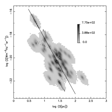
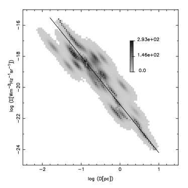
Figure 2: Grayscale reconstructed data PDF. The lattice of $100\times 100$ cells is mapped on the variables range shown on the plot. The markers represent parameters of the distributions at fixed $\Sigma$ values, along the $D$ axis (rows of the plotted PDF matrix): mode – diagonal cross, median – open square and mean – cross. Left: 60 Galactic SNRs sample from Pavlović et al. (2013). Right: 39 Galactic PNe sample from Stanghellini, Shaw & Villaver (2008). Solid line is the orthogonal offsets best fit line with parameters from corresponding works of Pavlović et al. (2013) and Vukotić & Urošević (2012).

3.2 LMC Cepheids

In the case of the Cepheid samples, the PDF-based method gives similar results as the standard fitting method. Somewhat larger values were obtained for estimates from mode parameter in both examined bands and median parameter in I band than for estimates from the fitting method, but smaller $\bar{f}$ for mean parameter in both examined bands and median parameter in V band (Table 1 and Figure 3). The reduction in $\bar{f}$ for V band is larger than in I band and is up to $\approx 0.6$ percentage points (median) and $\approx 0.4$ percentage points (median). This is in agreement with arguments of Section 1.2, that the $PL$ relation in mid infra-red has stronger correlation and is less problematic than in V band. Compared to the samples of SNRs and PNe the Cepheid samples are much more compact and more accurate in terms of $\bar{f}$. This is understandable given that all LMC Cepheids are approximately at the same distance as the host galaxy. It follows that scatter caused by inadequate calibrator distances is much smaller in the case of LMC Cepheids. On the other hand, given the distance ladder propagation of uncertainties, even small improvements in $PL$ calibration can significantly improve accuracy in determining the Hubble parameter.

In addition to potential for providing more precise distance estimates, the more informative nature of the PDF method might give some insight into additional issues of the $PL$ relation for LMC Cepheids (the PDFs from Figure 3). At the $10^{2}\times 10^{2}$ resolution there are not as much distinctive outlying features of the PDF as in the case of SNR and PN samples. Other than that, smaller deviations of markers (that present means, medians and modes at fixed $P$ values along $M$ axis) from the fit line, and their mutual scatter, is evident. This possibility should be more viable especially at higher grid resolution where finer details of the PDF can emerge. Inspection of small deviations of these details and asymmetries from the “central ridge” of the PDF (in an ideal case scenario of the well-fitting model with Gaussian noise, the PDF “central ridge” should be well-defined and symmetric), can help in resolving standard $PL$ issues stated in Section 1.2 and give a more precise insight into the theory of the pulsating nature of these objects. However, it might be a delicate task to distinguish the individual contribution of each of these phenomena to the observed PDF landscape. Interpreting the fine details in PDF shape is beyond the scope of this paper and is left for a future study.

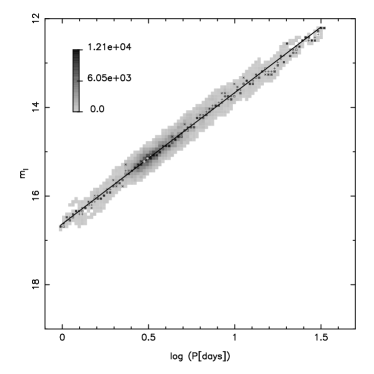
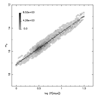
Figure 3: Grayscale reconstructed data PDF for an extinction corrected sample of fundamental mode LMC Cepheids from Ngeow et al. (2009). The lattice of $100\times 100$ cells is mapped on the variables range shown on the plot. The markers represent parameters of the distributions at fixed $P$ values, along the $m$ axis (columns of the plotted PDF matrix): mode – diagonal cross, median – open square and mean – cross. Left: 1649 objects in I band. Right: 1675 objects in V band. Solid line is the vertical offsets best fit line with parameters from corresponding work of Ngeow et al. (2009).

Finally, in Tables 2 and 3 we give distance calibrations from the presented PDF-based method for all three estimators (mode, mean and median) in selected samples of SNRs, PNe and Cepheids. As described in Section 2.2, these calibration tables can be used to estimate distances.

4 Summary and Conclusions

We presented a calibration method which relies on density distribution of data points rather than fitting procedures. The resulting calibrations are more robust and accurate and require no assumptions on functional dependence such as fitting-based calibrations. Our algorithm for generating data sample PDF is based on calculating centroid offsets between Monte Carlo resampled and the actual calibrating data sample. As such, it requires no binning such as in histogram-based approaches. The method is applied to distance related scaling relations, the $\Sigma-D$ relation for SNRs and PNe and the $PL$ relation for Cepheids. The selected samples of Galactic SNRs and PNe have a much larger scatter than selected samples of fundamental mode LMC Cepheids in I and V band. This is due to the fact that Galactic distance mapping is tenuous compared to the case where all objects in the sample reside in external galaxy and are approximately at the same distance. Compared to the best calibrating fit lines for the selected SNRs and PNe, our method gives up to $\approx 16$ and $\approx 8$ percentage points, respectively, smaller average fractional error for distance estimates. Even in the case of LMC Cepheids, a mere fractional error reduction of up to $\approx 0.5$ percentage points can be a significant improvement in building up a Cepheid-based distance ladder.

Apart from improvement in accuracy, the PDF-based calibrating method presented in this paper gives much more information about the data sample than standard fitting techniques. In the proposed method, the information contained in the calibrating samples is preserved rather than averaged out and condensed into the parameters of the best fit line. In the case where data samples are reliable and complete, this preserved information can be used to give more insight into the evolution of the examined objects. This could be a viable tool for quantifying the dependence of the Galactic SNRs evolution on the ambient medium density or some other relevant feature and the same holds for Galactic PNe. In the case of LMC Cepheids, small deviations in a sample PDF can be used to trace the fine details of the nature of pulsations and improvement of the distance ladder.

The main purpose of this paper was to present a more accurate method for statistical distance determination. The more informative nature of the method opens new vistas in giving clues on the evolution of different objects through quantification of sample PDF features. We leave further development of the method in this direction for future work.

Table 2: Calibrating values for distance determination for the Galactic $\Sigma-D$ relations (SNRs and PNe) and the $PL$ relation (in the form of apparent magnitude $m$ vs. period $P$) for fundamental mode Cepheids in I and V band. The units of the $\log$ values and coordinate range are the same as in Figures 2 and 3. The grid size is $10^{2}\times 10^{2}$.

————— SNRs —————				————— PNe —————				—————————– Cepheids —————————–
$\log{\Sigma}$	$D[pc]$			$\log{\Sigma}$	$D[pc]$			$\log{P}$	$m_{\mathrm{I}}$				$m_{\mathrm{V}}$
	mode	mean	med.		mode	mean	med.		mode	mean	med.		mode	mean	med.
-23.42	–	–	–	-24.90	–	–	–	-0.08	–	–	–		–	–	–
-23.34	–	–	–	-24.80	–	–	–	-0.06	–	–	–		–	–	–
-23.26	–	–	–	-24.70	–	–	–	-0.05	–	–	–		–	–	–
-23.18	–	–	–	-24.60	–	–	–	-0.03	–	–	–		–	–	–
-23.10	–	–	–	-24.50	–	–	–	-0.01	16.69	16.69	16.69		17.18	17.18	17.18
-23.02	–	–	–	-24.40	–	–	–	0.01	16.62	16.62	16.69		17.11	17.11	17.18
-22.94	–	–	–	-24.30	–	–	–	0.03	16.48	16.55	16.48		16.97	17.04	16.97
-22.86	44.67	44.67	44.67	-24.20	–	–	–	0.04	16.55	16.48	16.55		17.11	17.04	17.11
-22.78	44.67	41.69	44.67	-24.10	–	–	–	0.06	16.41	16.41	16.48		16.83	16.83	16.90
-22.70	41.69	38.90	41.69	-24.00	7.24	7.94	7.94	0.08	16.34	16.34	16.34		16.83	16.83	16.83
-22.62	38.90	38.90	38.90	-23.90	7.24	7.24	7.94	0.10	16.34	16.41	16.34		16.83	16.90	16.83
-22.54	36.31	36.31	38.90	-23.80	7.24	7.24	7.24	0.12	16.27	16.41	16.34		16.83	16.83	16.83
-22.46	36.31	36.31	36.31	-23.70	6.61	6.61	6.61	0.13	16.27	16.27	16.27		16.69	16.69	16.69
-22.38	33.88	33.88	36.31	-23.60	6.03	6.03	6.03	0.15	16.13	16.13	16.20		16.69	16.69	16.69
-22.30	33.88	33.88	33.88	-23.50	5.50	5.50	6.03	0.17	16.27	16.20	16.13		16.62	16.69	16.62
-22.22	31.62	31.62	31.62	-23.40	5.50	5.50	5.50	0.19	15.99	16.13	16.06		16.41	16.62	16.62
-22.14	31.62	31.62	31.62	-23.30	5.01	5.01	5.01	0.21	16.06	15.99	16.06		16.55	16.55	16.55
-22.06	29.51	29.51	29.51	-23.20	4.57	4.57	4.57	0.22	16.06	16.06	16.06		16.48	16.62	16.62
-21.98	29.51	31.62	29.51	-23.10	4.17	4.17	4.57	0.24	15.99	15.99	15.99		16.48	16.48	16.48
-21.90	15.85	38.90	27.54	-23.00	4.17	4.17	4.17	0.26	15.85	15.92	15.92		16.34	16.41	16.48
-21.82	14.79	44.67	36.31	-22.90	3.80	3.80	3.80	0.28	15.92	15.85	15.92		16.48	16.41	16.48
-21.74	14.79	51.29	67.61	-22.80	3.47	3.47	3.47	0.30	15.64	15.78	15.78		16.20	16.34	16.34
-21.66	165.96	51.29	63.10	-22.70	3.16	3.47	3.47	0.31	15.78	15.71	15.71		16.20	16.20	16.20
-21.58	33.88	51.29	58.88	-22.60	3.16	3.16	3.47	0.33	15.71	15.64	15.71		16.27	16.20	16.27
-21.50	31.62	47.86	54.95	-22.50	3.16	3.16	3.16	0.35	15.78	15.64	15.64		16.41	16.20	16.20
-21.42	31.62	47.86	54.95	-22.40	2.88	2.88	3.16	0.37	15.29	15.43	15.50		15.71	15.99	16.06
-21.34	29.51	47.86	54.95	-22.30	2.88	2.63	2.88	0.39	15.50	15.43	15.50		15.99	15.99	15.99
-21.26	54.95	44.67	54.95	-22.20	2.63	2.19	2.63	0.40	15.43	15.43	15.43		16.06	15.99	15.99
-21.18	54.95	38.90	38.90	-22.10	2.40	1.82	2.40	0.42	15.36	15.36	15.36		15.92	15.92	15.99
-21.10	31.62	33.88	33.88	-22.00	1.05	1.51	1.51	0.44	15.29	15.29	15.36		15.85	15.85	15.92
-21.02	29.51	29.51	31.62	-21.90	0.95	1.38	1.26	0.46	15.22	15.29	15.29		15.78	15.85	15.85
-20.94	29.51	29.51	29.51	-21.80	0.87	1.26	1.15	0.48	15.22	15.22	15.22		15.78	15.78	15.78
-20.86	47.86	29.51	29.51	-21.70	0.87	1.15	1.05	0.49	15.15	15.15	15.15		15.71	15.78	15.78
-20.78	44.67	29.51	33.88	-21.60	0.79	1.05	0.95	0.51	15.08	15.15	15.15		15.71	15.71	15.71
-20.70	41.69	29.51	33.88	-21.50	0.72	0.95	0.87	0.53	15.08	15.08	15.08		15.64	15.71	15.71
-20.62	41.69	29.51	31.62	-21.40	0.66	0.95	0.79	0.55	15.08	15.01	15.08		15.64	15.64	15.64
-20.54	38.90	27.54	29.51	-21.30	0.60	0.87	0.79	0.57	15.01	14.94	15.01		15.50	15.57	15.57
-20.46	25.70	27.54	27.54	-21.20	0.60	0.87	0.95	0.58	14.87	14.87	14.94		15.57	15.50	15.57
-20.38	25.70	27.54	27.54	-21.10	0.95	0.87	0.95	0.60	14.87	14.87	14.87		15.29	15.43	15.50
-20.30	23.99	27.54	25.70	-21.00	0.87	0.79	0.87	0.62	14.87	14.80	14.87		15.57	15.43	15.50
-20.22	22.39	27.54	25.70	-20.90	0.79	0.79	0.87	0.64	14.66	14.73	14.80		15.22	15.36	15.36
-20.14	33.88	29.51	31.62	-20.80	0.79	0.79	0.79	0.66	14.73	14.73	14.73		15.36	15.36	15.36
-20.06	33.88	29.51	31.62	-20.70	0.72	0.72	0.72	0.67	14.66	14.66	14.66		15.22	15.29	15.29
-19.98	31.62	27.54	29.51	-20.60	0.66	0.72	0.79	0.69	14.59	14.59	14.66		15.29	15.29	15.29
-19.90	27.54	27.54	27.54	-20.50	0.79	0.72	0.79	0.71	14.38	14.52	14.52		14.94	15.08	15.15
-19.82	27.54	27.54	27.54	-20.40	0.72	0.72	0.72	0.73	14.45	14.45	14.52		15.15	15.08	15.15
-19.74	25.70	27.54	27.54	-20.30	0.66	0.66	0.66	0.75	14.45	14.38	14.45		15.01	15.01	15.01
-19.66	25.70	27.54	27.54	-20.20	0.60	0.60	0.60	0.76	14.45	14.38	14.45		15.22	15.01	15.08
-19.58	31.62	27.54	29.51	-20.10	0.60	0.55	0.55	0.78	14.24	14.24	14.24		14.87	14.87	14.87
-19.50	29.51	23.99	27.54	-20.00	0.38	0.55	0.50	0.80	14.17	14.24	14.24		14.87	14.87	14.87
-19.42	9.12	20.89	23.99	-19.90	0.35	0.50	0.38	0.82	14.17	14.24	14.24		15.01	14.87	14.94
-19.34	23.99	18.20	22.39	-19.80	0.24	0.46	0.35	0.84	14.17	14.10	14.17		14.80	14.73	14.80
-19.26	9.77	16.98	20.89	-19.70	0.24	0.38	0.35	0.85	14.03	14.03	14.10		14.80	14.66	14.73
-19.18	9.77	14.79	15.85	-19.60	0.29	0.35	0.32	0.87	14.03	13.96	14.03		14.24	14.59	14.59
-19.10	9.77	12.88	14.79	-19.50	0.26	0.32	0.32	0.89	13.96	13.96	13.96		14.52	14.59	14.59

Table 2: – continued

————— SNRs —————				————— PNe —————				—————————– Cepheids —————————–
$\log{\Sigma}$	$D[pc]$			$\log{\Sigma}$	$D[pc]$			$\log{P}$	$m_{\mathrm{I}}$				$m_{\mathrm{V}}$
	mode	mean	med.		mode	mean	med.		mode	mean	med.		mode	mean	med.
-19.02	14.79	9.77	10.47	-19.40	0.42	0.32	0.32	0.91	13.96	13.89	13.96		14.59	14.52	14.59
-18.94	9.77	8.51	9.77	-19.30	0.38	0.29	0.32	0.93	13.68	13.82	13.89		14.87	14.52	14.52
-18.86	4.27	7.41	8.51	-19.20	0.35	0.29	0.32	0.94	13.68	13.75	13.75		14.38	14.38	14.38
-18.78	5.25	6.46	5.62	-19.10	0.35	0.26	0.29	0.96	13.75	13.82	13.75		14.38	14.45	14.45
-18.70	5.25	6.46	5.62	-19.00	0.32	0.22	0.24	0.98	13.82	13.75	13.82		14.59	14.38	14.52
-18.62	10.47	6.92	6.03	-18.90	0.17	0.18	0.20	1.00	13.47	13.68	13.75		14.17	14.38	14.38
-18.54	10.47	7.94	9.77	-18.80	0.15	0.15	0.17	1.02	13.54	13.61	13.61		14.24	14.31	14.31
-18.46	10.47	8.51	10.47	-18.70	0.15	0.13	0.15	1.03	13.68	13.61	13.68		14.45	14.24	14.45
-18.38	9.77	9.77	10.47	-18.60	0.14	0.13	0.14	1.05	13.33	13.47	13.47		14.38	14.10	14.17
-18.30	9.77	10.47	11.22	-18.50	0.14	0.13	0.14	1.07	13.40	13.40	13.40		14.10	14.10	14.17
-18.22	12.02	10.47	11.22	-18.40	0.13	0.14	0.14	1.09	13.47	13.47	13.47		14.24	14.24	14.24
-18.14	11.22	10.47	11.22	-18.30	0.11	0.14	0.14	1.11	13.47	13.40	13.47		14.17	14.10	14.17
-18.06	11.22	10.47	11.22	-18.20	0.11	0.14	0.14	1.12	13.26	13.26	13.33		13.96	14.03	14.03
-17.98	10.47	10.47	11.22	-18.10	0.08	0.14	0.13	1.14	13.33	13.26	13.33		14.10	14.03	14.10
-17.90	10.47	10.47	10.47	-18.00	0.07	0.13	0.10	1.16	13.19	13.19	13.19		13.89	14.03	13.96
-17.82	10.47	10.47	10.47	-17.90	0.07	0.11	0.09	1.18	13.26	13.19	13.12		14.03	13.89	13.89
-17.74	9.77	9.77	10.47	-17.80	0.06	0.10	0.07	1.20	13.26	13.19	13.26		13.89	13.96	13.89
-17.66	9.12	9.12	9.12	-17.70	0.06	0.08	0.07	1.21	13.26	13.19	13.26		13.47	13.89	14.03
-17.58	9.12	9.12	9.12	-17.60	0.05	0.07	0.06	1.23	13.19	13.12	13.19		13.96	13.82	13.96
-17.50	–	–	–	-17.50	0.05	0.06	0.05	1.25	13.05	12.98	13.05		13.82	13.82	13.82
-17.42	6.46	6.92	6.92	-17.40	0.10	0.05	0.05	1.27	12.84	12.91	12.84		13.61	13.68	13.68
-17.34	6.46	6.46	6.46	-17.30	0.09	0.05	0.08	1.29	12.98	12.84	12.98		13.89	13.61	13.68
-17.26	6.03	6.03	6.03	-17.20	0.08	0.05	0.07	1.30	12.56	12.56	12.56		13.89	13.61	13.47
-17.18	6.03	6.03	6.03	-17.10	0.07	0.05	0.07	1.32	12.84	12.70	12.84		13.54	13.47	13.54
-17.10	5.62	5.62	5.62	-17.00	0.07	0.05	0.07	1.34	12.70	12.77	12.77		13.54	13.40	13.54
-17.02	5.62	5.62	5.62	-16.90	0.06	0.05	0.07	1.36	12.77	12.63	12.70		13.26	13.40	13.47
-16.94	5.25	5.25	5.25	-16.80	0.05	0.05	0.06	1.38	12.63	12.63	12.63		13.40	13.33	13.40
-16.86	4.90	4.90	5.25	-16.70	0.05	0.05	0.05	1.39	12.49	12.49	12.49		13.33	13.33	13.33
-16.78	4.90	4.90	4.90	-16.60	0.05	0.05	0.05	1.41	12.42	12.42	12.42		13.47	13.33	13.47
-16.70	4.57	4.57	4.90	-16.50	0.05	0.05	0.05	1.43	12.42	12.49	12.42		12.77	13.05	12.84
-16.62	4.57	4.57	4.57	-16.40	0.04	0.04	0.05	1.45	12.49	12.49	12.49		13.33	13.12	13.12
-16.54	4.57	4.57	4.57	-16.30	0.04	0.04	0.04	1.47	12.49	12.42	12.49		13.05	13.05	13.05
-16.46	4.27	4.27	4.57	-16.20	0.04	0.04	0.04	1.48	12.28	12.35	12.28		13.05	12.84	13.05
-16.38	4.27	4.27	4.27	-16.10	0.03	0.03	0.04	1.50	12.21	12.21	12.21		12.98	12.84	12.98
-16.30	3.98	3.98	3.98	-16.00	0.03	0.03	0.03	1.52	12.21	12.21	12.21		–	–	–
-16.22	3.72	3.98	3.72	-15.90	0.03	0.03	0.03	1.54	–	–	–		–	–	–
-16.14	–	–	–	-15.80	0.03	0.03	0.03	1.56	–	–	–		–	–	–
-16.06	–	–	–	-15.70	0.03	0.03	0.03	1.57	–	–	–		–	–	–
-15.98	–	–	–	-15.60	0.03	0.03	0.03	1.59	–	–	–		–	–	–
-15.90	–	–	–	-15.50	–	–	–	1.61	–	–	–		–	–	–
-15.82	–	–	–	-15.40	–	–	–	1.63	–	–	–		–	–	–
-15.74	–	–	–	-15.30	–	–	–	1.65	–	–	–		–	–	–
-15.66	–	–	–	-15.20	–	–	–	1.66	–	–	–		–	–	–
-15.58	–	–	–	-15.10	–	–	–	1.68	–	–	–		–	–	–

Table 3: Calibrating values for distance determination for the Galactic $\Sigma-D$ relations (SNRs and PNe) and the $PL$ relation (in the form of apparent magnitude $m$ vs. period $P$) for fundamental mode Cepheids in I and V band. The units of the $\log$ values and coordinate range are the same as in Figures 2 and 3. The grid size is $10^{3}\times 10^{3}$. The complete table is available as an on-line material.

————— SNRs —————

————— PNe —————

—————————– Cepheids —————————–

$\log{\Sigma}$

$D[pc]$

$\log{\Sigma}$

$D[pc]$

$\log{P}$

$m_{\mathrm{I}}$

$m_{\mathrm{V}}$

mode

mean

med.

mode

mean

med.

mode

mean

med.

mode

mean

med.

-23.492

–

–

–

-24.990

–

–

–

-0.0982

–

–

–

–

–

–

-23.484

–

–

–

-24.980

–

–

–

-0.0964

–

–

–

–

–

–

-23.476

–

–

–

-24.970

–

–

–

-0.0946

–

–

–

–

–

–

-23.468

–

–

–

-24.960

–

–

–

-0.0928

–

–

–

–

–

–

-23.460

–

–

–

-24.950

–

–

–

-0.0910

–

–

–

–

–

–

-23.452

–

–

–

-24.940

–

–

–

-0.0892

–

–

–

–

–

–

-23.444

–

–

–

-24.930

–

–

–

-0.0874

–

–

–

–

–

–

-23.436

–

–

–

-24.920

–

–

–

-0.0856

–

–

–

–

–

–

-23.428

–

–

–

-24.910

–

–

–

-0.0838

–

–

–

–

–

–

5 Acknowledgments

The authors would like to thank Chow-Choong Ngeow for providing the Cepheid data, the anonymous referee for insightful comments that have greatly improved the quality of the manuscript and Dragana Momić for language assistance. B.V. acknowledges inspiring discussions with Milan M. Ćirković, Srdjan Samurović, Zoran Knežević and Ana Vudragović. The authors also acknowledge financial support from the Ministry of Education, Science and Technological Development of the Republic of Serbia through the projects 176004, 176005 and 176021. This research has made use of NASA’s Astrophysics Data System.

References

- Allakhverdiev et al. (1986) Allakhverdiev A. O., Guseinov O. H., Kasumov F. K., Iusifov I. M., 1986, Ap&SS, 121, 21
- Arbutina & Urošević (2005) Arbutina B., Urošević D., 2005, MNRAS, 360, 76
- Berezhko & Völk (2004) Berezhko E. G., Völk H. J., 2004, A&A, 427, 525
- Berg & Harris (2008) Berg B. A., Harris R. C., 2008, Computer Physics Communications, 179, 443
- Case & Bhattacharya (1998) Case G. L., Bhattacharya D., 1998, ApJ, 504, 761
- Dodge (2008) Dodge Y., 2008, The Concise Encyclopedia of Statistics (Springer Reference), 1st edn. Springer
- Duric & Seaquist (1986) Duric N., Seaquist E. R., 1986, ApJ, 301, 308
- Efron & Tibshirani (1993) Efron B., Tibshirani R., 1993, An Introduction to the Bootstrap. Chapman & Hall
- Freedman et al. (2008) Freedman W. L., Madore B. F., Rigby J., Persson S. E., Sturch L., 2008, ApJ, 679, 71
- Frew & Parker (2010) Frew D. J., Parker Q. A., 2010, PASA, 27, 129
- García-Varela, Sabogal & Ramírez-Tannus (2013) García-Varela A., Sabogal B. E., Ramírez-Tannus M. C., 2013, MNRAS, 431, 2278
- Isobe et al. (1990) Isobe T., Feigelson E. D., Akritas M. G., Babu G. J., 1990, ApJ, 364, 104
- Jolliffe (2002) Jolliffe I. T., 2002, Principal Component Analysis, 2nd edn. Springer
- Kanbur et al. (2010) Kanbur S. M., Marconi M., Ngeow C., Musella I., Turner M., James A., Magin S., Halsey J., 2010, MNRAS, 408, 695
- Koen, Kanbur & Ngeow (2007) Koen C., Kanbur S., Ngeow C., 2007, MNRAS, 380, 1440
- Leavitt & Pickering (1912) Leavitt H. S., Pickering E. C., 1912, Harvard College Observatory Circular, 173, 1
- Ngeow & Kanbur (2008) Ngeow C., Kanbur S. M., 2008, ApJ, 679, 76
- Ngeow et al. (2009) Ngeow C.-C., Kanbur S. M., Neilson H. R., Nanthakumar A., Buonaccorsi J., 2009, ApJ, 693, 691
- Pavlović et al. (2013) Pavlović M. Z., Urošević D., Vukotić B., Arbutina B., Göker Ü. D., 2013, ApJS, 204, 4
- Pearson (1901) Pearson K., 1901, Philosophical Magazine, 2, 559
- Press et al. (2007) Press W. H., Teukolsky S. A., Vetterling W. T., Flannery B. P., 2007, Numerical recipes in C. The art of scientific computing. Cambridge University Press, Cambridge, New York
- Rowan-Robinson (1985) Rowan-Robinson M., 1985, The cosmological distance ladder: Distance and time in the universe
- Saito & Matsumoto (2008) Saito M., Matsumoto M., 2008, in Monte Carlo and Quasi-Monte Carlo Methods 2006, Keller A., Heinrich S., Niederreiter H., eds., Springer Berlin Heidelberg, Berlin, Heidelberg, pp. 607–622
- Sandage & Tammann (2006) Sandage A., Tammann G. A., 2006, ARA&A, 44, 93
- Scargle et al. (2013) Scargle J. D., Norris J. P., Jackson B., Chiang J., 2013, ApJ, 764, 167
- Scowcroft et al. (2011) Scowcroft V., Freedman W. L., Madore B. F., Monson A. J., Persson S. E., Seibert M., Rigby J. R., Sturch L., 2011, ApJ, 743, 76
- Shklovskii (1960a) Shklovskii I. S., 1960a, AZh, 37, 256
- Shklovskii (1960b) Shklovskii I. S., 1960b, AZh, 37, 369
- Soszynski et al. (2008) Soszynski I. et al., 2008, Acta Astron., 58, 163
- Stanghellini, Shaw & Villaver (2008) Stanghellini L., Shaw R. A., Villaver E., 2008, ApJ, 689, 194
- Taleb (2007) Taleb N. N., 2007, The Black Swan: The Impact of the Highly Improbable. Allen Lane
- Urošević et al. (2005) Urošević D., Pannuti T. G., Duric N., Theodorou A., 2005, A&A, 435, 437
- Urošević et al. (2007) Urošević D., Vukotić B., Arbutina B., Ilić D., 2007, Serb. Astron. J., 174, 73
- Urošević et al. (2009) Urošević D., Vukotić B., Arbutina B., Ilić D., Filipović M., Bojičić I., Segan S. ., Vidojević S., 2009, A&A, 495, 537
- Urošević et al. (2010) Urošević D., Vukotić B., Arbutina B., Sarevska M., 2010, ApJ, 719, 950
- Vukotić & Urošević (2012) Vukotić B., Urošević D., 2012, in IAU Symposium, Vol. 283, IAU Symposium, pp. 522–523
- Yamauchi, Bamba & Koyama (2013) Yamauchi S., Bamba A., Koyama K., 2013, ArXiv e-prints, eprint arXiv:1309.7749, Accepted for publication in PASJ