The Cremmer-Scherk Mechanism
in F-theory Compactifications on K3 Manifolds

Abstract

It is well understood — through string dualities — that there are 20 massless vector fields in the spectrum of eight-dimensional F-theory compactifications on smooth elliptically fibered K3 surfaces at a generic point in the K3 moduli space. Such F-theory vacua, which do not have any enhanced gauge symmetries, can be thought of as supersymmetric type IIB compactifications on ${\mathbb{{P}}}^{1}$ with 24 $(p,q)$ seven-branes. Naively, one might expect there to be 24 massless vector fields in the eight-dimensional effective theory coming from world-volume gauge fields of the 24 branes. In this paper, we show how the vector field spectrum of the eight-dimensional effective theory can be obtained from the point of view of type IIB supergravity coupled to the world-volume theory of the seven-branes. In particular, we first show that the two-forms of the type IIB theory absorb the seven-brane world-volume gauge fields via the Cremmer-Scherk mechanism. We then proceed to show that the massless vector fields of the eight-dimensional theory come from KK-reducing the $SL(2,{\mathbb{{Z}}})$ doublet two-forms of type IIB theory along $SL(2,{\mathbb{{Z}}})$ doublet one-forms on the ${\mathbb{{P}}}^{1}$. We also discuss the relation between these vector fields and the “eaten” world-volume vector fields of the seven-branes.

1 Introduction and Summary

Ever since its discovery, F-theory Vafa:1996xn ; Morrison:1996na ; Morrison:1996pp has played a prominent role in understanding the landscape of string vacua. F-theory provides a very rich, if not the richest, range of string vacua in various dimensions. This “versatility” comes from the fact that F-theory provides a framework to work with strongly coupled string — or to be exact, type IIB — backgrounds. An F-theory vacuum can be thought of as a compactification of a twelve-dimensional theory on an elliptically fibered manifold $\bar{M}$ over some base $\bar{S}$. What this background is actually describing is a type IIB compactification on the manifold $\bar{S}$ with a varying axio-dilaton profile — the value of the axio-dilaton is encoded in the complex structure of the elliptic fiber.

The strongly coupled nature of F-theory, however, makes it difficult to study global F-theory backgrounds directly from the point of view of type IIB string theory. There are many different approaches to understand these vacua. One approach is to use string dualities with M-theory or heterotic string theory Vafa:1996xn ; Morrison:1996na ; Morrison:1996pp . Another is to study weakly coupled “orientifold” limits Sen:1996vd ; Aluffi:2009tm ; Clingher:2012rg of F-theory vacua. Yet another is to study local backgrounds to gain insight into global backgrounds Donagi:2008ca ; Beasley:2008dc ; Beasley:2008kw ; Donagi:2008kj . By now there are many aspects of F-theory that are well understood based on these approaches. Some features, however, remain unclarified from the point of view of type IIB string theory.

A subject that begs for better understanding is abelian gauge symmetry. For example, the abelian gauge symmetry of eight-dimensional or six-dimensional F-theory backgrounds can be deduced using F-theory/M-theory duality. Its interpretation in the original type IIB framework, however, has not been explored extensively. Let us elaborate the issue with K3 compactifications of F-theory, which is the subject of this paper.

The simplest F-theory backgrounds are eight-dimensional — they come from compactifying the theory on an elliptically fibered K3 manifold with a section. When the K3 manifold only has $I_{1}$ singularities, these backgrounds describe type IIB compactifications on ${\mathbb{{P}}}^{1}$ with 24 $(p,q)$ seven-branes. K3 compactifications of F-theory were thoroughly investigated from — and arguably even before Greene:1989ya — the birth of F-theory Vafa:1996xn ; Sen:1996vd ; Douglas:1996du ; Banks:1996nj ; LopesCardoso:1996hq ; Lerche:1998nx ; DeWolfe:1998pr ; Lerche:1999de and are very well understood based on the aforementioned methods. In particular, these compactifications are dual to $T^{2}$ compactifications of heterotic string theory, which are perturbative string vacua. The eight-dimensional F-theory compactification has 20 vector fields in its massless spectrum at a generic point in the F-theory moduli space, 18 of which belong to the vector multiplets. It is understood that these vector fields are related to the world-volume vector fields of the 24 seven-branes present in the background. The precise relation between the massless vector fields of the 8D theory and the vector fields living on the world-volume of the seven-branes, however, has not been explored further. For example, while qualitative explanations on the discrepancy between the number of the branes and the number of vector fields in the eight-dimensional theory have been given Vafa:1996xn ; Douglas:1996du , these arguments have not been made very sharp. In this paper, we expand on the idea of Douglas:1996du on how the vector field spectrum of F-theory compactified on K3 can be obtained. In particular, we take the point of view that these backgrounds are type IIB supergravity compactifications on a ${\mathbb{{P}}}^{1}$ with seven-branes in it. We focus on the interaction of the bulk two-form fields of the type IIB theory and the world-volume gauge fields, ultimately showing that the gauge degrees of freedom are eaten by the tensor fields through the Cremmer-Scherk (CS) mechanism Cremmer:1973mg .

The Cremmer-Scherk mechanism is a generalized version of the Stückelberg mechanism to the tensor/vector field pair. Let us first review the Stückelberg mechanism before we describe its generalized version. An abelian vector field $A_{\mu}$ can become massive by coupling to a scalar Stückelberg field $\phi$ by

$${1\over 2}(\partial_{\mu}\phi-A_{\mu})^{2}\,.$$ (1)

The gauge symmetry of the theory is given by

$$A_{\mu}\rightarrow A_{\mu}+\partial_{\mu}\Lambda,\quad\phi\rightarrow\phi+\Lambda\,,$$ (2)

and hence the Stückelberg field can be gauged away. In the end, the degrees of freedom of the scalar field are eaten by the gauge field — one is left with one massive vector field in the theory.

One can readily generalize this mechanism for tensor-vector interactions. That is, given a two-form field $B_{\mu\nu}$ and vector field $A_{\mu}$, the two-form field becomes massive by the covariant coupling

$${1\over 2}(\partial_{\mu}A_{\nu}-\partial_{\nu}A_{\mu}-B_{\mu\nu})^{2}\,,$$ (3)

given the gauge symmetry

$$B_{\mu\nu}\rightarrow B_{\mu\nu}+\partial_{\mu}V_{\nu}-\partial_{\nu}V_{\mu},\quad A_{\mu}\rightarrow A_{\mu}+V_{\mu}\,.$$ (4)

Now the vector is “eaten” by the tensor field — this is the Cremmer-Scherk mechanism. The tensor-vector interaction (3) and the gauge symmetry (4) is a familiar one — it is precisely the way gauge fields living on branes interact with bulk tensor fields. The two-forms of the type IIB theory, which form a doublet under the global $SL(2,{\mathbb{{Z}}})$ action of the theory, couple to world-volume gauge fields in this way. In this paper, we show that for F-theory K3 compactifications — type IIB compactifications on ${\mathbb{{P}}}^{1}$ with 24 seven-branes — all the 24 world-volume gauge fields are “eaten” by the two-form fields. More precisely, we find 24 linearly independent $SL(2,{\mathbb{{Z}}})$ doublet gauge transformations

$$B^{I}_{MN}\rightarrow B^{I}_{MN}+d(\phi^{I}_{a}(z,\bar{z})\Lambda^{a}_{\nu}),\quad A^{i}_{\mu}\rightarrow A^{i}_{\mu}-(p_{i}\phi^{1}_{a}(z_{i},\bar{z_{i}})+q_{i}\phi^{2}_{a}(z_{i},\bar{z_{i}}))\Lambda^{a}_{\mu}$$ (5)

where $a=1,\cdots,24$. Here, $M,N$/$\mu,\nu$ are ten/eight-dimensional indices, respectively, while $z$ and $\bar{z}$ denote the coordinates on the internal ${\mathbb{{P}}}^{1}$ manifold. The $I$ is an $SL(2,{\mathbb{{Z}}})$ index. We have used $i=1,\cdots,24$ to index the branes, while using $(z_{i},\bar{z}_{i})$ and $(p_{i},q_{i})$ to denote their positions and brane charges, respectively. $A_{i}$ is the gauge field living on the $i$-th brane. Hence due to the CS gauge symmetry of the system, we can work in a “unitary gauge” where the vector degrees of freedom are pulled from the branes into the “bulk.”

Although the world-volume gauge fields are eaten by the tensor fields through the CS mechanism, it turns out that there are still massless vector fields — in fact, 20 of them — in the eight-dimensional effective theory. These vector fields come from KK-reducing the $SL(2,{\mathbb{{Z}}})$ doublet two-form along $SL(2,{\mathbb{{Z}}})$ doublet one-form zero modes on the compact ${\mathbb{{P}}}^{1}$:

$$B^{I}_{m\mu}=\sum_{k=1}^{20}\xi^{k,I}_{m}a^{k}_{\mu}\,.$$ (6)

Here, $m$ is the two-dimensional index along the compact ${\mathbb{{P}}}^{1}$ direction, while we have used $k$ to enumerate the zero modes. These zero modes are harmonic along the compact directions, i.e.,

$$d\xi^{k,I}=0\,,\quad d*\mathcal{M}_{IJ}\xi^{k,J}=0\,,$$ (7)

while they must exhibit certain monodromies around seven-brane loci. Here, $*$ denotes the Hodge dual with respect to the metric of the base manifold, while $\mathcal{M}_{IJ}$ is a $SL(2,{\mathbb{{Z}}})$ covariant Hermitian metric which depends on the axio-dilaton. We count the number of these zero-modes by relating them to elements of the cohomology group of a certain sheaf living on the base $\bar{S}$ of the elliptic fibration.

To introduce this sheaf, let us review the F-theory backgrounds at hand in more detail. As before, let us denote the 24 seven-branes as $B_{i}$ with $i=1,\cdots,24$. From the point of view of the K3 geometry, these branes sit at the loci of the base ${\mathbb{{P}}}^{1}$ where the elliptic fiber degenerates. Picking an “$A$-cycle” $\alpha$ and a “$B$-cycle” $\beta$ along the fiber, we can determine the type of brane sitting at $B_{i}$. $B_{i}$ is a $(p_{i},q_{i})$ seven-brane when the cycle $p_{i}{\alpha}+q_{i}{\beta}$ degenerates at the brane locus. Now the $A$ and $B$-cycle exhibit monodromies around the brane locus — these are precisely the monodromies that $SL(2,{\mathbb{{Z}}})$ covariant fields must exhibit around the branes in order for the field values to be well-defined.

We see that one way to view the K3 manifold is to see it as a family of elliptic curves parametrized by the base manifold $\bar{S}$. From this point of view, the harmonic one-forms (7) represent elements of the first cohomology group of “the sheaf of local invariant one-cycles” living on $S$. Hence, the dimension of this cohomology group, $h^{1}(\bar{S},j_{*}\mathcal{H}_{\mathbb{Q}})$, can be identified with the number of linearly independent doublet harmonic one-forms. Cohomology groups of such sheaves have been examined systematically in the mathematics literature Zucker , and have been shown to have Hodge structures compatible with that of the elliptically fibered manifold itself. We use the results of Zucker to show that $h^{1}(\bar{S},j_{*}\mathcal{H}_{\mathbb{Q}})=20$ (proposition 116).

In this paper, we further relate the $SL(2,{\mathbb{{Z}}})$ doublet harmonic one-forms with the cohomology of the K3 manifold in the following way. We show that the doublet one-forms can be constructed by integrating certain closed two-forms of the underlying K3 manifold along the $A$ and $B$-cycles of the fiber. Let us be more precise. There exists a 20-dimensional subspace of the second cohomology of the elliptically fibered K3 manifold — which we denote $H^{2}(\bar{M})_{\perp}$ — that is transverse to the fiber and the base. For each element of $H^{2}(\bar{M})_{\perp}$, we show that there exists a certain two-form $\Xi^{k}$ in the class whose projection to the zero section and to every fiber vanishes, i.e.,

$$\Xi^{k}|_{\text{Fiber}}=\Xi^{k}|_{\text{Base}}=0\,.$$ (8)

In fact, we can choose $\Xi^{k}$ to be harmonic with respect to the “semi-flat metric” GrossWilson of elliptically fibered K3 manifolds constructed in Greene:1989ya . In this case, a doublet of one-forms on the base manifold

$$\begin{pmatrix}\xi^{k,1}\\ \xi^{k,2}\end{pmatrix}=\begin{pmatrix}\int_{\alpha}\Xi^{k}\\ \int_{\beta}\Xi^{k}\end{pmatrix}$$ (9)

can be defined. Note that these doublets automatically exhibit the required monodromies around each brane locus due to the behavior of the cycles around these points. Also, these one-forms can be shown to be harmonic as defined in (7). A more mathematical formulation, as well as a proof of these facts are presented in appendix E.

The massless vector field excitations are equivalent to a collective excitation of seven-brane vector fields and bulk fields by CS gauge transformations. A particularly useful gauge is one in which the tensor field components are turned on along directions transverse to the compact space. In such a gauge, the tensor field excitations decouple from the string junctions DeWolfe:1998pr ; Gaberdiel:1997ud ; Gaberdiel:1998mv ; DeWolfe:1998zf ; DeWolfe:1998eu ; Fukae:1999zs ; Huang:2013yta — which are webs of $(p,q)$ strings ending on the various seven-branes — stretching between the seven-branes, as the junctions lie along the compact ${\mathbb{{P}}}^{1}$. Therefore, in this gauge, one can identify the linear combinations of the seven-brane vector fields that reproduce the charges of the string junctions under a particular vector field $a^{k}$.

In this sense, there is a correspondence between the massless vector fields constructed by KK-reduction and the world-volume vector fields living on the seven-branes. To be more precise, it can be shown that turning on an eight-dimensional vector field $a_{k}$, i.e., turning on the ten-dimensional tensor field

$$B^{I}=\xi^{k,I}\wedge a^{k}\,,$$ (10)

is gauge equivalent to turning on some linear combination of seven-brane vector fields

$$A^{i}=\Phi^{i}_{k}a^{k}\equiv(p_{i}\varphi^{k,1}(z_{i},\bar{z_{i}})+q_{i}\varphi^{k,2}(z_{i},\bar{z_{i}}))a^{k}\,,$$ (11)

along with a tensor field transverse to the compact directions:

$$B^{I}=-\varphi^{k,I}da^{k}\,.$$ (12)

Here, $\varphi^{k,I}$ is a doublet scalar living on the ${\mathbb{{P}}}^{1}$ that satisfies

$$d\varphi^{k,I}=\xi^{k,l}\,.$$ (13)

Hence the tensor field background (10) is equivalent to turning on the background gauge fields (11) from the point of view of the string junctions. With further “CS gauge fixing,” we can in fact show that there is a invertible linear map between the vector fields $a_{k}$ and a moduli-independent 20-dimensional linear subspace $L$ of the seven-brane vector fields.

This paper is organized as follows. In section 2, we review basic facts about K3 compactifications of F-theory and show how they can be described from the type IIB point of view. In section 3, we show that all the seven-brane world-volume vector fields are eaten by the type IIB tensor fields through the Cremmer-Scherk mechanism, and identify the responsible gauge transformations. In section 4, we find the 20 $SL(2,{\mathbb{{Z}}})$ doublet harmonic one-forms of the type IIB geometry. We relate these one-forms to the elements of the cohomology group $H^{1}(\bar{S},j_{*}\mathcal{H}_{\mathbb{Q}})$, as well as $H^{2}(\bar{M})$. We show that the type IIB doublet two-forms can be reduced along these one-forms to yield 20 massless vector fields in the 8D effective theory. We proceed to establish the aforementioned correspondence between these harmonic one-forms and world-volume vector fields. Further discussions and future directions are presented in section 5. In particular, we discuss the possibility of developing our approach further towards understanding more general F-theory backgrounds. We elaborate on some technical details that we have omitted in the main text in the appendix.

2 Review of F-theory Compactifications on Smooth K3 Surfaces

In this section, we review eight-dimensional backgrounds coming from compactifying F-theory on a smooth generic elliptically fibered K3 manifold with a section. We we take the point of view that these backgrounds are supersymmetric solutions of type IIB theory, that is, as a type IIB compactification on ${\mathbb{{P}}}^{1}$ with 24 $(p,q)$ seven-branes. We first review its massless matter content using F-theory/heterotic duality, focusing on the gauge fields, and proceed to describe the supergravity solution in more detail. The content of this section is a reorganization of facts presented in Vafa:1996xn ; Taylor:2011wt ; Greene:1989ya ; LopesCardoso:1996hq ; DeWolfe:1998pr ; Lerche:1999de ; Gaberdiel:1997ud ; Gaberdiel:1998mv ; DeWolfe:1998zf ; DeWolfe:1998eu ; Fukae:1999zs ; Huang:2013yta , among other places. A great review of K3 geometry in the context of string theory is given in Aspinwall:1996mn .

Eight-dimensional F-theory backgrounds with minimal supersymmetry come from compactifying F-theory on an elliptically fibered K3 manifold $\bar{f}:\bar{M}\rightarrow\bar{S}$ with a section. We denote the K3 manifold by $\bar{M}$ and the base manifold by $\bar{S}$ throughout this paper. The base $\bar{S}$ of the fibration is a ${\mathbb{{P}}}^{1}$, and the manifold is parametrized by the Weierstrass equation

$$Y^{2}=X^{3}+F_{8}XW^{4}+G_{12}W^{6}\,.$$ (14)

Here $F_{8}$ and $G_{12}$ are sections of $8H$ and $12H$, where $H$ is the hyperplane line bundle of the base ${\mathbb{{P}}}^{1}$ manifold. In this paper, we assume that the complex structure of $\bar{M}$ is at a generic point in the moduli space. We therefore assume generic values for the coefficients of $F_{8}$ and $G_{12}$. When this is the case, the manifold is smooth and the elliptic fibration has 24 $I_{1}$ singularities at the loci

$$\Delta=4F_{8}^{3}+27G_{12}^{2}=0\,.$$ (15)

$\Delta$ is the discriminant of the elliptic curve; the locus $\Delta=0$ is called the discriminant locus. Throughout this paper, we often choose work in a local patch of the ambient toric manifold, in which case the equation (14) can be written as

$$y^{2}=x^{3}+f_{8}(z)x+g_{12}(z)\,,$$ (16)

where $z$ is the local coordinate on the base manifold. $f_{8}$ and $g_{12}$ are polynomials in $z$ with degree $\leq\!8$ and $\leq\!12$, respectively. There are thirty-seven moduli in the eight-dimensional theory — 18 complex moduli parametrizing the complex structure of the elliptic fibration (14) and one real modulus that parametrizes the size of the base.

These eight-dimensional theories are dual to $E_{8}\times E_{8}$ heterotic string compactifications on a two-torus. The complex structure moduli of the elliptically fibered K3 manifold map to the complex and Kähler moduli of the torus and the Wilson lines along the two $T^{2}$ directions. The modulus that parametrizes the size of the base of the K3 manifold maps to the value of the dilaton of the heterotic theory. At a generic point in the complex structure moduli space, the dual heterotic background has generic Wilson lines turned on. The massless spectrum of the heterotic background can be easily obtained by standard methods. In particular, the theory at such a point has 20 gauge fields in the massless spectrum. Sixteen of these gauge fields come from the Cartan subgroup of the $E_{8}\times E_{8}$ gauge group, while four — two of which are graviphotons — come from reducing the ten-dimensional graviton and tensor along the two “legs” of the torus.

The elliptic fibration (14) describes a supersymmetric background of type IIB string theory. Before we see how, let us first describe the low-energy effective theory of type IIB in more detail. The massless bosonic degrees of freedom are given by the graviton, a complex scalar, two two-forms, and one self-dual four form. Type IIB string theory is covariant under a global $SL(2,{\mathbb{{Z}}})$ group. Following the conventions of Polchinski:1998rr , the bosonic part of the type IIB action can be written in an $SL(2,{\mathbb{{Z}}})$ covariant way in Einstein frame:

$$S_{IIB}={1\over 2\kappa_{10}^{2}}\int d^{10}x\sqrt{-g}(R-{\partial_{\mu}\tau\partial^{\mu}\bar{\tau}\over 2\tau_{2}^{2}}-\mathcal{M}_{IJ}F_{3}^{I}\cdot F_{3}^{J}-{1\over 4}|\tilde{F}_{5}^{2}|)-{\epsilon_{IJ}\over 8\kappa_{10}^{2}}\int C_{4}\wedge F_{3}^{I}\wedge F_{3}^{J}\,.$$ (17)

Here, $\tau=\tau_{1}+i\tau_{2}$ is the axio-dilaton, while $F_{3}^{I}$ is the two-from field strength doublet:

$$\begin{pmatrix}F_{3}^{1}\\ F_{3}^{2}\end{pmatrix}=\begin{pmatrix}dB\\ dC\end{pmatrix}\,.$$ (18)

The $SL(2,{\mathbb{{Z}}})$ group acts on these fields as

$$\tau \rightarrow{a\tau+b\over c\tau+d}$$ (19)

$$F_{3}^{I} \rightarrow\Lambda^{I}_{J}F_{3}^{J},\quad\Lambda^{I}_{J}=\begin{pmatrix}d&c\\ b&a\end{pmatrix}$$ (20)

where $a,b,c$ and $d$ are integers satisfying $ad-bc=1$. We note that the dual six-form fields of $B$ and $C$ transform in the same way as the two-form fields under the $SL(2,{\mathbb{{Z}}})$ action. The matrix $\mathcal{M}_{IJ}$ is given by

$$\mathcal{M}_{IJ}={1\over\tau_{2}}\begin{pmatrix}|\tau|^{2}&-\tau_{1}\\ -\tau_{1}&1\end{pmatrix}\,.$$ (21)

$\tilde{F}_{5}$ is the $SL(2,{\mathbb{{Z}}})$ neutral four-form field strength. Using the transformation rules, it can be checked that the action (17) is invariant under $SL(2,{\mathbb{{Z}}})$ transformations.

From the point of view of the type IIB theory, the elliptic fibration (14) parametrizes a supersymmetric solution to the equations of motion. To be more precise, it describes a compactification of type IIB theory on a ${\mathbb{{P}}}^{1}$ with a varying axio-dilaton. Taking the base of the elliptic fibration (14) to be the compact ${\mathbb{{P}}}^{1}$, the axio-dilaton value at a point $z$ in the base is related to the complex structure $\tau(z)$ of the fiber at the given point by Greene:1989ya

$$j(\tau)=1728\times{4F_{8}^{3}\over 4F_{8}^{3}+27G_{12}^{2}}\,.$$ (22)

$j$ is Klein’s $j$-invariant. The metric on the ${\mathbb{{P}}}^{1}$ can also be computed from the elliptic fibration Greene:1989ya

$$ds^{2}={\tau_{2}|\eta(\tau)|^{4}\over|\Delta|^{1/6}}dzd{\bar{z}}\,,$$ (23)

where $z$ is the complex coordinate along the base ${\mathbb{{P}}}^{1}$. The 24 loci where the fiber degenerates can be thought of as seven-brane loci. Let us denote these branes as $B_{1},\cdots B_{24}$.

Now the $j$-invariant (22) is not a one-to-one function from the upper-half complex plane to the complex plane. In order to describe the F-theory vacuum from the point of view of type IIB, one must also choose two one-cycles — the $A$-cycle ${\alpha}$ and the $B$-cycle ${\beta}$ — of the elliptic fiber that satisfy

$${\alpha}\cap{\alpha}={\beta}\cap{\beta}=0,\quad{\alpha}\cap{\beta}=-{\beta}\cap{\alpha}=1$$ (24)

and to compute

$$\tau={\int_{\beta}\lambda\over\int_{\alpha}\lambda}\,,$$ (25)

where $\lambda$ is the unique holomorphic one-form on the elliptic fiber. The choice of different pairs of cycles that satisfy the conditions (24) result in different type IIB backgrounds related by $SL(2,{\mathbb{{Z}}})$ transformations. The group of global $SL(2,{\mathbb{{Z}}})$ transformations is nothing but the group of maps between different choices of cycles.

Figure 1: A depiction of the ${\mathbb{{P}}}^{1}$ base of an elliptically fibered K3 manifold. The marked points denote the seven-brane loci at which the fiber degenerates. The cycles of the elliptic fiber undergo monodromies around these points, and hence a global definition of an $A$-cycle and a $B$-cycle of a fiber does not exist. We can, however, define $A$ and $B$ cycles when we exclude branch cuts — depicted as wavy lines — emanating from the seven-brane loci, i.e., when outside the region encircled by the dotted lines. The $A$ and $B$ cycles are well defined in this dense open subset, which we denote $\tilde{S}$.

The cycles of the elliptic fiber undergo monodromies as they go around the seven-brane loci — the value of the axio-dilaton transforms under the corresponding monodromies accordingly. Therefore the axio-dilaton profile of a non-trivial F-theory background cannot be defined globally on the base manifold — in fact, there are branch cuts emanating from the seven-brane loci. In the case the elliptically fibered manifold is a K3 manifold, the overall monodromy is trivial. Therefore we can “join” the 24 branch cuts emanating from each brane. We can then define the $A$-cycle ${\alpha}$ and $B$-cycle ${\beta}$ of the elliptic fibration unambiguously in the dense open subset $\tilde{S}$ of the base ${\mathbb{{P}}}^{1}$ manifold obtained by excluding these branch cuts. We note that the monodromy around each brane — and hence the type of each brane — depends on how one chooses these branch cuts Gaberdiel:1998mv . Unless an F-theory background has an orientifold limit, we must always pick such a patch to describe the backgrounds in the type IIB framework. In this sense, a useful way to view these F-theory backgrounds is to interpret them as type IIB compactifications on a dense open subset of ${\mathbb{{P}}}^{1}$ rather than the full ${\mathbb{{P}}}^{1}$. We have depicted the situation in figure 1.

We note that regardless of the way one chooses the cuts, the physics of the eight-dimensional effective theory stays the same. Now the type IIB description of a given compactification can alter under drastic shifting of these cuts. For example, when one moves a cut through a brane locus so that their relative positions change, the $(p,q)$ charge of the brane typically jumps. Under local variations of the cut, however, where no such “singular” shifts are made, the description of the background in terms of type IIB theory should remain invariant. This point turns out to be important in determining the monodromies of various fields of the type IIB theory.

It is worth noting that a choice of cuts defines an $SL(2,{\mathbb{{Z}}})$ bundle on another dense open set $S$ of the base, where

$$S={\mathbb{{P}}}^{1}\setminus\{B_{1},\cdots,B_{24}\}\,.$$ (26)

The way to construct the bundle is the following. Let us choose to join branch cuts so that the tree of branch cuts only has trivalent vertices. Each edge of the tree has an assigned element of $SL(2,{\mathbb{{Z}}})$ that corresponds to the “monodromy” that would occur from crossing that cut in a designated direction. For every vertex of the tree of branch cuts, the clockwise “monodromies” $m_{i}$ $(i=1,2,3)$ of the three cuts joining at the vertex must satisfy the condition

$$m_{1}m_{2}m_{3}=\rm{id}\,.$$ (27)

This data corresponds to the transition functions of a principal $SL(2,{\mathbb{{Z}}})$ bundle of the 24-punctured sphere $S$. We study the sheaf associated to this bundle in detail later on.

Figure 2: An example of a two-cycle in an elliptically fibered manifold ending at seven-brane loci, for a system of three seven-branes $B_{1}$, $B_{2}$ and $B_{3}$. The three branes are are of type $(1,0)$, $(0,1)$ and $(1,1)$ respectively. At these branes, the cycles ${\alpha}$, ${\beta}$ and ${\alpha}+{\beta}$ of the elliptic fiber degenerate. As $(1,0)+(0,1)-(1,1)=(0,0)$, there is a two-cycle $C_{\sigma}$ ending at the three branes with $\sigma=(1,1,-1)$. The cycle starts off at $B_{3}$ where the degenerate cycle $(\alpha+\beta)$ shrinks to a point. As we trace the cycle $(\alpha+\beta)$ through the manifold starting from $B_{3}$, the cycle eventually splits into cycles $\alpha$ and $\beta$, which each shrink to a point where the branes $B_{1}$ and $B_{2}$ are located — the two-dimensional surface traced out in the process defines a closed two-cycle in the elliptically fibered manifold. The contours near each brane depict the cycles that shrink at the corresponding brane.

As noted before, choosing the cycles on the open set $\tilde{S}$ corresponds to fixing a type IIB frame. Once the frame is fixed, the types of the seven-branes at each degeneration point can be determined. The seven-brane sitting at the point where an irreducible cycle $p{\alpha}+q{\beta}$ is shrinking is defined to be a $(p,q)$ brane — $p$ and $q$ must be mutually prime. The monodromy around a $(p,q)$ brane is given in the following way. The cycle $x{\alpha}+y{\beta}$ transforms as

$$\begin{pmatrix}x\\ y\end{pmatrix}\rightarrow\begin{pmatrix}1-pq&p^{2}\\ -q^{2}&1+pq\end{pmatrix}\begin{pmatrix}x\\ y\end{pmatrix}\,,$$ (28)

upon rotating the elliptic fiber a full cycle in the counter-clockwise direction around the $(p,q)$ brane. Note that the vector $(p,q)^{t}$ — representing the shrinking cycle at the seven-brane locus — is left invariant by this monodromy. The $(1,0)$ brane is a D7-brane where a fundamental string can end at, while D1-strings can end at $(0,1)$ branes. In fact, $(p,q)$ seven-branes are defined to be seven-branes at which $(p,q)$ string can end. Let us denote the brane charge of each seven-brane $B_{i}$ as $(p_{i},q_{i})$.

Let us denote a 24 dimensional vector ${\sigma}=({\sigma}_{1},\cdots,{\sigma}_{24})\in{\mathbb{{Z}}}^{24}$ with

$$\sum_{i}\sigma_{i}(p_{i},q_{i})=(0,0)$$ (29)

a “charge vector.” We note that the vector space of charge vectors is a 22 dimensional subspace of ${\mathbb{{Z}}}^{24}$ due to the two constraints. For any charge vector $\sigma$, there is an oriented two-cycle that begins at the branes with $\sigma_{i}<0$ and ends at branes with $\sigma_{i}>0$. The end points of the cycle can be identified to be the singular point of the fiber at the seven-brane locus, where a cycle of the fiber is shrunk to a point. As we move along the open patch of the base manifold, we can trace the trajectory of such a one-cycle. As we do so, the cycles split and merge, thereby tracing the locus of the corresponding two-cycle inside the elliptically fibered manifold. ${\sigma}$ uniquely determines a homology class of a two-cycle. Let us denote this cycle $C_{\sigma}$. Note that $C_{\sigma}$ is defined such that $|{\sigma}_{i}|$ points of the cycle either end at (${\sigma}_{i}>0$) or begin at (${\sigma}_{i}<0$) the degenerate point of the fiber above brane $B_{i}$ when ${\sigma}_{i}\neq 0$. Examples of $C_{\sigma}$ for two different ${\sigma}$ are given in figures 2 and 3.

Figure 3: When $|{\sigma}_{i}|>1$, multiple points of $C_{\sigma}$ end or begin at the brane locus $B_{i}$. This image depicts $C_{\sigma}$ for ${\sigma}=(1,-2,1)$ for the system of branes $B_{1}$, $B_{2}$ and $B_{3}$ with branes charges $(1,-1)$, $(1,0)$ and $(1,1)$ respectively.

Let us note that

$$C_{{\sigma}}+C_{{\sigma}^{\prime}}=C_{{\sigma}^{\prime\prime}}\quad{\rm when}\quad{\sigma}+{\sigma}^{\prime}={\sigma}^{\prime\prime}$$ (30)

where the former equality means that the cycles are equal as homology classes. This can be easily confirmed, as $C_{{\sigma}}+C_{{\sigma}^{\prime}}$ can be smoothly deformed into $C_{{\sigma}^{\prime\prime}}$ when ${\sigma}+{\sigma}^{\prime}={\sigma}^{\prime\prime}$. The inverse statement, however, is not true. This is because two non-trivial charge vectors correspond to trivial homology classes.

The homology group of two-cycles $C_{\sigma}$ — i.e., cycles that interpolate between seven-brane loci — is in fact generated by 20 elements $C_{1},\cdots,C_{20}$. This is because the second homology group of a K3 manifold, when viewed as a vector space, is 22 dimensional — one of which corresponds to the class of the fiber and one of which corresponds to the class of the base. The two-cycles we are interested in are generated by the elements that are orthogonal — with respect to the intersection product — to the base and fiber classes. Let us denote this 20-dimensional space as $H_{2}(\bar{M})_{\perp}$. The complex structure of an elliptically fibered K3 manifold is determined by the ray of the complex vector

$$(\int_{C_{1}}{\Omega},\cdots,\int_{C_{20}}{\Omega})$$ (31)

where ${\Omega}$ is the holomorphic two-form of the K3 manifold that is unique (up to a factor). Using the local coordinates (16), ${\Omega}$ can be explicitly written as

$${\Omega}={dxdz\over y}\,.$$ (32)

The complex structure of a generic K3 manifold — one without the restriction of being elliptically fibered or having a section — is parametrized by a 22 dimensional projective vector, obtained by integrating the complex two-form over all generators of the homology group. The K3 manifolds used for F-theory compactifications, however, can be parametrized by the 20 dimensional projective vector (31) due to the fact that ${\Omega}$ is orthogonal to the fiber and base directions, i.e.,

$$\int_{\text{Base}}{\Omega}=\int_{\text{Fiber}}{\Omega}=0\,.$$ (33)

Despite that we have parameterized the complex structure of an elliptically fibered K3 manifold by 20 projective coordinates, its moduli space is 18-dimensional. This follows from the fact that the vector (31) also satisfies the constraint Aspinwall:1996mn

$$\int_{K3}{\Omega}\wedge{\Omega}=0\,.$$ (34)

Figure 4: Correspondence between string junctions and two-cycles in the elliptically fibered manifold. On the left side, we have depicted a string junction meeting at junction point $P$ and ending at three seven-branes, each of type $(1,0)$, $(0,1)$ and $(1,1)$. One can “fatten” this junction to obtain an oriented two-cycle inside the elliptically fibered manifold in the F-theory picture.

The cycles $C_{\sigma}$, as in figure 4, can be “thinned down” to a linear combination of string junctions — a collection of directed $(p,q)$ string segments connected to each other at nodes — stretched between the seven-branes with net charge vector ${\sigma}$. Massive states of the eight-dimensional theory can be obtained by quantizing modes of these string junctions and linear combinations thereof. The correspondence between homologically non-trivial two-cycles of the K3 manifold and string junctions therefore implies the correspondence between the two-cycles and the massive particles of the 8D effective theory.

Let us end this section by commenting on the world-volume theory living on a seven-brane. A seven-brane contains a dynamical gauge field coming from quantizing strings with both ends ending on that brane. The $(p,q)$ seven-brane action can be written by first writing the D7-brane action in Einstein frame and performing an $SL(2,{\mathbb{{Z}}})$ transformation. The linear terms relevant to investigating lifting of gauge fields come from the kinetic term. Being careful with the dilaton coupling, one can show that the gauge kinetic term for a $(p,q)$ brane is given by

$$-{\mu_{8}\over 4}\int d^{8}x\sqrt{-g}(F_{\mu\nu}+pB_{\mu\nu}+qC_{\mu\nu})^{2}$$ (35)

where we have set $2\pi\alpha^{\prime}=1$ Douglas:1996du ; Polchinski:1998rr . $\mu_{8}$ does not depend on the $(p,q)$ charge or the dynamical axio-dilaton in Einstein frame. From this, we see that the gauge coupling of the seven-branes are independent of $(p,q)$ charge in Einstein frame — one could have already expected this, as type IIB theory in Einstein frame is $SL(2,{\mathbb{{Z}}})$ covariant. Therefore the ten-dimensional type IIB action corresponding to the F-theory compactification on K3 has 24 gauge fields $A^{i}_{\mu}$ living on the world volume of seven-branes $B_{i}$ with the kinetic term

$$-{\mu_{8}\over 4}\sum_{i=1}^{24}\int d^{8}x\sqrt{-g}(F^{i}_{\mu\nu}+p_{i}B_{\mu\nu}+q_{i}C_{\mu\nu})^{2}\,.$$ (36)

In the next section, we proceed to show how these vector fields are absorbed by the tensor fields by the Cremmer-Scherk mechanism.

3 The Cremmer-Scherk Mechanism

In this section, we show that the vector fields living on the world-volume of the seven-branes of the F-theory background are “eaten” by the type IIB tensor fields through the Cremmer-Scherk mechanism. We first review the Cremmer-Scherk gauge transformations of F-theory compactifications on K3. We proceed to identify the 24 gauge transformations responsible for absorbing the vector fields into the tensor degrees of freedom.

As can be seen from the previous section, type IIB backgrounds with seven-branes are invariant under the local symmetry

$$B^{I}\rightarrow B^{I}+d\Gamma^{I},\quad A^{i}_{\mu}\rightarrow A^{i}_{\mu}-\pi^{i}_{*}(p_{i}\Gamma^{1}(z_{i},\bar{z_{i}})+q_{i}\Gamma^{2}(z_{i},\bar{z_{i}}))$$ (37)

where $\Gamma^{I}$ is a doublet of one-forms. As before, $I$ is the $SL(2,{\mathbb{{Z}}})$ index and $i$ indexes the branes. Also, $\pi^{i}_{*}$ is the push-forward of the projection map to the $i$’th brane. In order for (37) to make sense, a constraint on the doublet one-form $\Gamma^{I}$ must be imposed. The value

$$\pi^{i}_{*}(p_{i}\Gamma^{1}(z_{i},\bar{z_{i}})+q_{i}\Gamma^{2}(z_{i},\bar{z_{i}}))$$ (38)

must be unambiguously defined, i.e., it must be monodromy invariant at each brane locus.

We stress that while the two-form field strength must exhibit certain monodromies, $\Gamma^{I}$ need not show such behavior. Upon investigation of the Lagrangian of the theory, one can verify that the field strengths of the two-form fields $F^{I}=dB^{I}$ are required to undergo monodromies

$$\begin{pmatrix}dB\\ dC\end{pmatrix}\rightarrow\begin{pmatrix}1-pq&-q^{2}\\ p^{2}&1+pq\end{pmatrix}\begin{pmatrix}dB\\ dC\end{pmatrix}$$ (39)

upon counter-clockwise rotation around — or, equivalently, crossing the branch cut in clockwise direction — a $(p,q)$ brane. Note that this is the transpose of the monodromy (28). Such monodromies are imposed since we do not want the action to vary upon shifting the position of the branch cuts. The only other requirement the two-form field values themselves must satisfy is that

$$p_{i}B_{\mu\nu}+q_{i}C_{\mu\nu}$$ (40)

be well-defined at brane loci $B_{i}$. Any gauge transformation with well-defined values of (38) at $B_{i}$ preserve both requirements.

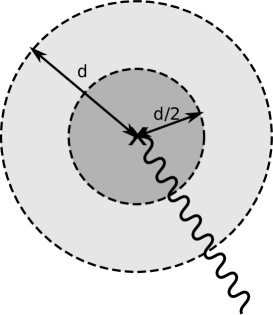
Figure 5: A zoom-in on a small neighborhood of a brane locus. The curvy line denotes the branch-cut around the brane. The concentric circles of radius $d/2$ and $d$ are chosen to be small enough so that they do not intersect any other branch cuts.

Now let us find a gauge transformation that can be used to gauge away vector degrees of freedom living on a particular brane $B_{i_{0}}$. Let us assume a given seven-brane is a Dirichlet brane — i.e., a $(1,0)$ brane — and consider the gauge transformations of the form

$$\Gamma^{I}=\phi^{I}(z,\bar{z})\Lambda(x^{\mu})$$ (41)

where $\phi^{I}$ is a doublet scalar dependent on the internal coordinates while $\Lambda$ is an eight-dimensional one-form. Taking the local holomorphic coordinate around the brane locus $w=0$ to be $w$, one can find some $d$ such that the open neighborhood $|w|<d$ of the brane does not include any other branch cut. Then one can find a real “bump function” $f(w)$ that satisfies the following conditions:

1. $0\leq f(w)\leq 1$ for all $w$, while $f(0)=1$.

2. $f(w)>0$ for $|w|<d/2$.

3. $f(w)=0$ for $|w|>3d/4$.

4. $f(w)$ is $C^{\infty}$ for $|w|<d$ and hence so on the full manifold.

Then, for

$$\begin{pmatrix}\Gamma^{1}\\ \Gamma^{2}\end{pmatrix}=\begin{pmatrix}\phi^{1}\\ \phi^{2}\end{pmatrix}\Lambda=\begin{pmatrix}f(w)\\ 0\end{pmatrix}\Lambda\,,$$ (42)

the gauge transformation (41) is well-defined on the full base manifold. In particular, the value (38) is well defined at each brane locus unambiguously. In fact, for each brane $B_{i}$,

$$A_{\mu}^{i}\rightarrow\begin{cases}A_{\mu}^{i}&\text{when }i\neq i_{0}\\ A_{\mu}^{i}-\Lambda_{\mu}&\text{when }i=i_{0}\end{cases}\,.$$ (43)

The vector field $A^{i_{0}}$ is thereby eaten by the two-form doublet by this CS gauge transformation by setting $\Lambda_{\mu}=A^{i_{0}}_{\mu}$. Likewise, for each brane $B_{i}$ of charge $(p_{i},q_{i})$, we can construct a gauge transformation

$$\begin{pmatrix}\Gamma^{1}\\ \Gamma^{2}\end{pmatrix}={f_{i}\over p_{i}^{2}+q_{i}^{2}}\begin{pmatrix}p_{i}\\ q_{i}\end{pmatrix}\Lambda\,,$$ (44)

with an appropriate bump function $f_{i}$ to absorb $A^{i}$.

Hence, in “unitary gauge” where all the gauge fields living on the world-volume of the seven-branes are eaten, the term (36) of the Lagrangian becomes

$$-{\mu_{8}\over 4}\sum_{i=1}^{24}\int d^{8}x\sqrt{-g}(p_{i}B_{\mu\nu}+q_{i}C_{\mu\nu})^{2}\,.$$ (45)

Regardless of this term, which looks like an eight-dimensional mass term for the tensor fields, we still find modes of the tensor fields responsible for massless degrees of freedom of the 8D effective theory. These come from modes with components transverse to the seven-branes. We proceed to examine these modes in the next section.

4 $SL(2,{\mathbb{{Z}}})$ Doublet Harmonic One-forms

In this section, we show how 20 massless vector fields arise in F-theory compactifications on K3 from the type IIB perspective. In section 4.1, we define what we mean by $SL(2,{\mathbb{{Z}}})$ doublet harmonic one-forms and show that the doublet two-form of type IIB theory can be reduced along these one-forms to yield massless vectors in the eight-dimensional theory. In the following two sections, we study these zero modes from two different points of view. In section 4.2, we show that these harmonic forms represent elements of the first cohomology group of a certain sheaf living on the base manifold $\bar{S}$. We also derive that the dimension of this cohomology group is 20. In section 4.3, we establish the correspondence between doublet harmonic one-forms and certain closed two-forms — namely, the “semi-flat harmonic two-forms” — living inside the underlying K3 manifold $\bar{M}$. We end by showing how other particles and fields of the 8D theory couple to the vectors obtained by reducing along these one-forms in section 4.4. The various couplings are shown to encode the geometric data of $\bar{M}$.

4.1 Definition

In this section, we show how massless vectors arise in F-theory compactifications on K3. These are obtained upon KK-reduction of the $SL(2,{\mathbb{{Z}}})$ doublet two-forms of the type IIB theory along doublet one-form zero modes. In particular, we derive the “zero mode condition” or the “harmonicity condition” (7) a $SL(2,{\mathbb{{Z}}})$ doublet one-form $\xi^{I}$ living in the compactification manifold $S$ must satisfy.

Let us consider the KK-reduction of the doublet two-form fields in the F-theory background along some doublet zero-mode. The KK-reduction ansatz is given as

$$B^{I}=\phi^{I}(z,{\bar{z}})\wedge b$$ (46)

where $\phi$ is some doublet $k$-form aligned along the internal direction and $b$ is an eight-dimensional $(2-k)$-form field. In order for $b$ to be massless, $\phi$ must be closed:

$$d\phi^{I}=0\,.$$ (47)

At the same time, $\phi^{I}$ must respect the monodromies defined by the background, i.e., it must exhibit the same $SL(2,{\mathbb{{Z}}})$ transformations that the field strengths experience as they cross the branch cuts. In particular, upon counter-clockwise rotation around a brane locus $B_{i}$, $\phi^{I}$ must transform as

$$\begin{pmatrix}\phi^{1}\\ \phi^{2}\end{pmatrix}\rightarrow\begin{pmatrix}1-p_{i}q_{i}&-q_{i}^{2}\\ p_{i}^{2}&1+p_{i}q_{i}\end{pmatrix}\begin{pmatrix}\phi^{1}\\ \phi^{2}\end{pmatrix}\equiv M_{i}\begin{pmatrix}\phi^{1}\\ \phi^{2}\end{pmatrix}\,.$$ (48)

There are two ways of seeing why such behavior should be imposed on $\phi^{I}$. The first way is by examining the field strength of the doublet two-form — as explained in the previous section, in order for the action of the type IIB theory to be invariant under moving branch cuts, the field strength-doublet $(dB,dC)$ must exhibit the monodromies (39). The constraint on $\phi^{I}$ follows by applying this condition to the ansatz (46). Another way of seeing this constraint is to consider the normalization of the mode $\phi^{I}$, which is given by

$$\int_{\tilde{S}}\mathcal{M}_{IJ}\phi^{I}\wedge*\phi^{J}\,.$$ (49)

Unless $\phi^{I}$ exhibits the correct monodromies, the normalization (49) is not well defined — in fact, it would vary as one moves the branch cuts around. On the other hand, when $\phi^{I}$ exhibit the desired monodromies, we can define the norm

$$\int_{\bar{S}}\mathcal{M}_{IJ}\phi^{I}\wedge*\phi^{J}\equiv\int_{\tilde{S}}\mathcal{M}_{IJ}\phi^{I}\wedge*\phi^{J}\,.$$ (50)

It was pointed out in Vafa:1996xn that there is no way of turning on the two-form fields along the internal directions and also satisfying the required monodromies. Also, it is clear that there does not exist any non-zero closed zero-forms — i.e., constant scalars — that exhibit monodromic behavior. The interesting closed forms that yield massless particles in eight-dimensions are the one-forms, which we denote by

$$\xi^{k}=\begin{pmatrix}\xi^{k,1}\\ \xi^{k,2}\end{pmatrix}\,.$$ (51)

Hence we wish to find closed doublet one-forms living in the base manifold $\bar{S}$.

These one-forms must be normalizable with respect to the Hermitian inner-product

$$\langle\xi^{k},\xi^{l}\rangle\equiv\int_{\tilde{S}}\mathcal{M}_{IJ}\xi^{k,I}\wedge*\xi^{l,J}$$ (52)

defined by the Lagrangian, i.e.,

$$\langle\xi^{k},\xi^{k}\rangle<\infty\,.$$ (53)

Note that since $\xi^{k}$ have monodromies around the brane loci, their components exhibit logarithmic behavior at these points. Despite such singular behavior, the modes can nevertheless be normalizable. For example, when the singularities of $\xi^{k}$ are logarithmic, the integral near the brane loci

$$\propto\int_{0}^{\epsilon}drr(\ln r)^{k}$$ (54)

is convergent.

As with KK-reduction of any $p$-form, the closed one-forms $\xi^{k}$ we reduce along are defined up to an exact form $d\varphi$, where $\varphi$ is a doublet of zero-forms. This freedom comes as a remnant of the “CS gauge symmetry” of the type IIB background. Such an ambiguity is fixed by demanding that $\xi^{k}$ is harmonic with respect to the Hermitian inner-product defined by the Lagrangian, i.e.,

$$d*\mathcal{M}_{IJ}\xi^{k,J}=0\,.$$ (55)

A simple computation shows that imposing this condition assures that $\xi^{k}$ has minimum norm given the “cohomology class” of $\xi^{k}$ is fixed. In other words,

$$\langle\xi^{k},\xi^{k}\rangle<\langle\xi^{k},\xi^{k}\rangle+\langle d\varphi,d\varphi\rangle=\langle\xi^{k}+d\varphi,\xi^{k}+d\varphi\rangle$$ (56)

for any non-trivial CS gauge transformation $d\varphi\neq 0$ when $\xi^{k}$ satisfies (55). Hence, the condition (55) singles out elements of a certain cohomology class, just as the usual harmonicity condition singles out a harmonic form in a given de Rham cohomology class. We describe this cohomology in more detail in the following section.

A source of worry for equation (56) is that integration by parts has been used in obtaining the equality — for the most general CS gauge transformation $\varphi$, the cross terms in the integral of interest may have boundary terms. Such boundary terms arise in the case that $\varphi$ exhibit monodromic behavior that is affine rather than linear. To be more precise, let us first examine how $\varphi$ is allowed to behave as we rotate around a brane locus. In order for the $\xi^{k}+d\varphi$ to have a well defined norm, $d\varphi$ must exhibit the monodromy

$$\begin{pmatrix}d\varphi^{1}\\ d\varphi^{2}\end{pmatrix}\rightarrow\begin{pmatrix}1-p_{i}q_{i}&-q_{i}^{2}\\ p_{i}^{2}&1+p_{i}q_{i}\end{pmatrix}\begin{pmatrix}d\varphi^{1}\\ d\varphi^{2}\end{pmatrix}$$ (57)

around brane $B_{i}$. $\varphi$ itself, however, does not have to display this monodromy — in fact, it is allowed to shift:

$$\begin{pmatrix}\varphi^{1}\\ \varphi^{2}\end{pmatrix}\rightarrow\begin{pmatrix}1-p_{i}q_{i}&-q_{i}^{2}\\ p_{i}^{2}&1+p_{i}q_{i}\end{pmatrix}\begin{pmatrix}\varphi^{1}\\ \varphi^{2}\end{pmatrix}+C_{i}\begin{pmatrix}-q_{i}\\ p_{i}\end{pmatrix}\,.$$ (58)

Note that the shift must be in the direction $(-q_{i},p_{i})^{t}$, as the values $p_{i}\varphi^{1}+q_{i}\varphi^{2}$ must be well-defined at the brane locus. In the event that $C_{i}\neq 0$, the integration by parts we have used in (56) is no longer valid, as there would exist boundary terms living on $\partial\tilde{S}$ — a contour encircling the “cuts” we have used to define a type IIB frame — that do not cancel out.

What makes the equality of (56) work is that we only allow gauge transformations such that

$$p_{i}\varphi^{1}(z_{i},\bar{z}_{i})+q_{i}\varphi^{2}(z_{i},\bar{z}_{i})=0$$ (59)

at seven-brane loci $(z_{i},\bar{z}_{i})$. This is because we are computing the eight-dimensional massless spectrum in a “unitary gauge” where all the seven-brane world-volume vector fields are eaten by tensor degrees of freedom. The condition (59) ensures that the fluctuations we consider still satisfy the unitary gauge condition. In appendix A, we show that $C_{i}=0$ for gauge transformations $\varphi$ that do not excite seven-brane vector fields and keep the mode $\xi^{k}+d\varphi$ normalizable.

Let us conclude this section by summarizing the definition of a $SL(2,{\mathbb{{Z}}})$ doublet harmonic one-form $\xi$:

1. $$\xi \begin{pmatrix}\xi^{1}\\ \xi^{2}\end{pmatrix}\rightarrow\begin{pmatrix}1-p_{i}q_{i}&-q_{i}^{2}\\ p_{i}^{2}&1+p_{i}q_{i}\end{pmatrix}\begin{pmatrix}\xi^{1}\\ \xi^{2}\end{pmatrix} B_{i} d\xi^{I}=0\,,\quad d*\mathcal{M}_{IJ}\xi^{J}=0\,. \langle\xi,\eta\rangle\equiv\int_{\tilde{S}}\mathcal{M}_{IJ}\xi^{I}\wedge*\eta^{J}\,.$$ is doublet of one-forms exhibiting the monodromy (48); around brane locus . 2. It must satisfy the defining equations (7): 3. It must be normalizable with respect to the inner-product (52):

In the subsequent sections, we go on to count and construct such harmonic one-forms.

4.2 Coordinate-free Description of Doublet One-forms

In this section, we give a coordinate-free description of $SL(2,\mathbb{Z})$ doublet one-forms on $S$ in terms of certain sheaves. We also show that the dimension of the space of doublet harmonic one-forms is equal to $20$, by applying results by Zucker Zucker about polarized variations of Hodge structure on curves.

Recall that $\bar{f}\colon\bar{M}\to\bar{S}$ is an elliptically fibered K3-surface with a section; here $\bar{S}$ is the complex projective line. We assume that there are exactly $24$ singular fibers, each with a single ordinary double point — for degree reasons, the section cannot pass through any of the $24$ special points. If we denote by $S\subseteq\bar{S}$ the complement of the $24$ singular values, and by $M=\bar{f}^{-1}(S)$ the open surface obtained by removing the singular fibers from $\bar{M}$, then the restriction $f\colon M\to S$ is a smooth family of elliptic curves.

Sheaf theory allows us to make some of the constructions coordinate free. Instead of choosing $A$-cycles and $B$-cycles over a dense open subset $\tilde{S}$ of $S$, we can directly obtain the corresponding fiber bundle with fiber $\mathbb{Z}^{2}$ by defining

$$\mathcal{H}_{\mathbb{Z}}=R^{1}f_{\ast}\mathbb{Z}$$

as the first higher direct image sheaf of the constant sheaf $\mathbb{Z}$ on $M$. At each point $s\in S$, the stalk of the sheaf $\mathcal{H}_{\mathbb{Z}}$ is equal to the first cohomology group $H^{1}(E_{s},\mathbb{Z})$ of the corresponding elliptic curve $E_{s}=f^{-1}(s)$. Making a choice of $A$-cycle and $B$-cycle over a simply-connected open subset of $S$ is the same thing as choosing a local trivialization of the sheaf $\mathcal{H}_{\mathbb{Z}}$.

Now the first cohomology group $H^{1}(E,\mathbb{Z})$ carries a polarized Hodge structure of weight $1$. The Hodge structure is given by the decomposition

$$H^{1}(E,\mathbb{C})\simeq H^{1}(E,\mathbb{Z})\otimes_{\mathbb{Z}}\mathbb{C}=H^{1,0}(E)\oplus H^{0,1}(E)$$

according to type; the polarization is given by the intersection form

$$Q(\alpha,\beta)=\int_{E}\alpha\wedge\beta.$$

It is a polarization because of the Riemann bilinear relations: the Hermitian form $\alpha\mapsto i^{p-q}Q(\alpha,\overline{\alpha})$ is positive-definite on the subspace $H^{p,q}(E)$, and the above decomposition is orthogonal with respect to the resulting Hermitian inner product on $H^{1}(E,\mathbb{C})$.

Because the same is true at every point of $S$, the locally constant sheaf $\mathcal{H}_{\mathbb{Z}}$ is part of a polarized variation of Hodge structure $\mathcal{H}$ on $S$. Let us briefly explain what this means. The holomorphic vector bundle $\mathcal{H}=\mathcal{H}_{\mathbb{Z}}\otimes_{\mathbb{Z}}\mathscr{O}_{S}$ has a natural flat connection

$$\nabla\colon\mathcal{H}\to\Omega_{S}^{1}\otimes_{\mathscr{O}_{S}}\mathcal{H},$$

with the property that the sheaf of flat sections is isomorphic to $\mathcal{H}_{\mathbb{C}}$. Both $\mathcal{H}$ and $\nabla$ can also be constructed geometrically, and are known as a Gauss-Manin system. The additional data coming from the polarized Hodge structures on the cohomology of the fibers are a holomorphic subbundle $F^{1}\mathcal{H}$, corresponding to the subspace $H^{1,0}(E_{s})$ in the above decomposition, and a flat pairing $\mathcal{H}_{\mathbb{Z}}\otimes_{\mathbb{Z}}\mathcal{H}_{\mathbb{Z}}\to\mathbb{Z}$, corresponding to the intersection pairing.

Because the locally constant sheaf $\mathcal{H}_{\mathbb{Z}}$ contains the information about the monodromy of $A$-cycles and $B$-cycles, and because $\mathcal{H}=\mathcal{H}_{\mathbb{Z}}\otimes_{\mathbb{Z}}\mathscr{O}_{S}$, an $SL(2,\mathbb{Z})$ doublet $k$-form is easily seen to be the same thing as a smooth $k$-form on $S$ with coefficients in the vector bundle $\mathcal{H}$. We denote the space of all such forms by the symbol

$$A^{k}(S,\mathcal{H}).$$

The connection $\nabla$ can be extended to an operator from doublet $k$-forms to doublet $(k+1)$-forms, and the resulting complex

computes the cohomology groups $H^{k}(S,\mathcal{H}_{\mathbb{C}})$ of the locally constant sheaf $\mathcal{H}_{\mathbb{C}}$, by a version of the Poincaré lemma.

One might expect naively that the number of zero-modes defined in the previous section can be obtained by computing the dimension of the cohomology group $H^{1}(S,\mathcal{H}_{\mathbb{Q}})$. This is not true, since elements of this cohomology group can exhibit singular behavior near the discriminant locus, and may therefore not be normalizable with respect to the inner-product defined in the previous section. In fact, the dimension can be shown to be $20+24=44$. Instead, the correct cohomology group to consider is

$$H^{1}\bigl{(}\bar{S},j_{\ast}\mathcal{H}_{\mathbb{Q}}\bigr{)},$$

where $j\colon S\hookrightarrow\bar{S}$ denotes the inclusion map of $S$ into $\bar{S}$. In appendix B, we use some theorems by Zucker Zucker to prove that $H^{k}\bigl{(}\bar{S},j_{\ast}\mathcal{H}_{\mathbb{Q}}\bigr{)}=0$ for $k\neq 1$, and that

$$\dim H^{1}\bigl{(}\bar{S},j_{\ast}\mathcal{H}_{\mathbb{Q}}\bigr{)}=20,$$

as expected. Moreover, it is shown in Zucker that the first cohomology group is isomorphic to the subspace of $A^{1}(S,\mathcal{H})$ consisting of forms that are square-integrable and harmonic (with respect to the Hodge metric on $\mathcal{H}$ and the Poincaré metric on $S$). These two conditions are exactly the same as in the previous section, and so we deduce that the space of $SL(2,\mathbb{Z})$ doublet harmonic one-forms is indeed $20$-dimensional.

The work of Zucker also endows $H^{1}\bigl{(}\bar{S},j_{\ast}\mathcal{H}_{\mathbb{Q}}\bigr{)}$ with a polarized Hodge structure of weight $2$. This Hodge structure is compatible with that on $H^{2}(\bar{M},\mathbb{Q})$; more precisely, there is a natural morphism

$$H^{2}(\bar{M},\mathbb{Q})_{\perp}\to H^{1}\bigl{(}\bar{S},j_{\ast}\mathcal{H}_{\mathbb{Q}}\bigr{)},$$

and this morphism is an isomorphism of polarized Hodge structures. We will see below how this statement about cohomology groups can be sharpened to a result about spaces of harmonic forms.

4.3 Construction from Harmonic Two-forms on ${M}$

In this section, we explain how to construct the doublet harmonic one-forms from the point of view of the K3 manifold $\bar{M}$. To be more precise, we show that there is a correspondence between the doublet harmonic one-forms and two-forms of the K3 manifold that are harmonic with respect to the semi-flat metric Greene:1989ya . We conjecture that these “semi-flat harmonic two-forms” can be obtained as a limit of harmonic two-forms of the K3 manifold with respect to the Calabi-Yau metric.

Let us begin by noting that a natural way to obtain a doublet of closed one-forms on the base manifold $S$ of the elliptic fibration, that displays the monodromies of the cycles of the fiber, is by using two-forms of the underlying K3 geometry. Consider a smooth closed two-form $\Xi$ living inside the $M$ obtained by excising the 24 singular fibers of the K3 manifold $\bar{M}$. Now for each point $z$ on the base manifold, let us define a doublet of forms

$$\xi=\begin{pmatrix}\int_{\alpha}\Xi\\ \int_{\beta}\Xi\end{pmatrix}$$ (60)

where the integration cycles are taken to lie within the holomorphic fiber above the point $z$. $\alpha$ and $\beta$ are the $A$ and $B$-cycle of the fibration used to define the type IIB frame. If $\xi$ is “well defined,” it is a doublet of one-forms that exhibit the correct monodromies. It is also closed due to the closedness of $\Xi$.

In order for $\xi$ to be well defined, the projection of $\Xi$ to each fiber must vanish. Meanwhile, components of $\Xi$ with both legs parallel to the base would not affect $\xi$ and should be “gauged away” if one wishes to establish a one-to-one correspondence between one-forms on the base and two-forms in the full manifold. Let us hence assume the components of $\Xi$ with both legs along either the fiber or the base direction vanish. A better presentation of this condition is given shortly.

For $\xi$ to be harmonic as defined in (7), an additional condition on $\Xi$ must be imposed. It is in fact that $\Xi$ should be harmonic with respect to the semi-flat metric constructed in Greene:1989ya . More precisely, we consider the family of semi-flat metrics whose Kähler form $J_{t}$ is given by

$$J_{t}/i={W(z,\bar{z})\over t}{\theta}^{z}\wedge{{\theta}^{\bar{z}}}+{t\over W(z,\bar{z})}{\theta}^{w}\wedge{\theta}^{\bar{w}}$$ (61)

for some function $W$ GrossWilson . The one forms ${\theta}^{z}$ and ${\theta}^{\bar{z}}$ are defined to as

$${\theta}^{z}=dz,\quad{\theta}^{\bar{z}}=d\bar{z}\,,$$ (62)

where $z$ is the holomorphic coordinate on the base. ${\theta}^{w}$ and ${\theta}^{\bar{w}}$, which we define shortly after, are one-forms aligned along the fiber direction.

The semi-flat metric is a Ricci-flat Kähler metric on the K3 manifold, which is locally defined by the hypersurface equation

$$y^{2}=x^{3}+f_{8}(z)x+g_{12}(z)\,.$$ (63)

$W$ is given by (23) — we can in fact use the Thomae formula to obtain the expression

$$W(z,\bar{z})={4\pi^{2}\over 2^{1/6}}{\tau_{2}|\eta(\tau)|^{4}\over|\Delta|^{1/6}}=-i\int{\bar{\lambda}}\wedge{\lambda}\,.$$ (64)

${\lambda}=dx/y$ here is the unique holomorphic one-form of the fiber while the integral is taken to be along the elliptic fiber at $z$. This relation is derived in appendix C — the normalization constant is added for aesthetic reasons. The one-form ${\theta}^{w}$ can be expressed using the canonical holomorphic coordinate

$$\zeta(x)=\int^{x}{\lambda}$$ (65)

— where the starting point of the integral is the locus of the zero section on the fiber — by

$${\theta}^{w}=d\zeta-{(\partial{\lambda},{\bar{\lambda}})\zeta-(\partial{\lambda},{\lambda})\bar{\zeta}\over({\lambda},{\bar{\lambda}})}dz\,.$$ (66)

The one-form $\partial{\lambda}$ living on the fiber can be explicitly written as

$$\partial{\lambda}=-{f_{8}^{\prime}(z)x+g_{12}^{\prime}(z)\over 2y^{3}}dx.$$ (67)

While $\partial{\lambda}$ shows singular behavior at certain points on the elliptic curve, it is a “differential of the third kind,” i.e., its integral over closed cycles of the elliptic curve are nevertheless well-defined. Hence the values $(\partial{\lambda},{\bar{\lambda}})$ and $(\partial{\lambda},{\lambda})$ are well-defined for the inner-product

$$(\kappa,{\lambda})\equiv\int_{\alpha}\kappa\int_{\beta}{\lambda}-\int_{\beta}\kappa\int_{\alpha}{\lambda}\,.$$ (68)

The one form ${\theta}^{w}$ may at first sight look rather peculiar — it, however, can be re-written in a simple way, using the coordinates $x_{1}$ and $x_{2}$ which parametrize the flat elliptic fiber such that

$$x_{1}\cong x_{1}+1,\quad x_{1}+ix_{2}\cong x_{1}+ix_{2}+\tau(z)\,.$$ (69)

Upon acknowledging that

$$(\int_{\alpha}{\lambda})x_{1}+(\int_{\beta}{\lambda})x_{2}=\zeta\,,$$ (70)

it can be shown that

$${1\over W(z,\bar{z})}{\theta}^{w}\wedge{\theta}^{\bar{w}}={1\over 2\tau_{2}}(dx_{1}+\tau dx_{2})\wedge(dx_{1}+\bar{\tau}dx_{2})\,.$$ (71)

We hence see that $J_{t}$ is aligned in the base and fiber directions — it is orthogonal to cycles of the manifold that are orthogonal to the class of the fiber and the base. Despite the nice properties of the semi-flat metric, it fails to be a smooth Calabi-Yau metric, as it degenerates at the discriminant locus of the elliptic fibration. It has, however, been shown that it is a good approximation to the Calabi-Yau metric on the K3 manifold with fiber size $t$ as $t$ approaches zero GrossWilson . It also is a smooth, non-degenerate Calabi-Yau metric of the open manifold $M$.

In order for a doublet one-form $\xi$ constructed from a two-form $\Xi$ living inside this manifold to be well defined, $\Xi_{z\bar{z}}=\Xi_{w\bar{w}}=0$, as discussed at the beginning of this section. This condition can be expressed using the following harmonic two-forms with respect to $J_{t}$:

$$B\equiv{W(z,\bar{z})}{\theta}^{z}\wedge{{\theta}^{\bar{z}}},\quad F\equiv{1\over W(z,\bar{z})}{\theta}^{w}\wedge{\theta}^{\bar{w}}\,,$$ (72)

as

$$\Xi\wedge B=\Xi\wedge F=0\,.$$ (73)

Although $B$ and $F$ behave singularly at discriminant loci, they nevertheless represent cohomology classes of the manifold $\bar{M}$. While de Rham cohomology is defined by using smooth differential forms, a form $\Xi$ that is not necessarily smooth still represents a cohomology class as long as its integrals along homology classes are well-defined. In this case, the cohomology class of $\Xi$ can is given by the dual cohomology class of

$$(\int_{C_{i}}\Xi)[C_{i}]\,,$$ (74)

with respect to the canonical pairing

$$\langle C,\omega\rangle=\int_{C}\omega$$ (75)

between forms and cycles. Here $C_{i}$ is the basis of the homology group of the manifold. The forms $B$ and $F$ are in fact dual to the base and the fiber class of $\bar{M}$. In particular, it can be shown that

$$\int_{\text{Base}}B=\int_{\bar{M}}{\Omega}\wedge\bar{\Omega},\quad\int_{\text{Fiber}}F=1\,,\quad\int_{\text{Base}}F=\int_{\text{Fiber}}B=0\,,$$ (76)

while the integrals of $B$ and $F$ over cycles orthogonal to the base and fiber vanish. It is worth noting that the forms $B$ and $F$ are normalizable with respect to the semi-flat metric at finite $t$;

$${1\over t^{2}}\int_{\bar{M}}B\wedge*_{sf}B={t^{2}}\int_{\bar{M}}F\wedge*_{sf}F=\int_{\bar{M}}{\Omega}\wedge\bar{\Omega}\,.$$ (77)

Here, $*_{sf}$ denotes the Hodge dual with respect to the semi-flat metric while ${\Omega}$ is the holomorphic two-form.

In appendix D, we show that when $\Xi$ is harmonic with respect to the semi-flat metric, and its components $\Xi_{z\bar{z}}$ and $\Xi_{w\bar{w}}$ vanish,

$$*\mathcal{M}_{IJ}\xi^{J}=\begin{pmatrix}\int_{\beta}*_{sf}\Xi\\ -\int_{\alpha}*_{sf}\Xi\end{pmatrix}$$ (78)

for $\xi$ constructed by (60). In this case, the condition

$$d*\mathcal{M}_{IJ}\xi^{J}=0$$ (79)

is satisfied since $*_{sf}\Xi$ is also closed. Given this result, it is straightforward to obtain the inner-product (52) of harmonic one-form doublets $\xi$ and $\eta$ constructed from harmonic two-forms $\Xi$ and $H$ as an integral on $M$. It is a simple exercise to show in fact that

$$\begin{split}\langle\xi,\eta\rangle&\equiv\int_{S}\mathcal{M}_{IJ}\xi^{I}\wedge*\eta^{J}=\int_{S}(\int_{\alpha}\Xi{\int_{\beta}}*_{sf}H-{\int_{\alpha}}*_{sf}H{\int_{\beta}}\Xi)\\ &=\int_{M}\Xi\wedge*_{sf}H\equiv\int_{\bar{M}}\Xi\wedge*_{sf}H\,,\end{split}$$ (80)

using properties of harmonic forms of the semi-flat metric derived in appendix D. Hence in order for $\xi$ to be normalizable as defined in section 4.3, $\Xi$ must also be normalizable with respect to the canonical inner-product defined by the semi-flat metric.

Before we carry further on, let us sum up the properties of the two-forms $\Xi$ that produce doublet harmonic one-forms upon integrating along cycles of the fiber:

1. $$\Xi \Xi *_{sf}\Xi \Xi \Xi\wedge B=\Xi\wedge F=0\,, B F \Xi \langle\Xi,H\rangle\equiv\int_{\bar{M}}\Xi\wedge*_{sf}H\,.$$ is harmonic with respect to the semi-flat metric, i.e., both and are closed. 2. satisfies (81) for the two-forms and defined in equation (72). 3. is normalizable with respect to the inner-product (82)

Let us denote such harmonic two-forms, “semi-flat harmonic two-forms.” It is worth commenting that the definition of semi-flat harmonic forms is independent of the parameter $t$. This is because the Hodge dual $*_{sf}$ acting on a two-form $\Xi$ is independent of $t$ when $\Xi$ satisfies (81). This, in particular, implies that these harmonic forms can be defined at the singular point $t=0$.

So far, we have shown that there is a map from semi-flat harmonic two-forms of a dense open subset $M$ of the K3 manifold $\bar{M}$ to doublet harmonic one-forms on the base $\bar{S}$. We show that this map is actually bijective in appendix D. This implies that the 20-dimensional space of doublet one-forms $H^{1}(\bar{S},j_{*}\mathcal{H}_{\mathbb{R}})$ can be lifted to a 20-dimensional space of semi-flat harmonic two-forms. These two-forms are a priori defined only on $M$.

A natural question to ask is whether these 20 semi-flat harmonic two-forms are related to cohomology classes of the K3 manifold $H^{2}(\bar{M})$. In appendix E we show that this is in fact the case. To be more precise, let us first describe the cohomology group of the open manifold $M$. The dual homology group of $M$ is generated by 21 elements inherited from $\bar{M}$ — the class of the section becomes trivial in $M$ — and 24 cycles attached to each degenerate fiber. The 24 cycles are represented by tori $T_{i}$ constructed by rotating an invariant cycle around a degeneration locus $B_{i}$. In proposition 160, we prove that the 20 semi-flat harmonic two-forms $\{\Xi_{k}\}$ span the subgroup of $H^{2}(M)$ obtained from pulling back $H^{2}(\bar{M})_{\perp}$ via the inclusion map $M\hookrightarrow\bar{M}$. A more practical way to say this is that $\{\Xi_{k}\}$ can be extended to the manifold $\bar{M}$, and that it represents a basis of the cohomology group $H^{2}(\bar{M})_{\perp}$. Recall that $H^{2}(\bar{M})_{\perp}$ is defined to be the orthogonal space to the cohomology classes $[B]$ and $[F]$, by which we denote the duals of the homology classes of the base and fiber, respectively.

Let us provide an intuitive sketch of why the dual homology elements of $\{\Xi_{k}\}$ must lie within the image of $H_{2}(\bar{M})_{\perp}$ in $H_{2}(M)$. This turns out to be a consequence of imposing normalizability on $\Xi_{k}$. We note that since the semi-flat harmonic two-forms are orthogonal to the base and fiber directions, it is enough to show that $\{\Xi_{k}\}$ are orthogonal to the cycles $T_{i}$ described in the preceding paragraph. To show this, let us assume that a semi-flat harmonic two-form $\Xi$ has a non-trivial integral over some cycle $T_{i}$, i.e.,

$$\int_{T_{i}}\Xi=C_{i}\,.$$ (83)

Recall that $T_{i}$ is constructed by rotating the invariant cycle $(p_{i}\alpha+q_{i}\beta)$ around the degeneration locus $B_{i}$. Denoting the doublet harmonic one-form constructed from $\Xi$ as $\xi$, this implies that

$$\oint_{c}(p_{i}\xi^{1}+q_{i}\xi^{2})=C_{i}$$ (84)

for a contour $c$ surrounding $B_{i}$. Following the latter part of appendix A, it can then be shown that such $\xi$ cannot be normalizable with respect to the norm defined for doublet one-forms, due to the divergent behavior of $\xi$ near $B_{i}$. It follows that $\Xi$ is not normalizable with respect to the semi-flat metric, hence concluding the proof.

The fact that the semi-flat harmonic two-forms form a basis for $H^{2}(\bar{M})_{\perp}$ suggests that they can be related to harmonic forms of the K3 manifold with respect to a class of smooth Calabi-Yau metrics in the following way. Let us consider a class of smooth, non-degenerate Ricci flat metrics with Kähler form $K_{t}$ that satisfies the following conditions:

1. The dual homology class of $K_{t}$ is aligned in the direction of the class of the base and the fiber.

2. $K_{t}\wedge K_{t}=2{\Omega}\wedge\bar{\Omega}$ for the holomorphic two-form ${\Omega}$ of the K3 manifold. In terms of the one-form $\lambda$ we have been using, this condition can be re-expressed as

   $$K_{t}\wedge K_{t}=2{\Omega}\wedge\bar{\Omega}=2{\lambda\wedge dz}\wedge{\bar{\lambda}\wedge d\bar{z}}\,.$$ (85)

3. $\int_{\bar{f}^{-1}(z)}K_{t}=t$ for any point $z$ in the base, i.e., the fiber size with respect to this metric is given by $t$. Recall that $\bar{f}$ is the projection map of the fibration.

The semi-flat metric is also a Ricci flat metric whose Kähler form $J_{t}$ satisfies these conditions. While $J_{t}$ is degenerate at the discriminant locus, $J_{t}$ and $K_{t}$ are closely related — in fact, $tJ_{t}$ and $tK_{t}$ have been shown to coincide in the limit $t\rightarrow 0$ GrossWilson . Since $J_{t}$ approximates $K_{t}$ well in the small-$t$ limit, we can expect that there is a one-to-one correspondence between the semi-flat harmonic two forms and harmonic two-forms of the Calabi-Yau metric in the subspace $H^{2}(\bar{M})_{\perp}$. More precisely, we can put forth the following

Proposal : For the stated class of Calabi-Yau metrics $K_{t}$, let $\{\omega_{1},\cdots,\omega_{20}\}$ denote the linearly independent harmonic forms spanning the 20-dimensional subspace $H^{2}(\bar{M})_{\perp}$ of the cohomology group spanned by elements orthogonal to the classes $[B]$ and $[F]$. In the limit $t\rightarrow 0$, these 20 harmonic forms stay linearly independent and form a basis $\{\Xi_{1},\cdots,\Xi_{20}\}$ of the semi-flat harmonic two-forms.

Given that the forms $\{\omega_{1},\cdots,\omega_{20}\}$ do not develop singularities that obstruct the normalizability condition, it can be shown that $\omega_{k}$ stay linearly independent. This is done by examining the duals of the cohomology classes of $\omega_{k}$. Since the duals of $\{\omega_{k}\}$ are linearly independent in the homology group, $\{\omega_{k}\}$ also remain linearly independent as two-forms.

A crucial test for the validity of the proposal would be to verify that the limits of $\omega_{k}$ satisfy the orthogonality condition (81). This is because orthogonality at the level of cohomology does not guarantee orthogonality at the level of forms. Let us consider harmonic two-forms $\omega_{k}$ with respect to the Calabi-Yau metric whose cohomology class are orthogonal to $[B]$ and $[F]$, i.e.,

$$\int_{\bar{M}}\omega_{k}\wedge{\cal B}_{t}=\int_{\bar{M}}\omega_{k}\wedge{\cal F}_{t}=0\,,$$ (86)

where ${\cal B}_{t}$ and ${\cal F}_{t}$ are harmonic forms in the cohomology classes $[B]$ and $[F]$. We have added the subscripts to emphasize that while the cohomology classes are defined irrespective of the metric, the harmonic forms have a metric dependence. While the conditions (86) do not imply that the two integrands vanish at every point, they imply “half” of these two conditions. Since the Kähler form $K_{t}$ of the metric — which is harmonic — is given by a linear combination of ${\cal B}_{t}$ and ${\cal F}_{t}$ by assumption, and since the Lefschetz action commutes with the Laplacian operator, it follows that

$$\omega_{k}\wedge K_{t}=0\,.$$ (87)

It would be interesting to verify that the other half of the constraint is satisfied as the fiber size is taken to zero.

A natural way to map the semi-flat harmonic forms $\{\Xi_{k}\}$ to the corresponding harmonic forms $\{\omega_{k}\}$ at finite $t$ is provided by M-theory/F-theory duality Vafa:1996xn . Let us consider the eight-dimensional theory obtained by compactifying F-theory on K3 manifold $\bar{M}$, and let $a_{k}$ be the massless vector fields obtained by KK-reducing the doublet two-form fields of type IIB along one-forms $\xi^{k}$ constructed from $\Xi_{k}$. The seven-dimensional effective theory obtained upon further compactification on a $S^{1}$ of radius $\sim\alpha^{\prime}/t^{-1/2}$ — where $\alpha^{\prime}$ is the Regge slope of the type II string — is dual to M-theory compactified on $\bar{M}$ with Calabi-Yau metric $K_{t}$. The seven-dimensional vector fields $\tilde{a}_{k}^{\prime}$ — which are modes of $a_{k}$ constant along the $S^{1}$ — are obtained by KK-reducing the M-theory three-form along harmonic forms $\omega_{k}$. The inverse coupling of the vector fields of the 8D theory are given by the inner-products of the semi-flat harmonic forms $\Xi_{k}$ (82). Meanwhile, upon reduction on a circle, the corresponding 7D couplings receive quantum corrections from charged particles winding around the compactification circle. The quantum corrected inverse couplings can be computed by the inner-product of the harmonic forms $\omega_{k}$ with respect to the Calabi-Yau metric. Hence, in this sense, $\omega_{k}$ can be thought of as a “quantum corrected” version of $\Xi_{k}$.

In the next subsection, we investigate various properties of the vector fields of the 8D theory whose construction we have been studying up to this point. Let us conclude this section by summarizing what we have learned so far about the massless vector field spectrum of the effective 8D theory of the F-theory compactification on $\bar{M}$, and setting the conventions for the next section:

1. The massless vector spectrum comes from reducing the type IIB doublet two-forms along doublet harmonic one-forms. We denote the massless vectors $a^{k}$ and the one-forms $\xi^{k}$.

2. There are 20 linearly independent $\xi^{k}$.

3. The components of $\xi^{k}$ can be obtained by integrating the “semi-flat harmonic two-forms” $\Xi_{k}$ of $\bar{M}$ along the $A$ and $B$-cycles of the elliptic fiber.

4. $\{\Xi_{1},\cdots,\Xi_{20}\}$ are closed two-forms whose dual two-cycles span $H_{2}(\bar{M})_{\perp}$.

4.4 Properties of KK-reduced Vector Fields

In this section, we explore the properties of the massless vector fields of the 8D theory obtained by KK-reduction. We first compute the charges of string junctions under these vector fields. We go on to relate the vector fields to seven-brane world-volume vector fields through a particular CS gauge transformation. We conclude the section by computing the Chern-Simons couplings of the 8D effective theory involving the massless vector fields.

The massive charged states of the 8D theory come from string junctions stretching inside of the base manifold $\tilde{S}$ and ending on the seven-branes. Any junction with charge vector $\sigma$ can be represented by a tree of directed segments $\{s_{l}\}$ of $n_{l}(p_{l},q_{l})$ strings — where $p_{l}$ and $q_{l}$ are mutually prime — that either begin/end at $(p_{l},q_{l})$ branes or junction points. The segments $\{s_{l_{i}}\}$ meeting at the junction points $P_{i}$ must satisfy the charge conservation condition

$$\sum_{l_{i}\rightarrow P_{i}}n_{l_{i}}(p_{l_{i}},q_{l_{i}})-\sum_{l_{i}\leftarrow P_{i}}n_{l_{i}}(p_{l_{i}},q_{l_{i}})=0\,,$$ (88)

where the notation $l\rightarrow P$ ($l\leftarrow P$) is used to denote that the segment $l$ is ending at (emanating from) the point $P$, respectively. The charge of any such a junction under the 8D vector field $a^{k}$ is given by

$$q_{\sigma,k}=\sum_{l}n_{l}\int_{s_{l}}(p_{l}\xi^{k,1}+q_{l}\xi^{k,2})$$ (89)

as a $(p,q)$ string couples to the doublet two-form fields

$$\int_{\Sigma}(p\pi^{*}B+q\pi^{*}C)$$ (90)

along its world-sheet $\Sigma$. $\pi$ is the embedding of the world-sheet in space-time. The charge $q_{\sigma,k}$ can be expressed in terms of $\Xi_{k}$ as

$$q_{\sigma,k}=\sum_{l}\int_{s_{l}}\int_{n_{l}p_{l}\alpha+n_{l}q_{l}\beta}\Xi_{k}=\int_{C_{\sigma}}\Xi_{k}\,,$$ (91)

where $C_{\sigma}$ is the two-cycle of the K3 manifold that is obtained by “fattening” the junction. Hence the electric charge of a junction with charge vector ${\sigma}$ under the 8D gauge field $a^{k}$ is given by the topological pairing between the cycle $C_{\sigma}\in H_{2}(\bar{M})_{\perp}$ and the cohomology class $[\Xi_{k}]\in H^{2}(\bar{M})_{\perp}$.

There is a correspondence between these vector fields and world-volume vector fields $A^{i}$ living on the seven-branes $B_{i}$. This correspondence can be established by “pushing” the eight-dimensional massless vector modes coming from exciting the two-form tensor $\xi^{k}\wedge a^{k}$ back into the branes via a CS gauge transformation. The gauge transformation we use is given by $\Lambda=-\varphi^{k}a^{k}$ where $\varphi^{k}$ is a “doublet” one-form such that

$$d\varphi^{k}=\xi^{k}\,.$$ (92)

The two-form fluctuation

$$B=\xi^{k}\wedge a^{k},\quad A^{i}=0\,,$$ (93)

is then gauge equivalent to

$$B=-\varphi^{k}da^{k},\quad A^{i}=(p_{i}\varphi^{k,1}(z_{i},\bar{z}_{i})+q_{i}\varphi^{k,2}(z_{i},\bar{z}_{i}))a^{k}\,.$$ (94)

This particular gauge transformation is implemented so that $B$ does not have components tangent to the internal directions, so that none of the string junctions are charged under the $B$ components.

Now the map from $a^{k}$ to $A^{i}$ defined by (94) can be expressed in terms of the topological charges (91) either by using Stokes’ theorem or by the following observation. Given that the fields (94) are turned on, a massive state of the 8D theory coming from quantizing a string junction with charge vector ${\sigma}$ is coupled to the fields via ${\sigma}_{i}A^{i}$. Meanwhile, this is gauge equivalent to turning only $B=\xi^{k}\wedge a^{k}$ on. Under this field configuration, the 8D state is coupled to $a^{k}$ via $q_{{\sigma},k}a^{k}$. Since the two field configurations are gauge equivalent, the following identity holds:

$$\left(\int_{C_{\sigma}}\Xi_{k}\right)a^{k}={\sigma}_{i}A^{i}\,.$$ (95)

This identity clearly cannot define a one-to-one mapping between the gauge fields, as there are $20$ of the vector fields $a^{k}$, while there are $24$ seven-brane vector fields $A^{i}$. There is, however, a linear subspace of all the vector fields $A^{i}$ that one can identify with the space of physical massless vector fields of the eight-dimensional theory.

To identify this subspace, we first observe that there is an ambiguity in defining the gauge transformations $\varphi^{k}$ in (92) — it is defined up to a constant. As noted in section 3, a CS gauge transformation $\Lambda$ is allowed as long as the values $(p_{i}\Lambda^{1}+q_{i}\Lambda^{2})$ at the branes are well defined — this allows gauge transformations constant in the internal directions. Using this, we can gauge away two linear combinations of $A^{i}$, namely $p_{i}\Lambda$ and $q_{i}\Lambda^{\prime}$ without affecting charges of string junctions. We can therefore project away the linear combinations $p_{i}A^{i}$ and $q_{i}A^{i}$, i.e., impose

$$p_{i}A^{i}=q_{i}A^{i}=0\,.$$ (96)

Next, we recall that among the remaining $22$ linearly independent charge vectors, there exist two charge vectors $Z^{1}$ and $Z^{2}$ whose corresponding cycles are trivial homologically. These two vectors are the charge vectors of “null junctions.” Hence, for these vectors,

$$C_{\sigma}\cong C_{\sigma+Z^{1}}\cong C_{\sigma+Z^{2}}\,.$$ (97)

Hence for $A^{i}$ satisfying (95), it must be that

$$Z^{1}_{i}A^{i}=Z^{2}_{i}A^{i}=0\,.$$ (98)

Since the cohomology classes of $\Xi_{k}$ are linearly independent and span the full space $H^{2}(\bar{M})_{\perp}$, equation (95) defines a bijective linear map between the vector space spanned by $a^{k}$ and a subspace

$$L=\{c_{i}A^{i}:p_{i}c_{i}=q_{i}c_{i}=Z^{1}_{i}c_{i}=Z^{2}_{i}c_{i}=0\}$$ (99)

of the 24-dimensional space spanned by $A^{i}$. We note that the usual $SO(24)$ invariant Euclidean inner-product is used in defining this subspace, as it is inherited from the kinetic term of the gauge fields (36). This is the advertised correspondence between bulk and brane vector fields.

Let us end the section with computing the Chern-Simons couplings of the eight-dimensional theory

$$k_{lm}da^{l}\wedge da^{m}\wedge\tilde{C}_{4}\,,$$ (100)

where $\tilde{C}$ is the 8D four-form, which is the mode of the type IIB self-dual four-form $C_{4}$ that is constant along the internal direction. This term comes from reducing the type IIB Chern-Simons term written in equation (17). $k_{lm}$ is then given by

$$\begin{split}k_{lm}&=\int_{\bar{S}}\epsilon_{IJ}\xi^{l,I}\wedge\xi^{m,J}\\ &=\int_{\bar{S}}(\int_{\alpha}\Xi_{l}\wedge\int_{\beta}\Xi_{m}-\int_{\beta}\Xi_{l}\wedge\int_{\alpha}\Xi_{m})=\int_{\bar{M}}\Xi_{l}\wedge\Xi_{m}\,,\end{split}$$ (101)

which is a topological intersection number of the cohomology classes $[\Xi_{l}]$ and $[\Xi_{m}]$. This is consistent with the picture of F-theory/M-theory duality presented in the previous subsection. Upon reduction along a circle of radius $r$, one can consider the Chern-Simons coupling

$$k_{lm}d\tilde{a}^{l}\wedge d\tilde{a}^{m}\wedge\tilde{C}_{3}\,,$$ (102)

where $\tilde{C}_{3}$ is obtained by reducing $\tilde{C}_{4}$ with one leg around the circle, and the gauge fields $\tilde{a}^{l}$ are modes of $a^{l}$ constant around the compact circle. There are no KK-modes of the 8D fields that correct this term in obtaining the 7D effective action — hence the couplings $k_{lm}$ remain the same as in the 8D theory. This is dual to the Chern-Simons coupling of M-theory compactified on $\bar{M}$ — the couplings from this point of view are given by

$$k_{lm}=\int_{\bar{M}}\omega_{l}\wedge\omega_{m}\,,$$ (103)

where $\omega_{l}$ are harmonic forms with respect to the Calabi-Yau metric on $\bar{M}$ with fiber size $\sim{\alpha^{\prime}}^{2}/r^{2}$. While the semi-flat harmonic forms $\Xi_{l}$ become “quantum corrected” into harmonic forms $\omega_{l}$, the Chern-Simons couplings $k_{lm}$ are still given by the topological intersection numbers of the cohomology classes $[\Xi_{l}]=[\omega_{l}]$, and thus remain the same.

5 Future Directions

In this paper, we have examined a thoroughly studied F-theory background through a rather uncommon approach. Namely, we have examined K3 compactifications directly from the point of view of type IIB string theory, only focusing on the degrees of freedom present there. While this approach did not reveal anything we did not know about K3 compactifications, we have demonstrated that much that we know about them can be recovered without referring to any dualities. Hopefully, the methods employed in this paper can be expanded to more complicated backgrounds to address problems that are hard to resolve by using other techniques. Let us conclude this paper by discussing directions in which to improve and expand our results.

Further Study of Semi-flat Harmonic Forms. In section 4.3, we have conjectured that harmonic forms of an elliptically fibered K3 manifold $\bar{M}$ sitting inside the subspace $H^{2}(\bar{M})_{\perp}$ of the second cohomology group behave “nicely” in the semi-flat limit, i.e., the limit the fiber size of the manifold shrinks to zero. We have further proposed that, in this limit, they become harmonic forms with respect to the semi-flat metric Greene:1989ya . Although this proposal is quite natural from the point of view of string theory, it seems quite non-trivial from the perspective of geometry. It would be interesting to see if this proposal can be proved with mathematical rigor.

Another interesting direction of research would be to approach the semi-flat harmonic forms numerically. The physical quantities associated to massless modes of F-theory backgrounds are, at least classically, computed by using semi-flat harmonic forms. As we have demonstrated in this paper, these harmonic forms are much simpler beasts than the forms that are harmonic with respect to the Calabi-Yau metric. For example, our analysis shows that the Hodge duals and the norms of the semi-flat harmonic two-forms are “well-behaved” in the case of the K3 manifold. It would be interesting to compute these quantities explicitly using numerical methods. Hopefully, these methods can be developed further to apply to more complicated backgrounds, which we now discuss.

Backgrounds Constructed from Higher Dimensional Calabi-Yau Manifolds. We have dealt with the simplest non-trivial F-theory compactification in this paper. Generalizing our approach to more complicated backgrounds would be interesting. An immediate generalization would be to understand F-theory compactified on elliptically fibered Calabi-Yau threefolds Morrison:1996na ; Morrison:1996pp . In this case, the base of the elliptic fibration $f:\bar{M}\rightarrow\bar{S}$ is two-complex-dimensional. Although these backgrounds are very well understood, the abelian gauge symmetry of the low-energy effective theories of these compactifications are rather mysterious from the point of view of type IIB string theory.

For example, let us consider a Calabi-Yau threefold elliptically fibered over ${\mathbb{{P}}}^{2}$. The low-energy effective theory is a six-dimensional $(1,0)$ supergravity theory. At a generic point in moduli space, the fiber has an $I_{1}$ singularity along a degree-$36$ curve in the base manifold. In the type IIB picture, there is a single seven-brane wrapping this curve. There are no vector fields in the massless spectrum of the theory. At various points in the complex structure moduli space, however, the number of massless vector fields jump. The jump can be understood when there is enhanced non-abelian gauge symmetry — in this case multiple branes become coincident and the new particles added to the massless spectrum can be understood from the point of view of the world-volume theory of the coincident branes Donagi:2008ca ; Beasley:2008dc ; Beasley:2008kw ; Donagi:2008kj . The picture is less clear when only abelian vector fields are added to the massless spectrum, mainly due to global issues. For example, certain loci of the Calabi-Yau moduli space with abelian gauge symmetry can be described by a single brane wrapping a single curve with self-crossings in the base.

The approach described in this paper seems promising when restricted to understanding theories with only abelian gauge symmetry — a naive generalization of the results of Zucker on computing the cohomology $H^{1}(\bar{S},j_{*}\mathcal{H}_{\mathbb{R}})$ seems to produce the correct number of massless vector fields. Some subtleties, however, should be worked out. For example, the discriminant locus of the fibration have singular points which are not treated in Zucker . From the physics point of view, one must formulate the world-volume theory of the seven-brane wrapping the singular curve, and also keep track of the behavior of the bulk fields and their interactions with the world-volume fields. It would be interesting to achieve an understanding of such backgrounds and compute their massless spectrum from type IIB string theory. Hopefully, insight gained from this process can shed light on the more sophisticated Calabi-Yau fourfold backgrounds relevant to F-theory phenomenology.

Singular Backgrounds and Exploration of Non-Geometric Moduli. Another direction to expand our results is to consider its extension to F-theory compactifications on singular manifolds that give rise to non-abelian gauge symmetry. While the massless fields of type IIB supergravity would not fully account for the degrees of freedom of these backgrounds, one can nevertheless ask questions about the family of deformations of such backgrounds to gain insight into the singular backgrounds themselves. Observing how various modes of the type IIB fields behave in the singular limit might shed light on novel string backgrounds that are difficult to probe using dualities.

In particular, the approach of viewing F-theory backgrounds from the type IIB perspective may shed light on non-geometric vacua with “F-theory fluxes.” An interesting class of such vacua can be described locally in terms of “T-branes” coined in Cecotti:2010bp , and also studied in Donagi:2003hh ; Chiou:2011js ; Donagi:2011jy ; Donagi:2011dv ; Font:2013ida ; Anderson:2013rka . From the point of view of the local seven-brane, T-branes are particular solutions to the Hitchin-type equations of the non-abelian fields living on coincident branes. To be more precise, they are solutions in which the Higgs field vacuum expectation values are upper-diagonal. An interpretation of these configurations in terms of the global geometry of the elliptically fibered manifold has been given Donagi:2011jy ; Donagi:2011dv ; Anderson:2013rka . It would be interesting to see how this geometric data translates into the type IIB data living on the base of the elliptic fibration.

Appendix A Monodromies of Permitted Gauge Transformations $\varphi$

In this appendix, we show that “nice” CS gauge transformations

$$\xi^{k}\rightarrow\xi^{k}+d\varphi$$ (104)

of a closed, normalizable $SL(2,{\mathbb{{Z}}})$ doublet one-form $\xi^{k}$ exhibit the monodromies

$$\begin{pmatrix}\varphi^{1}\\ \varphi^{2}\end{pmatrix}\rightarrow\begin{pmatrix}1-p_{i}q_{i}&-q_{i}^{2}\\ p_{i}^{2}&1+p_{i}q_{i}\end{pmatrix}\begin{pmatrix}\varphi^{1}\\ \varphi^{2}\end{pmatrix}$$ (105)

around brane locus $B_{i}$. We note that a general “CS gauge transformation” is allowed to have shifts

$$\begin{pmatrix}\varphi^{1}\\ \varphi^{2}\end{pmatrix}\rightarrow\begin{pmatrix}1-p_{i}q_{i}&-q_{i}^{2}\\ p_{i}^{2}&1+p_{i}q_{i}\end{pmatrix}\begin{pmatrix}\varphi^{1}\\ \varphi^{2}\end{pmatrix}+C_{i}\begin{pmatrix}-q_{i}\\ p_{i}\end{pmatrix}$$ (106)

as one encircles a brane. By saying that $\varphi$ is a “nice” gauge transformation, we mean that it satisfies the following conditions:

1. $\xi^{k}+d\varphi$ is normalizable with respect to the norm (52).

2. $p_{i}\varphi^{1}+q_{i}\varphi^{2}=0$ at the locus of each $(p_{i},q_{i})$ brane $B_{i}$.

The reason for imposing such criteria is explained in section 4.1.

Now given that

$$p_{i}\varphi^{1}(z_{i},\bar{z}_{i})+q_{i}\varphi^{2}(z_{i},\bar{z}_{i})=0\,,$$ (107)

$\varphi$ near the brane locus has the form

$$\begin{pmatrix}\varphi^{1}\\ \varphi^{2}\end{pmatrix}=f(z,\bar{z})\begin{pmatrix}-q_{i}\\ p_{i}\end{pmatrix}+\text{(vanishing piece as $z\rightarrow z_{i}$)}\,.$$ (108)

Here, $f$ is a multivalued function that exhibits the shift

$$f\rightarrow f+C_{i}$$ (109)

upon rotation around the brane locus. This implies that in fact

$$\lim_{\epsilon\rightarrow 0}\oint_{c}df=C_{i}$$ (110)

for any contour $c$ encircling the brane locus $(z_{i},\bar{z}_{i})$ close enough. Hence denoting

$$df\wedge*df=F(z,\bar{z})dz\wedge d\bar{z},$$ (111)

where $z$ is the holomorphic coordinate on the base, $F$ has a singularity at the brane locus that behaves like

$$|F|\geq{C_{i}^{2}\over 4\pi^{2}|z-z_{i}|^{2}}\,.$$ (112)

Near a given $(p_{i},q_{i})$ brane $B_{i}$, the axio-dilaton $\tau$ behaves as

$${r_{i}+s_{i}\tau\over p_{i}+q_{i}\tau}\sim{1\over 2\pi i}\ln(z-z_{i})\,,$$ (113)

where $r_{i}$ and $s_{i}$ are integers such that

$$p_{i}s_{i}-q_{i}r_{i}=1\,.$$ (114)

It follows that the behavior of the integrand of the norm (52) is at best given by

$$\mathcal{M}_{IJ}d\varphi^{I}\wedge*d\varphi^{J}\sim{C_{i}\over|z-z_{i}|^{2}\ln|z-z_{i}|}dzd\bar{z}\propto{C_{i}\over r\ln r}drd\theta$$ (115)

near the brane locus $(z_{i},\bar{z_{i}})$. $(r,\theta)$ are polar coordinates centered at the brane. It follows that the mode $\xi^{k}+d\varphi$ becomes non-normalizable upon such a gauge transformation, unless $C_{i}=0$. Therefore, in order to keep $\xi^{k}+d\varphi$ normalizable, all $C_{i}$ must vanish. $\Box$

Appendix B Computation of $h^{1}(\bar{S},j_{*}\mathcal{H}_{C})$

Here we provide proofs for the results in section 4.2, based on the work of Zucker Zucker .

Proposition 116.

One has $\dim H^{1}\bigl{(}\bar{S},j_{\ast}\mathcal{H}_{\mathbb{Q}}\bigr{)}=20$, and all other cohomology groups of the sheaf $j_{\ast}\mathcal{H}_{\mathbb{Q}}$ are trivial.

Proof.

According to Lemma 1.2 of CoxZucker , we have $R^{1}\bar{f}_{\ast}\mathbb{Q}\simeq j_{\ast}\mathcal{H}_{\mathbb{Q}}$, as well as

$$H^{0}(\bar{S},j_{\ast}\mathcal{H}_{\mathbb{Q}})=H^{2}(\bar{S},j_{\ast}\mathcal{H}_{\mathbb{Q}})=0.$$

Now the idea is to use the Leray spectral sequence

$$E_{2}^{p,q}=H^{p}(\bar{S},R^{q}\bar{f}_{\ast}\mathbb{Q})\Longrightarrow H^{p+q}(\bar{M},\mathbb{Q})$$ (117)

to compare the vector space in question to the cohomology of the K3-surface. We observe that

$$R^{0}\bar{f}_{\ast}\mathbb{Q}\simeq R^{2}\bar{f}_{\ast}\mathbb{Q}\simeq\mathbb{Q},$$

because the cohomology in degree $0$ and $2$ is one-dimensional for all fibers of $\bar{f}$, including the $24$ singular ones. The $E_{2}$-page of the spectral sequence therefore has the following shape:

It is obvious that the spectral sequence degenerates at $E_{2}$; in fact, by Corollary 15.15 of Zucker , this is always the case. Because we know the cohomology of a K3-surface, we get the desired result. ∎

The degeneration of the Leray spectral sequence in (117) has the following additional consequence.

Corollary 118.

The Leray spectral sequence induces an isomorphism

$$H^{2}(\bar{M},\mathbb{Q})_{\perp}\simeq H^{1}\bigl{(}\bar{S},j_{\ast}\mathcal{H}_{\mathbb{Q}}\bigr{)},$$

which is in fact an isomorphism of polarized Hodge structures of weight $2$.

Proof.

We denote by

$$L^{1}H^{2}(\bar{M},\mathbb{Q})=\ker\Bigl{(}H^{2}(\bar{M},\mathbb{Q})\to H^{0}\bigl{(}\bar{S},R^{2}\bar{f}_{\ast}\mathbb{Q}\bigr{)}\Bigr{)}$$

the subspace of cohomology classes that restrict trivially to all the fibers of $\bar{f}$. Because (117) degenerates at $E_{2}$, this subspace has dimension $21$, and the natural mapping

$$L^{1}H^{2}(\bar{M},\mathbb{Q})\to H^{1}\bigl{(}\bar{S},R^{1}\bar{f}_{\ast}\mathbb{Q}\bigr{)}$$

is surjective, with kernel

$$L^{2}H^{2}(\bar{M},\mathbb{Q})=H^{2}\bigl{(}\bar{S},\bar{f}_{\ast}\mathbb{Q}\bigr{)}\simeq H^{2}(\bar{S},\mathbb{Q}).$$

As mentioned above, $H^{1}\bigl{(}\bar{S},R^{1}\bar{f}_{\ast}\mathbb{Q}\bigr{)}\simeq H^{1}\bigl{(}\bar{S},j_{\ast}\mathcal{H}_{\mathbb{Q}}\bigr{)}$; this clearly implies the desired isomorphism because

$$L^{1}H^{2}(\bar{M},\mathbb{Q})=H^{2}(\bar{M},\mathbb{Q})_{\perp}\oplus L^{2}H^{2}(\bar{M},\mathbb{Q}).$$

The isomorphism respects the polarized Hodge structures on both sides according to the results in Section 15 of Zucker . ∎

Let us also compute the dimension of $H^{1}(S,\mathcal{H}_{\mathbb{Q}})$. By the Picard-Lefschetz formula, the local monodromy around each of the $24$ points of the discriminant locus is given by the matrix

$$\begin{pmatrix}1&1\\ 0&1\end{pmatrix}$$

in a suitable basis for the first cohomology of a nearby elliptic curve. It follows that the sheaf $R^{1}j_{\ast}\mathcal{H}_{\mathbb{Q}}$ is supported on the discriminant locus, and that its stalk at each of the $24$ points is equal to $\mathbb{Q}$. For dimension reasons, the Leray spectral sequence

$$E_{2}^{p,q}=H^{p}\bigl{(}\bar{S},R^{q}j_{\ast}\mathcal{H}_{\mathbb{Q}}\bigr{)}\Longrightarrow H^{p+q}(S,\mathcal{H}_{\mathbb{Q}}),$$

degenerates at $E_{2}$; this leads to a short exact sequence

$$0\to H^{1}\bigl{(}\bar{S},j_{\ast}\mathcal{H}_{\mathbb{Q}}\bigr{)}\to H^{1}(S,\mathcal{H}_{\mathbb{Q}})\to\mathbb{Q}^{24}\to 0.$$

It follows that $\dim H^{1}(S,\mathcal{H}_{\mathbb{Q}})=20+24=44$.

Appendix C The Thomae Formula

We write components of the semi-flat metric in terms of the unique holomorphic one-form

$$\lambda={dx\over y}.$$ (119)

In particular, we show that

$$g_{z\bar{z}}={\tau_{2}|\eta(\tau)|^{4}\over|\Delta|^{1/6}}={2^{1/6}\over 4\pi^{2}i}\int{\bar{\lambda}}\wedge{\lambda}\,.$$ (120)

Here, $g_{z\bar{z}}$ is the metric of the elliptically fibered K3 manifold in the limit the fiber shrinks to zero-size. As is always,

$$\tau=\tau_{1}+i\tau_{2}={\int_{\beta}\lambda\over\int_{\alpha}\lambda}$$ (121)

for a choice of $A$ and $B$-cycles, $\alpha$ and $\beta$. The integral in (120) is taken along the elliptic fiber. Recall that the local equation defining the K3 manifold is given by

$$y^{2}=x^{3}+f_{8}(z)x+g_{12}(z)$$ (122)

where $z$ is the base coordinate. The discriminant $\Delta$ is defined to be

$$\Delta\equiv 4f_{8}^{3}+27g_{12}^{2}\,.$$ (123)

Now $\tau$ satisfies the relation

$${(\theta_{2}(\tau)^{8}+\theta_{3}(\tau)^{8}+\theta_{4}(\tau)^{8})^{3}\over\eta(\tau)^{24}}=j(\tau)=1728\times{4f_{8}^{3}\over\Delta}\,.$$ (124)

Hence one finds that

$${|\eta(\tau)|^{4}\over|\Delta|^{1/6}}=6912^{-1/6}{|\theta_{2}(\tau)^{8}+\theta_{3}(\tau)^{8}+\theta_{4}(\tau)^{8}|^{1/2}\over|f_{8}|^{1/2}}\,.$$ (125)

Meanwhile, by the Thomae formula,

$$\theta_{2}(\tau)^{8}+\theta_{3}(\tau)^{8}+\theta_{4}(\tau)^{8}={6\over\pi^{4}}(\int_{\alpha}{\lambda})^{4}f_{8}\,.$$ (126)

Note that both sides of this equation vary with respect to modular transformations that come from choosing of different $A$ and $B$-cycles. We therefore arrive at

$${|\eta(\tau)|^{4}\over|\Delta|^{1/6}}=32^{-1/6}\pi^{-2}|\int_{\alpha}{\lambda}|^{2}\,.$$ (127)

Since

$$\tau_{2}={1\over 2i}{\int{\bar{\lambda}}\wedge{\lambda}\over|\int_{\alpha}{\lambda}|^{2}}\,,$$ (128)

— where we have used the fact that

$$\int_{\alpha}{\bar{\lambda}}\int_{\beta}{\lambda}-\int_{\alpha}{\lambda}\int_{\beta}{\bar{\lambda}}=\int{\bar{\lambda}}\wedge{\lambda}$$ (129)

— we obtain

$$g_{z\bar{z}}=\sqrt{g}={2^{1/6}\over 4\pi^{2}i}\int{\bar{\lambda}}\wedge{\lambda}\,.$$ (130)

Appendix D Bijection Between Semi-flat Harmonic Two-forms of ${M}$
and Doublet Harmonic One-forms on $\bar{S}$

In this section, we examine the properties of semi-flat harmonic two-forms $\Xi$ living in ${M}$ — the open manifold obtained by excising the degenerate fibers of the elliptically fibered K3 manifold $\bar{M}$ — and their integrals along cycles of the fiber. We eventually prove that there is a bijection between these semi-flat harmonic two-forms defined in section 4.3 and the doublet harmonic one-forms defined in section 4.1. We use coordinate conventions defined in section 4.3.

Let us begin by proving the following

Proposition 131.

Given the one-form $\xi$ constructed from the semi-flat harmonic two-form $\Xi$ via (60), i.e.,

$$\xi=\begin{pmatrix}\int_{\alpha}\Xi\\ \int_{\beta}\Xi\end{pmatrix}\,,$$ (132)

the “dual” satisfies (78):

$$*\mathcal{M}_{IJ}\xi^{J}=\begin{pmatrix}\int_{\beta}*_{sf}\Xi\\ -\int_{\alpha}*_{sf}\Xi\end{pmatrix}\,.$$ (133)

Proof.

A closed two-form $\Xi$ whose components $\Xi_{z\bar{z}}$ and $\Xi_{w\bar{w}}$ vanish can be locally written as

$$\Xi=\omega\wedge dz+\bar{\omega}\wedge d\bar{z}+fdzd\bar{z}\,.$$ (134)

Here, $\omega$ is a one-form aligned along the fiber direction so that

$$\omega=ad\zeta+bd\bar{\zeta}=a\lambda+b\bar{\lambda}$$ (135)

for some functions $a$ and $b$. $a$, $b$ and $f$ are functions that can a priori depend on any coordinate. The fact that $\Xi$ is closed imposes that $\omega$ is also closed along the fiber direction. Since ${\lambda}$ and ${\bar{\lambda}}$ span the space of closed one-forms of the elliptic fiber, $\omega$ can be re-written as

$$\omega=A\lambda+B\bar{\lambda}+(\partial_{\zeta}Cd\zeta+\partial_{\bar{\zeta}}Cd\bar{\zeta})$$ (136)

where $C$ is a function that can depend on the fiber coordinates $\zeta$ and $\bar{\zeta}$, while $A$ and $B$ only depend on the base coordinates $z$ and $\bar{z}$. It then follows that $\xi$ is given by

$$\begin{split}\xi&=A(z,\bar{z})\begin{pmatrix}\int_{\alpha}{\lambda}\\ \int_{\beta}{\lambda}\end{pmatrix}dz+B(z,\bar{z})\begin{pmatrix}\int_{\alpha}{\bar{\lambda}}\\ \int_{\beta}{\bar{\lambda}}\end{pmatrix}dz\\ &+\bar{A}(z,\bar{z})\begin{pmatrix}\int_{\alpha}{\bar{\lambda}}\\ \int_{\beta}{\bar{\lambda}}\end{pmatrix}d\bar{z}+\bar{B}(z,\bar{z})\begin{pmatrix}\int_{\alpha}{\lambda}\\ \int_{\beta}{\lambda}\end{pmatrix}d\bar{z}\,.\end{split}$$ (137)

Since

$$\mathcal{M}_{IJ}\equiv{1\over\tau_{2}}\begin{pmatrix}|\tau|^{2}&-\tau_{1}\\ -\tau_{1}&1\end{pmatrix}$$ (138)

for

$$\tau=\tau_{1}+i\tau_{2}={\int_{\beta}\lambda\over\int_{\alpha}\lambda}\,,$$ (139)

$\mathcal{M}_{IJ}$ can be rewritten as

$$\mathcal{M}_{IJ}={i\over\int{\bar{\lambda}}\wedge{\lambda}}\begin{pmatrix}2|{\int_{\beta}{\lambda}}|^{2}&-({\int_{\alpha}{\lambda}}{\int_{\beta}{\bar{\lambda}}}+{\int_{\alpha}{\bar{\lambda}}}{\int_{\beta}{\lambda}})\\ -({\int_{\alpha}{\lambda}}{\int_{\beta}{\bar{\lambda}}}+{\int_{\alpha}{\bar{\lambda}}}{\int_{\beta}{\lambda}})&2|{\int_{\alpha}{\lambda}}|^{2}\end{pmatrix}\,.$$ (140)

Therefore the dual of the doublet one-form $\xi$ as defined in (55) is given by

$$\begin{split}*\mathcal{M}_{IJ}\xi^{J}=&-A(z,\bar{z})\begin{pmatrix}\int_{\beta}{\lambda}\\ -\int_{\alpha}{\lambda}\end{pmatrix}dz+B(z,\bar{z})\begin{pmatrix}\int_{\beta}{\bar{\lambda}}\\ -\int_{\alpha}{\bar{\lambda}}\end{pmatrix}dz\\ &-\bar{A}(z,\bar{z})\begin{pmatrix}\int_{\beta}{\bar{\lambda}}\\ -\int_{\alpha}{\bar{\lambda}}\end{pmatrix}d\bar{z}+\bar{B}(z,\bar{z})\begin{pmatrix}\int_{\beta}{\lambda}\\ -\int_{\alpha}{\lambda}\end{pmatrix}d\bar{z}\,,\end{split}$$ (141)

for a particular normalization of the antisymmetric two-tensor $\epsilon_{z\bar{z}}$.

Let us proceed to show that equation (141) can be identified with

$$\begin{pmatrix}\int_{\beta}*_{sf}\Xi\\ -\int_{\alpha}*_{sf}\Xi\end{pmatrix}\,.$$ (142)

Since $\Xi_{z\bar{z}}=\Xi_{w\bar{w}}=0$, the Hodge dual $*_{sf}\Xi$ also have vanishing components along these directions, as the semi-flat metric factors in the base and fiber directions. Hence $*_{sf}\Xi$ can be written in the form

$$*_{sf}\Xi=\omega^{\prime}\wedge dz+\bar{\omega}^{\prime}\wedge d\bar{z}+f^{\prime}dzd\bar{z}\,.$$ (143)

As before, since $*_{sf}\Xi$ is also closed, $\omega^{\prime}$ takes the form

$$\omega^{\prime}=A^{\prime}\lambda+B^{\prime}\bar{\lambda}+(\partial_{\zeta}C^{\prime}d\zeta+\partial_{\bar{\zeta}}C^{\prime}d\bar{\zeta})$$ (144)

where $A^{\prime}$ and $B^{\prime}$ are functions independent of the $\zeta$ and $\bar{\zeta}$ coordinates. Meanwhile, applying the Hodge dual to the expression (134) shows that

$$A+\partial_{\zeta}C=-A^{\prime}-\partial_{\zeta}C^{\prime},\quad B+\partial_{\bar{\zeta}}C=B^{\prime}+\partial_{\bar{\zeta}}C^{\prime}\,,$$ (145)

upon a particular normalization of the antisymmetric four-tensor $\epsilon_{w\bar{w}z\bar{z}}$. Taking partial derivatives with respect to $\bar{\zeta}$ and $\zeta$ on the first and second equation, respectively, we arrive at

$$\partial_{\zeta}\partial_{\bar{\zeta}}C=\partial_{\zeta}\partial_{\bar{\zeta}}C^{\prime}=0\,.$$ (146)

Since the only harmonic function on a compact elliptic curve is the constant function, it must be that

$$\partial_{\zeta}C=\partial_{\bar{\zeta}}C=\partial_{\zeta}C^{\prime}=\partial_{\bar{\zeta}}C^{\prime}=0\,.$$ (147)

It also follows that

$$\omega^{\prime}=-A\lambda+B{\bar{\lambda}}\,.$$ (148)

Hence we arrive at

$$\begin{split}\begin{pmatrix}\int_{\beta}*_{sf}\Xi\\ -\int_{\alpha}*_{sf}\Xi\end{pmatrix}=&-A(z,\bar{z})\begin{pmatrix}\int_{\beta}{\lambda}\\ -\int_{\alpha}{\lambda}\end{pmatrix}dz+B(z,\bar{z})\begin{pmatrix}\int_{\beta}{\bar{\lambda}}\\ -\int_{\alpha}{\bar{\lambda}}\end{pmatrix}dz\\ &-\bar{A}(z,\bar{z})\begin{pmatrix}\int_{\beta}{\bar{\lambda}}\\ -\int_{\alpha}{\bar{\lambda}}\end{pmatrix}d\bar{z}+\bar{B}(z,\bar{z})\begin{pmatrix}\int_{\beta}{\lambda}\\ -\int_{\alpha}{\lambda}\end{pmatrix}d\bar{z}\end{split}$$ (149)

upon integration along cycles. This coincides with (141). ∎

A corollary of this proof is that a semi-flat harmonic two-form takes the form

$$\Xi=A(z,\bar{z}){\theta}^{w}\wedge{\theta}^{z}+B(z,\bar{z}){\theta}^{\bar{w}}\wedge{\theta}^{z}+\bar{B}(z,\bar{z}){\theta}^{w}\wedge{\theta}^{\bar{z}}+\bar{A}(z,\bar{z}){\theta}^{\bar{w}}\wedge{\theta}^{\bar{z}}\,,$$ (150)

while the one-forms $\xi$ constructed from $\Xi$ via (132) then take the form (137), i.e.,

$$\begin{split}\xi&=A(z,\bar{z})\begin{pmatrix}\int_{\alpha}{\lambda}\\ \int_{\beta}{\lambda}\end{pmatrix}dz+B(z,\bar{z})\begin{pmatrix}\int_{\alpha}{\bar{\lambda}}\\ \int_{\beta}{\bar{\lambda}}\end{pmatrix}dz\\ &+\bar{A}(z,\bar{z})\begin{pmatrix}\int_{\alpha}{\bar{\lambda}}\\ \int_{\beta}{\bar{\lambda}}\end{pmatrix}d\bar{z}+\bar{B}(z,\bar{z})\begin{pmatrix}\int_{\alpha}{\lambda}\\ \int_{\beta}{\lambda}\end{pmatrix}d\bar{z}\,.\end{split}$$ (151)

It is clear from these equations that two linearly independent doublet harmonic two-forms cannot yield the same doublet harmonic one-form via (132). Hence the bijection between doublet harmonic one-forms and semi-flat harmonic two-forms would follow if the following are true:

1. All doublet harmonic one-forms are of the form (151).

2. Given two-forms $\Xi$ defined by (150) and a doublet one-form $\xi$ defined by (151) for the same functions $A(z,\bar{z})$ and $B(z,\bar{z})$, $\Xi$ is harmonic if and only if $\xi$ is harmonic.

It is simple to verify that the first claim is true. All doublet harmonic one-forms must satisfy the appropriate monodromy conditions around discriminant loci. The one-forms

$$\begin{pmatrix}\int_{\alpha}{\lambda}\\ \int_{\beta}{\lambda}\end{pmatrix}dz,~{}~{}~{}\begin{pmatrix}\int_{\alpha}{\bar{\lambda}}\\ \int_{\beta}{\bar{\lambda}}\end{pmatrix}dz,~{}~{}~{}\begin{pmatrix}\int_{\alpha}{\bar{\lambda}}\\ \int_{\beta}{\bar{\lambda}}\end{pmatrix}d\bar{z},~{}~{}~{}\begin{pmatrix}\int_{\alpha}{\lambda}\\ \int_{\beta}{\lambda}\end{pmatrix}d\bar{z}\,,$$ (152)

are linearly independent doublet one-forms that satisfy these monodromies and are non-vanishing at all points of $S$, i.e., points on the base other than the discriminant loci. We note that the components of these one-forms are linearly independent at each point in $S$, as the torus is non-degenerate at these points. Hence any real one-form that satisfies monodromies defined by the fibration must be of the form (151) for some complex functions $A(z,\bar{z})$ and $B(z,\bar{z})$.

Showing the second claim is a matter of algebra. Using the fact that

$$d\theta^{w}=-{(\partial{\lambda},\bar{\lambda})\over({\lambda},\bar{\lambda})}{\theta}^{w}\wedge{\theta}^{z}+{(\partial{\lambda},{\lambda})\over({\lambda},\bar{\lambda})}{\theta}^{\bar{w}}\wedge{\theta}^{z}\,,$$ (153)

the harmonicity condition

$$d\Xi=0,\quad d*_{sf}\Xi=0$$ (154)

of $\Xi$ can be shown to be equivalent to the equations

$$\partial_{\bar{z}}A=0,\quad\partial_{z}\bar{B}-{(\bar{\partial}\bar{\lambda},\bar{\lambda})\over({\lambda},\bar{\lambda})}B+{(\partial{\lambda},\bar{\lambda})\over({\lambda},\bar{\lambda})}\bar{B}=0\,,$$ (155)

and its complex conjugates. Meanwhile, the harmonicity conditions

$$d\xi^{I}=0,\quad d*\mathcal{M}_{IJ}\xi^{J}=0$$ (156)

are equivalent to

$$\tilde{\Lambda}^{I}d\xi^{I}=0,\quad\bar{\tilde{\Lambda}}^{I}d\xi^{I}=0,\quad\Lambda^{I}d*\mathcal{M}_{IJ}\xi^{J}=0,\quad\bar{\Lambda}^{I}d*\mathcal{M}_{IJ}\xi^{J}=0\,,$$ (157)

for the basis of non-vanishing $SL(2,{\mathbb{{Z}}})$ contravariant/covariant doublet scalars $\tilde{\Lambda}$, $\bar{\tilde{\Lambda}}$ and $\Lambda$, $\bar{\Lambda}$. $\Lambda$ and $\tilde{\Lambda}$ can be explicitly written as

$$\Lambda\equiv\begin{pmatrix}\int_{\alpha}{\lambda}\\ \int_{\beta}{\lambda}\end{pmatrix},\quad\tilde{\Lambda}\equiv\begin{pmatrix}\int_{\beta}{\lambda}\\ -\int_{\alpha}{\lambda}\end{pmatrix}\,.$$ (158)

Plugging in the ansatz (151) for $\xi$, the equations (157) boil down to (155). We hence arrive at

Corollary 159.

The map (132) defines a bijection between the space of doublet harmonic one-forms and the space of semi-flat harmonic two-forms.

Appendix E The Cohomology of Semi-flat Harmonic Two-forms

In this appendix, we provide a coordinate-invariant description of our method of constructing smooth two-forms on $M$ from smooth $\mathcal{H}$-valued one-forms on $S$. More generally, we shall define linear mappings

$$A^{k}(S,\mathcal{H})\to A^{k+1}(M,\mathbb{C})$$

that interchange the operator $\nabla$ — induced by the connection on the holomorphic vector bundle $\mathcal{H}$ — and the exterior derivative $d$ on $M$.

The construction is based on the following observation. Let $X=V/\Gamma$ be a compact complex torus of dimension $g$; here $V\simeq T_{0}X$ is a $g$-dimensional complex vector space, and $\Gamma\simeq\pi_{1}(X,0)$ is a lattice of rank $2g$ in $V$. In particular, $\Gamma\otimes_{\mathbb{Z}}\mathbb{R}=V$. By the Hurewicz theorem, $H_{1}(X,\mathbb{Z})\simeq\Gamma$; now the universal coefficients theorem shows that

$$H^{1}(X,\mathbb{C})\simeq\operatorname{Hom}_{\mathbb{Z}}(\Gamma,\mathbb{C})\simeq\operatorname{Hom}_{\mathbb{R}}(V,\mathbb{C}).$$

The isomorphism works like this: given an $\mathbb{R}$-linear functional $\varphi\colon V\to\mathbb{C}$, we get a closed one-form $d\varphi\in A^{1}(V,\mathbb{C})$; it is translation-invariant, and therefore descends to a translation-invariant closed one-form on $X$. Note that a closed form on a compact complex torus is translation-invariant if and only if it is harmonic for the flat metric.

Now we return to our family of elliptic curves $f\colon M\to S$. As a complex manifold, $M$ is isomorphic to a quotient $B/B_{\mathbb{Z}}$, where $p\colon B\to S$ is a holomorphic line bundle on $S$, and $B_{\mathbb{Z}}\subseteq B$ is a one-dimensional complex submanifold that intersects every fiber of $B$ in a lattice of rank $2$. It is easy to see that $\mathcal{H}$ is isomorphic to $\mathscr{O}_{S}(B^{\ast})$, the sheaf of holomorphic sections of the dual bundle. According to the discussion above, a section $\sigma\in\mathcal{H}_{\mathbb{C}}(U)$ over an open subset $U\subseteq S$ gives rise to a smooth function

$$\varphi_{\sigma}\colon p^{-1}(U)\to\mathbb{C}$$

whose restriction to every fiber of $B$ is $\mathbb{R}$-linear. Its derivative $d\varphi_{\sigma}$ descends to a smooth one-form on $f^{-1}(U)$ that is closed, restricts to a translation-invariant closed one-form on every fiber of $f$, and vanishes identically on the preferred section of $f\colon M\to S$.

More generally, let $A^{k}(S,\mathcal{H})$ denote the space of smooth $k$-forms on $S$ with coefficients in the holomorphic vector bundle $\mathcal{H}$. By applying the construction from above on a suitable open covering — consisting of simply connected open sets on which $\mathcal{H}_{\mathbb{C}}$ is trivial — we obtain linear mappings

$$A^{k}(S,\mathcal{H})\to A^{k+1}(M,\mathbb{C}),$$

with the property that the following diagram commutes:

Let us consider a smooth one-form $\xi\in A^{1}(S,\mathcal{H})$ with $\nabla\xi=0$; it goes to a closed two-form $\Xi\in A^{2}(M,\mathbb{C})$. By construction, the restriction of $\Xi$ to the fibers of $f$ (and the section) is identically zero, and so $\Xi\in L^{1}A^{2}(M,\mathbb{C})$ lies in the first step of the Leray filtration. We therefore get a well-defined linear mapping

$$\ell\colon H^{1}(S,\mathcal{H})\to L^{1}H^{2}(M,\mathbb{C}).$$

Because $\dim S=1$, the Leray spectral sequence for $f\colon M\to S$ degenerates at $E_{2}$; it follows that the edge mapping

$$\varepsilon\colon L^{1}H^{2}(M,\mathbb{C})\to H^{1}(S,\mathcal{H})$$

is an isomorphism, since $L^{2}H^{2}(M,\mathbb{C})\simeq H^{2}(S,f_{\ast}\mathbb{C})$ vanishes. One can deduce from the construction above that the composition of the edge mapping with $\ell$ is the identity. This implies that $\ell$ is also an isomorphism.

Proposition 160.

The mapping $\ell$ takes the subspace

$$H^{1}\bigl{(}\bar{S},j_{\ast}\mathcal{H}_{\mathbb{C}}\bigr{)}\subseteq H^{1}(S,\mathcal{H})$$

isomorphically to the image of $H^{2}(\bar{M},\mathbb{C})_{\perp}$ in $H^{2}(M,\mathbb{C})$.

Proof.

Because all the fibers of $\bar{f}\colon\bar{M}\to\bar{S}$ are irreducible, the long exact sequence for the cohomology of the pair $(\bar{M},M)$ shows that the kernel of the restriction mapping

$$H^{2}(\bar{M},\mathbb{C})\to H^{2}(M,\mathbb{C})$$

is spanned by the class of a fiber. In particular, $H^{2}(\bar{M},\mathbb{C})_{\perp}$ injects into $L^{1}H^{2}(M,\mathbb{C})$. Now the functoriality of the Leray spectral sequence gives us the following commutative diagram:

It was shown in appendix B that $\bar{\varepsilon}$ is an isomorphism; we also know that $\varepsilon$ is an isomorphism. Because $\ell=\varepsilon^{-1}$, the assertion follows. ∎

To illustrate the meaning of this result, let us consider an $SL(2,\mathbb{Z})$ doublet harmonic one-form

$$\xi\in A^{1}(S,\mathcal{H})$$

and the corresponding closed two-form $\Xi\in A^{2}(M,\mathbb{C})$. The cohomology class of $\Xi$ lies in the image of the subspace $H^{2}(\bar{M},\mathbb{C})_{\perp}$, but unless one knows more about its behavior near the $24$ singular fibers, one cannot say whether $\Xi$ itself extends to a smooth closed form on $\bar{M}$. It would be interesting to understand this point better.

References

- (1) C. Vafa, “Evidence for F theory,” Nucl. Phys. B 469, 403 (1996) [hep-th/9602022].
- (2) D. R. Morrison and C. Vafa, “Compactifications of F theory on Calabi-Yau threefolds. 1,” Nucl. Phys. B 473, 74 (1996) [hep-th/9602114].
- (3) D. R. Morrison and C. Vafa, “Compactifications of F theory on Calabi-Yau threefolds. 2.,” Nucl. Phys. B 476, 437 (1996) [hep-th/9603161].
- (4) W. Taylor, “TASI Lectures on Supergravity and String Vacua in Various Dimensions,” arXiv:1104.2051 [hep-th].
- (5) A. Sen, “F theory and orientifolds,” Nucl. Phys. B 475, 562 (1996) [hep-th/9605150].
- (6) P. Aluffi and M. Esole, “New Orientifold Weak Coupling Limits in F-theory,” JHEP 1002, 020 (2010) [arXiv:0908.1572 [hep-th]].
- (7) A. Clingher, R. Donagi and M. Wijnholt, “The Sen Limit,” arXiv:1212.4505 [hep-th].
- (8) R. Donagi and M. Wijnholt, “Model Building with F-Theory,” Adv. Theor. Math. Phys. 15, 1237 (2011) [arXiv:0802.2969 [hep-th]].
- (9) C. Beasley, J. J. Heckman and C. Vafa, “GUTs and Exceptional Branes in F-theory - I,” JHEP 0901, 058 (2009) [arXiv:0802.3391 [hep-th]].
- (10) C. Beasley, J. J. Heckman and C. Vafa, “GUTs and Exceptional Branes in F-theory - II: Experimental Predictions,” JHEP 0901, 059 (2009) [arXiv:0806.0102 [hep-th]].
- (11) R. Donagi and M. Wijnholt, “Breaking GUT Groups in F-Theory,” Adv. Theor. Math. Phys. 15, 1523 (2011) [arXiv:0808.2223 [hep-th]].
- (12) B. R. Greene, A. D. Shapere, C. Vafa and S. -T. Yau, “Stringy Cosmic Strings and Noncompact Calabi-Yau Manifolds,” Nucl. Phys. B 337, 1 (1990).
- (13) M. R. Douglas and M. Li, “D-brane realization of N=2 superYang-Mills theory in four-dimensions,” hep-th/9604041.
- (14) T. Banks, M. R. Douglas and N. Seiberg, “Probing F theory with branes,” Phys. Lett. B 387, 278 (1996) [hep-th/9605199].
- (15) G. Lopes Cardoso, G. Curio, D. Lust and T. Mohaupt, “On the duality between the heterotic string and F theory in eight-dimensions,” Phys. Lett. B 389, 479 (1996) [hep-th/9609111].
- (16) W. Lerche and S. Stieberger, “Prepotential, mirror map and F theory on K3,” Adv. Theor. Math. Phys. 2, 1105 (1998) [Erratum-ibid. 3, 1199 (1999)] [hep-th/9804176].
- (17) O. DeWolfe, T. Hauer, A. Iqbal and B. Zwiebach, “Uncovering infinite symmetries on [p, q] 7-branes: Kac-Moody algebras and beyond,” Adv. Theor. Math. Phys. 3, 1835 (1999) [hep-th/9812209].
- (18) W. Lerche, “On the heterotic / F theory duality in eight-dimensions,” hep-th/9910207.
- (19) E. Bergshoeff, U. Gran and D. Roest, “Type IIB seven-brane solutions from nine-dimensional domain walls,” Class. Quant. Grav. 19, 4207 (2002) [hep-th/0203202].
- (20) E. A. Bergshoeff, J. Hartong, T. Ortin and D. Roest, “Seven-branes and Supersymmetry,” JHEP 0702, 003 (2007) [hep-th/0612072].
- (21) A. Grassi, J. Halverson and J. L. Shaneson, “Matter From Geometry Without Resolution,” arXiv:1306.1832 [hep-th].
- (22) A. Grassi, J. Halverson and J. L. Shaneson, “Non-Abelian Gauge Symmetry and the Higgs Mechanism in F-theory,” arXiv:1402.5962 [hep-th].
- (23) E. Cremmer and J. Scherk, “Spontaneous dynamical breaking of gauge symmetry in dual models,” Nucl. Phys. B 72, 117 (1974).
- (24) M. R. Gaberdiel and B. Zwiebach, “Exceptional groups from open strings,” Nucl. Phys. B 518, 151 (1998) [hep-th/9709013].
- (25) M. R. Gaberdiel, T. Hauer and B. Zwiebach, “Open string-string junction transitions,” Nucl. Phys. B 525, 117 (1998) [hep-th/9801205].
- (26) O. DeWolfe and B. Zwiebach, “String junctions for arbitrary Lie algebra representations,” Nucl. Phys. B 541, 509 (1999) [hep-th/9804210].
- (27) O. DeWolfe, T. Hauer, A. Iqbal and B. Zwiebach, “Uncovering the symmetries on [p,q] seven-branes: Beyond the Kodaira classification,” Adv. Theor. Math. Phys. 3, 1785 (1999) [hep-th/9812028].
- (28) M. Fukae, Y. Yamada and S. -K. Yang, “Mordell-Weil lattice via string junctions,” Nucl. Phys. B 572, 71 (2000) [hep-th/9909122].
- (29) M. -X. Huang, A. Klemm and M. Poretschkin, “Refined stable pair invariants for E-, M- and -strings,” JHEP 1311, 112 (2013) [arXiv:1308.0619 [hep-th]].
- (30) S. Zucker, “Hodge theory with degenerating coefficients: L2 cohomology in the Poincare metric,” Annals Math. 109, 415 (1979).
- (31) C. Voisin, Hodge Theory and Complex Algebraic Geometry I,II, Cambridge University Press, 2002, 2003.
- (32) M. Gross and P. M. H. Wilson, “Large complex structure limits of K3 surfaces,” J. Differential Geom. 55, 475 (2000) [arXiv:math.DG/0008018].
- (33) P. S. Aspinwall, “K3 surfaces and string duality,” In *Yau, S.T. (ed.): Differential geometry inspired by string theory* 1-95 [hep-th/9611137].
- (34) J. Polchinski, “String theory. Vol. 2: Superstring theory and beyond,” Cambridge, UK: Univ. Pr. (1998) 531 p
- (35) J. Goldstone and F. Wilczek, “Fractional Quantum Numbers on Solitons,” Phys. Rev. Lett. 47, 986 (1981).
- (36) E. D’Hoker and E. Farhi, “Decoupling a Fermion Whose Mass Is Generated by a Yukawa Coupling: The General Case,” Nucl. Phys. B 248, 59 (1984).
- (37) F. Bonetti, T. W. Grimm and S. Hohenegger, “A Kaluza-Klein inspired action for chiral p-forms and their anomalies,” Phys. Lett. B 720, 424 (2013) [arXiv:1206.1600 [hep-th]].
- (38) F. Bonetti, T. W. Grimm and S. Hohenegger, “Non-Abelian Tensor Towers and (2,0) Superconformal Theories,” JHEP 1305, 129 (2013) [arXiv:1209.3017 [hep-th]].
- (39) M. Cvetic, T. W. Grimm and D. Klevers, “Anomaly Cancellation And Abelian Gauge Symmetries In F-theory,” JHEP 1302, 101 (2013) [arXiv:1210.6034 [hep-th]].
- (40) F. Bonetti, T. W. Grimm and S. Hohenegger, “One-loop Chern-Simons terms in five dimensions,” JHEP 1307, 043 (2013) [arXiv:1302.2918 [hep-th]].
- (41) F. Bonetti, T. W. Grimm and S. Hohenegger, “Exploring 6D origins of 5D supergravities with Chern-Simons terms,” JHEP 1305, 124 (2013) [arXiv:1303.2661 [hep-th]].
- (42) G. Aldazabal, A. Font, L. E. Ibanez, and A. M. Uranga, “New branches of string compactifications and their F-theory duals,” Nucl. Phys. B 492 119-151 (1997) [arXiv:hep-th/9607121].
- (43) A. Klemm, B. Lian, S. S. Roan and S. -T. Yau, “Calabi-Yau fourfolds for M theory and F theory compactifications,” Nucl. Phys. B 518, 515 (1998) [hep-th/9701023].
- (44) M. Bershadsky, C. Vafa and V. Sadov, “D-branes and topological field theories,” Nucl. Phys. B 463, 420 (1996) [hep-th/9511222].
- (45) A. P. Braun, A. Collinucci and R. Valandro, “The fate of U(1)’s at strong coupling in F-theory,” arXiv:1402.4054 [hep-th].
- (46) S. Cecotti, C. Cordova, J. J. Heckman and C. Vafa, “T-Branes and Monodromy,” JHEP 1107, 030 (2011) [arXiv:1010.5780 [hep-th]].
- (47) R. Donagi, S. Katz and E. Sharpe, “Spectra of D-branes with higgs vevs,” Adv. Theor. Math. Phys. 8, 813 (2005) [hep-th/0309270].
- (48) C. -C. Chiou, A. E. Faraggi, R. Tatar and W. Walters, “T-branes and Yukawa Couplings,” JHEP 1105, 023 (2011) [arXiv:1101.2455 [hep-th]].
- (49) R. Donagi and M. Wijnholt, “Gluing Branes, I,” JHEP 1305, 068 (2013) [arXiv:1104.2610 [hep-th]].
- (50) R. Donagi and M. Wijnholt, “Gluing Branes II: Flavour Physics and String Duality,” JHEP 1305, 092 (2013) [arXiv:1112.4854 [hep-th]].
- (51) A. Font, F. Marchesano, D. Regalado and G. Zoccarato, “Up-type quark masses in SU(5) F-theory models,” arXiv:1307.8089 [hep-th].
- (52) L. B. Anderson, J. J. Heckman and S. Katz, “T-Branes and Geometry,” arXiv:1310.1931 [hep-th].
- (53) D. A. Cox and S. Zucker, “Intersection Numbers of Sections of Elliptic Surfaces,” Invent. Math. 53, 1 (1979).