Credible Autocoding of Convex Optimization Algorithms

Abstract

The efficiency of modern optimization methods, coupled with increasing computational resources, has led to the possibility of real-time optimization algorithms acting in safety critical roles. There is a considerable body of mathematical proofs on on-line optimization programs which can be leveraged to assist in the development and verification of their implementation. In this paper, we demonstrate how theoretical proofs of real-time optimization algorithms can be used to describe functional properties at the level of the code, thereby making it accessible for the formal methods community. The running example used in this paper is a generic semi-definite programming (SDP) solver. Semi-definite programs can encode a wide variety of optimization problems and can be solved in polynomial time at a given accuracy. We describe a top-to-down approach that transforms a high-level analysis of the algorithm into useful code annotations. We formulate some general remarks about how such a task can be incorporated into a convex programming autocoder. We then take a first step towards the automatic verification of the optimization program by identifying key issues to be adressed in future work.

1 Introduction

The applications of optimization algorithms are not only limited to large scale, off-line problems on the desktop. They also can perform in a real-time setting as part of safety-critical systems in control, guidance and navigation. For example, modern aircrafts often have redundant control surface actuation, which allows the possibility of reconfiguration and recovery in the case of emergency. The precise re-allocation of the actuation resources can be posed, in the simplest case, as a linear optimization problem that needs to be solved in real-time.

In contrast to off-line desktop optimization applications, real-time embedded optimization code needs to satisfy a higher standard of quality, if it is to be used within a safety-critical system. Some important criteria in judging the quality of an embedded code include the predictability of its behaviors and whether or not its worst case computational time can be bounded. Several authors including Richter [19], Feron and McGovern [12][11] have worked on the certification problem for on-line optimization algorithms used in control, in particular on worst-case execution time issues. In those cases, the authors have chosen to tackle the problem at a high-level of abstraction. For example, McGovern reexamined the proofs of computational bounds on interior point methods for semi-definite programming; however he stopped short of using the proofs to analyze the implementations of interior point methods. In this paper, we extend McGovern’s work further by demonstrating the expression of the proofs at the code level for the certification of on-line optimization code. The utility of such demonstration is twofolds. First, we are considering the reality that the verifications of safety-critical systems are almost always done at the source code level. Second, this effort provides an example output that is much closer to being an accessible form for the formal methods community.

The most recent regulatory documents such as DO-178C [22] and, in particular, its addendum DO-333 [23], advocate the use of formal methods in the verification and validation of safety critical software. However, complex computational cores in domain specific software such as control or optimization software make their automatic analysis difficult in the absence of input from domain experts. It is the authors’ belief that communication between the communities of formal software analysis and domain-specific communities, such as the optimization community, are key to successfully express the semantics of these complex algorithms in a language compatible with the application of formal methods.

The main contribution of this paper is to present the expression, formalization, and translation of high-level functional properties of a convex optimization algorithm along with their proofs down to the code level for the purpose of formal program verification. Due to the complexity of the proofs, we cannot yet as of this moment, reason about them soundly on the implementation itself. Instead we choose an intermediate level of abstraction of the implementation where floating-point operations are replaced by real number algebra.

The algorithm chosen for this paper is based on a class of optimization methods known collectively as interior point methods. The theoretical foundation behind modern interior point methods can be found in Nemrovskii et. al [15][16]. The key result is the self-concordance of certain barrier functions that guarantees the convergence of a Newton iteration to an $\displaystyle\epsilon$-optimal solution in polynomial time. For more details on polynomial-time interior point methods, readers can refer to [17].

Interior-point algorithms vary in the Newton search direction used, the step length, the initialization process, and whether or not the algorithm can return infeasible answers in the intermediate iterations. Some example search directions are the Alizadeh-Haeberly-Overton (AHO) direction [1], the Monteiro-Zhang (MZ) directions [14], the Nesterov-Todd (NT) direction [18], and the Helmberg-Kojima-Monteiro (HKM) direction [6]. It was later determined in [13] that all of these search directions can be captured by a particular scaling matrix in the linear transformation introduced by Sturm and Zhang in [26]. An accessible introduction to semi-definite programming using interior-point method can be found in the works of Boyd and Vandenberghe [3].

Autocoding is the computerized process of translating the specifications of an algorithm, that is initially expressed in a high-level modeling language such as Simulink, into source code that can be transformed further into an embedded executable binary. An example of an autocoder for optimization programs can be found in the work of Boyd [10]. One of the main ideas behind this paper, is that by combining the efficiency of the autocoding process with the rigorous proofs obtained from a formal analysis of the optimization algorithm, we can create a credible autocoding process [25] that can rapidly generate formally verifiable optimization code.

In this paper, the running example is an interior point algorithm with the Monteiro-Zhang (MZ) Newton search direction. The step length is fixed to be $\displaystyle 1$ and the input problem is a generic SDP problem obtained from system and control. The paper is organized as follows: first we introduce the basics of program verification and semi-definite programming. We then introduce the example interior point algorithm and discuss its known properties. We then give a manual example of a code implementation annotated with the semantics of the optimization algorithm using the Floyd-Hoare method [7]. Afterwards, we discuss an approach for automating the generation of the optimization semantics and the verification of the generated semantics with respect to the code. Finally, we discuss some future directions of research.

2 Credible Autocoding: General Principles

In this paper, we introduce a credible autocoding framework for convex optimization algorithms. Credible autocoding, analogous to credible compilation from [20], is a process by which the autocoding process generates formally verifiable evidence that the output source code correctly implements the input model. An overall view of a credible autocoding framework is given in figure 1.

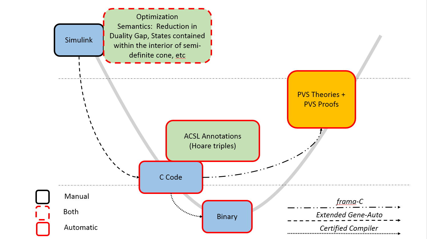
Figure 1: Visualization of autocoding and verification process For Optimization Algorithms

Existing work already provides for the automatic generation of embedded convex optimization code [10]. Given that proofs of high-level functional properties of interior point algorithms do exist, we want to generate the same proof that is sound for the implementation, and expressed in a formal specification language embedded in the code as comments. One of the key ingredients that made credible autocoding applicable for control systems [24] is that the ellipsoid sets generated by synthesizing quadratic Lyapunov functions are relatively easy to reason about even on the code level. The semantics of interior point algorithms, however, do not rely on simple quadratic invariants. The invariant obtained from the proof of good behavior of interior point algorithms is generated by a logarithmic function. This same logarithmic function can also be used in showing the optimization algorithm terminates in within a specified time. This function, is not provided, is perhaps impossible to synthesize from using existing code analysis techniques on the optimization source code. In fact nearly all existing code analyzers only handle linear properties with the notable exception in [21].

3 Program Verification

In this section, we introduce some concepts from program verification that we use later in the paper. The readers who are already familiar with Hoare logic and axiomatic semantics should skip ahead to the next section.

3.1 Axiomatic Semantics

One of the classic paradigms in formal verification of programs is the usage of axiomatic semantics. In axiomatic semantics, the semantics or mathematical meanings of a program is based on the relations between the logic predicates that hold true before and after a piece of code is executed. The program is said to be partially correct if the logic predicates holds throughout the execution of the program. For example, given the simple while loop program in figure 2,

⬇

1le (x*x>0.5)

2 x=0.9*x;

3end

Figure 2: A while loop Program

if we assume the value of variable $\displaystyle x$ belongs to the set $\displaystyle\left[-1,1\right]$ before the execution of the while loop, then the logic predicate x*x<=1 holds before, during and after the execution of the while loop. The predicate that holds before the execution of a block of code is referred to as the pre-condition. The predicate that holds after the execution of a block of code is referred to as the post-condition. Whether a predicate is a pre or post-condition is contextual since its dependent on the block of code that its mentioned in conduction with. A pre-condition for one line of code can be the post-condition for the previous line of the code. A predicate that remains constant i.e. holds throughout the execution of the program is called an invariant. For example, the predicate x*x<=1 is an invariant for the while loop. However the predicate x*x>=0.9 is not an invariant since it only holds during a subset of the total execution steps of the loop.

The invariants can be inserted into the code as comments. We refer to these comments as code specifications or annotations. For example, inserting the predicate x*x<=1 into the program in figure 2 results in the annotated program in figure 3. The pseudo Matlab specification language used to express the annotations in figure 3 is modelled after ANSI/ISO C Specification Language (ACSL [2]), which is an existing formal specification language for C programs. The pre and post-conditions are denoted respectively using ACSL keywords requires and ensures. The annotations are captured within comments denoted by the Matlab comment symbol %%.

⬇

1%% requires x*x<=1; ensures x*x<=1;

2while (x*x>0.5)

3 x=0.9*x;

4end

Figure 3: Axiomatic Semantics for a while loop Program

Throughout the rest of the paper, we use this pseudo Matlab specification language in the annotations of the example convex optimization program. Other logic keywords from ACSL, such as exists, forall and assumes are also transferred over and they have their usual meanings.

3.2 Hoare Logic

We now introduce a formal system of reasoning about the correctness of programs, that follows the axiomatic semantics paradigm, called Hoare Logic [7]. The main structure within Hoare logic is the Hoare triple. Let $\displaystyle P$ be a pre-condition for the block of code $\displaystyle C$ and let $\displaystyle Q$ be the post-condition for $\displaystyle C$. We can express the annotated program in 3 as a Hoare triple denoted by $\displaystyle\left\{P\right\}C\left\{Q\right\}$, in which both $\displaystyle P$ and $\displaystyle Q$ represent the invariant x*x<=1 and $\displaystyle C$ is the while loop. The Hoare triples is partially correct if $\displaystyle P$ hold true for some initial state $\displaystyle\sigma$, and $\displaystyle Q$ holds for the new state $\displaystyle\sigma^{\prime}$ after the execution of $\displaystyle C$. For total correctness, we also need prove termination of the execution of $\displaystyle C$.

Hoare logic includes a set of axioms and inference rules for reasoning about the correctness of Hoare triples for various program structures of a generic imperative programming language. Example program structures include loops, branches, jumps, etc. In this paper, we only consider while loops. For example, a Hoare logic axiom for the while loop is

$$\frac{\left\{P\wedge B\right\}C;\left\{P\right\}}{\left\{P\right\}\textrm{while }B\textrm{ do }C\textrm{ done }\left\{\neg B\wedge P\right\}}.$$ (1)

Informally speaking, the axioms and inference rules should be interpreted as follows: the formula above the horizontal line implies the formula below that line. From (1), note that the predicate $\displaystyle P$ holds before and after the while loop. We typically refer to this type of predicate as an inductive invariant. Inductive invariants require proofs as they are properties that the producer of the code is claiming to be true. For the while loop, according the axiom in (1), we need to show that the predicate $\displaystyle P$ holds in every iteration of the loop. In contrast, axiomatic semantics also allows predicates that are essentially assumptions about the state of the program. This is especially useful in specifying properties about the inputs. For example, the variable x in figure 3 is assumed to have an value between $\displaystyle-1$ and $\displaystyle 1$. The validity of such property cannot be proven since it is an assumption. This type of invariant is referred to as an assertion. In our example, the assertion x<=1 && x>=-1 is necessary for proving that x*x<=1 is an inductive invariant of the loop.

For this paper, we use some basic inferences rules from Hoare logic, which are listed in table 1.

$$\frac{\left\{P_{1}\Rightarrow P_{2}\right\}C\left\{Q_{1}\Rightarrow Q_{2}\right\}}{\left\{P_{1}\right\}C\left\{Q_{2}\right\}}$$ (2)	$$\frac{\left\{P\right\}C_{1}\left\{Q\right\};\left\{Q\right\}C_{2}\left\{W\right\}}{\left\{P\right\}C_{1};C_{2}\left\{W\right\}}$$ (3)
$$\frac{}{\left\{P\right\}SKIP\left\{P\right\}}$$ (4)	$$\frac{}{\left\{P[e/x]\right\}x:=expr\left\{P\right\}}$$ (5)
$$\frac{}{\left\{P\right\}x:=expr\left\{\exists x_{0}\left(x=expr\left[x_{0}/x\right]\right)\wedge P\left[x_{0}/x\right]\ \right\}}$$ (6)

Table 1: Axiomatic Semantics Inference Rules for a Imperative Language

The consequence rule in (2) is useful whenever a stronger pre-condition or weaker post-condition is needed. By stronger, we meant the set defined by the predicate is smaller. By weaker, we mean precisely the opposite. The substitution rules in (5) and (6) are used when the code is an assignment statement. The weakest pre-condition $\displaystyle P[x/expr]$ in (5) means $\displaystyle P$ with all instances of the expression $\displaystyle expr$ replaced by $\displaystyle x$. For example, given a line of code y=x+1 and a known weakest pre-condition x+1<=1, we can deduct that y<=1 is a correct post-condition using the backward substitution rule. Although usually (5) is used to compute the weakest pre-condition from the known post-condition. Alternatively the forward propagation rule in (6) is used to compute the strongest post-condition. The skip rule in (4) is used when executing the piece of code does not change any variables in the pre-condition $\displaystyle P$.

3.3 Proof Checking

The utility of having the invariants in the code is that finding the invariants is in general more difficult than checking that given invariants are correct. By expressing and translating the high-level functional properties and their proofs onto the code level in the form of invariants, we can verify the correctness of the optimization program with respect to its high-level functional properties using a proof-checking procedure i.e. by verifying each use of a Hoare logic rule.

4 Semi-Definite Programming and the Interior Point Method

In this section, we give an overview of the Semi-Definite Programming (SDP) problem. The readers who are already familiar with interior point method and convex optimization can skip ahead to the next section. The notations used in this section are as follows: let $\displaystyle A=(a_{i,j})_{1\leq i,j\leq n},B\in\mathbb{R}^{n\times n}$ be two matrices and $\displaystyle a,b\in\mathbb{R}^{n}$ be two column vectors. $\displaystyle\operatorname{Tr}\left(A\right)=\sum_{i=1}^{n}a_{i,i}$ denotes the trace of matrix $\displaystyle A$. $\displaystyle\langle\cdot,\cdot\rangle$ denotes an inner product, defined in $\displaystyle\mathbb{R}^{n\times n}\times\mathbb{R}^{n\times n}$ as $\displaystyle\langle A,B\rangle:=\operatorname{Tr}\left(B^{\textrm{T}}A\right)$ and in $\displaystyle\mathbb{R}^{n}\times\mathbb{R}^{n}$ as $\displaystyle\langle a,b\rangle:=a^{\textrm{T}}b$. The Frobenius norm of $\displaystyle A$ is defined as $\displaystyle\|A\|_{F}=\sqrt{\langle A,A\rangle}$. The symbol $\displaystyle\mathbb{S}^{n}$ denotes the space of symmetric matrices of size $\displaystyle n\times n$. The space of $\displaystyle n\times n$ symmetric positive-definite matrices is denoted as $\displaystyle\mathbb{S}^{n+}=\left\{S\in\mathbb{S}^{n}|\forall x\in\mathbb{R}^{n}\setminus\{0\},x^{\textrm{T}}Sx>0\right\}$. If $\displaystyle A$ and $\displaystyle B$ are symmetric, $\displaystyle A\prec B$ (respectively $\displaystyle A\succ B$) denotes the positive (respectively negative)-definiteness of matrix $\displaystyle B-A$. The symbol $\displaystyle I$ denotes an identity matrix of appropriate dimension. For $\displaystyle X,Z\in\mathbb{S}^{n+}$, some basic properties of matrix derivative are $\displaystyle\displaystyle\frac{\partial\operatorname{Tr}\left(XZ\right)}{\partial X}=Z^{\textrm{T}}=Z$ and $\displaystyle\displaystyle\frac{\partial\operatorname{det}\left(X\right)}{\partial X}=\operatorname{det}\left(X\right)^{-1}\left(X^{-1}\right)^{\textrm{T}}=\operatorname{det}\left(X\right)^{-1}X^{-1}$.

4.1 SDP Problem

Let $\displaystyle n,m\in\mathbb{N}$, $\displaystyle F_{0}\in\mathbb{S}^{n+}$, $\displaystyle F_{1},F_{2},\ldots,F_{m}\in\mathbb{S}^{n}$, and $\displaystyle b=\begin{bmatrix}b_{1}&b_{2}&\ldots&b_{m}\end{bmatrix}^{\textrm{T}}\in\mathbb{R}^{m}$. Consider a SDP problem of the form in (7). The linear objective function $\displaystyle\langle F_{0},Z\rangle$ is to be maximized over the intersection of positive semi-definite cone $\displaystyle\left\{Z\in\mathbb{S}^{n}|Z\succeq 0\right\}$ and a convex region defined by $\displaystyle m$ affine equality constraints.

$$\underset{Z}{\text{sup}} \langle F_{0},Z\rangle,$$ (7)

subject to $$\langle F_{i},Z\rangle+b_{i}=0, i=1,\ldots,m$$

$$Z\succeq 0.$$

Note that a SDP problem can be considered as a generalization of a linear programming (LP) problem. To see this, let $\displaystyle Z=\operatorname{Diag}{\left(z\right)}$ where $\displaystyle z$ is the standard LP variable.

We denote the SDP problem in (7) as the dual form. Closely related to the dual form, is another SDP problem as shown in (8), called the primal form. In the primal formulation, the linear objective function $\displaystyle\langle b,p\rangle$ is minimized over all vectors $\displaystyle p=\begin{bmatrix}p_{1}&\ldots&p_{m}\end{bmatrix}^{\textrm{T}}\in\mathbb{R}^{m}$ under the semi-definite constraint $\displaystyle F_{0}+\sum_{i=1}^{m}p_{i}F_{i}\preceq 0$. Note the introduction in (8) of a variable $\displaystyle X=-F_{0}-\sum_{i=1}^{m}p_{i}F_{i}$ such that $\displaystyle X\succeq 0$, which is not strictly needed to express the problem, but is used in later developments.

$$\underset{p,X}{\text{inf}} \langle b,p\rangle$$ (8)

subject to $$F_{0}+\sum_{i=1}^{m}p_{i}F_{i}+X=0$$

$$X\succeq 0.$$

We assume the primal and dual feasible sets defined as

$$\begin{array}[]{l}\displaystyle\mathcal{F}^{p}=\left\{X|X=-F_{0}-\sum_{i=1}^{m}p_{i}F_{i}\succeq 0,p\in\mathbb{R}^{m}\right\},\\ \displaystyle\mathcal{F}^{d}=\left\{Z|\langle F_{i},Z\rangle+b_{i}=0,Z\succeq 0\right\}\end{array}$$ (9)

are not empty. Under this condition, for any primal-dual pair $\displaystyle(X,Z)$ that belongs to the feasible sets in (9), the primal cost $\displaystyle\langle b,p\rangle$ is always greater than or equal to the dual cost $\displaystyle\langle F_{0},Z\rangle$. The difference between the primal and dual costs for a feasible pair $\displaystyle(X,Z)$ is called the duality gap. The duality gap is a measure of the optimality of a primal-dual pair. The smaller the duality gap, the more optimal the solution pair $\displaystyle(X,Z)$ is. For (8) and (7), the duality gap is the function

$$G(X,Z)=\operatorname{Tr}\left(XZ\right).$$ (10)

Indeed,

$$\displaystyle\operatorname{Tr}\left(XZ\right) \displaystyle= \displaystyle\operatorname{Tr}\left(\left(-F_{0}-\sum_{i=1}^{m}p_{i}F_{i}\right)Z\right)=-\operatorname{Tr}\left(F_{0}Z\right)-\sum_{i=1}^{m}p_{i}\operatorname{Tr}\left(F_{i}Z\right)$$

$$\displaystyle= \displaystyle\langle b,p\rangle-\langle F_{0},Z\rangle.$$

Finally, if we assume that both problems are strictly feasible i.e. the sets

$$\begin{array}[]{l}\displaystyle\mathcal{F}^{p^{\prime}}=\left\{X|X=-F_{0}-\sum_{i=1}^{m}p_{i}F_{i}\succ 0,p\in\mathbb{R}^{m}\right\},\\ \displaystyle\mathcal{F}^{d^{\prime}}=\left\{Z|\langle F_{i},Z\rangle+b_{i}=0,Z\succ 0\right\}\end{array}$$ (11)

are not empty, then there exists an optimal primal-dual pair $\displaystyle(X^{*},Z^{*})$ such that

$$\operatorname{Tr}\left(X^{*}Z^{*}\right)=0.$$ (12)

Moreover, the primal and dual optimal costs are guaranteed to be finite. The condition in (12) implies that for strictly feasible problems, the primal and dual costs are equal at their respective optimal points $\displaystyle X^{*}$ and $\displaystyle Z^{*}$. Note that in the strictly feasible problem, the semi-definite constraints become definite constraints.

The canonical way of dealing with constrained optimization is by first adding to the cost function a term that increases significantly if the constraints are not met, and then solve the unconstrained problem by minimizing the new cost function. This technique is commonly referred to as the relaxation of the constraints. For example, lets assume that the problems in (8) and (7) are strictly feasible. The positive-definite constraints $\displaystyle X\succ 0$ and $\displaystyle Z\succ 0$, which defines the interior of a pair of semi-definite cones, can be relaxed using an indicator function $\displaystyle I(X,Z)$ such that

$$I:\left(X,Z\right)\rightarrow\left\{\begin{array}[]{lc}0,&X\succ 0,Z\succ 0\\ +\infty,&\textrm{otherwise}\end{array}\right.$$ (13)

The intuition behind relaxation using an indicator function is as follows. If the primal-dual pair $\displaystyle(X,Z)$ approaches the boundary of the interior region, then the indicator function $\displaystyle I(X,Z)$ approaches infinity, thus incurring a large penalty on the cost function.

The indicator function in (13) is not useful for optimization because it is not differentiable. Instead, the indicator function can be replaced by a family of smooth, convex functions $\displaystyle B(X,Z)$ that not only approximate the behavior of the indicator function but are also self-concordant. We refer to these functions as barrier functions. A scalar function $\displaystyle F:\mathbb{R}\rightarrow\mathbb{R}$, is said to be self-concordant if it is at least three times differentiable and satisfies the inequality

$$|F^{\prime\prime\prime}(x)|\leq 2F^{\prime\prime}(x)^{\frac{3}{2}}.$$ (14)

The concept of self-concordance has been generalized to vector and matrix functions, thus we can also find such functions for the positive-definite variables $\displaystyle X$ and $\displaystyle Z$. Here we state, without proof, the key property of self-concordant functions.

Property 1

Functions that are self-concordant can be minimized in polynomial time to a given non-zero accuracy using a Newton type iteration [16].

Examples of self-concordant functions include linear functions, quadratic functions, and logarithmic functions. A valid barrier function for the semi-definite constraints from (8) and (7) is

$$B(X,Z)=-\log{\operatorname{det}\left(X\right)}-\log{\operatorname{det}\left(Z\right)}.$$ (15)

5 An Interior Point Algorithm and Its Properties

We now describe an example primal-dual interior point algorithm. We focus on the key property of convergence. We show its usefulness in constructing the inductive invariants to be applied towards documenting the software implementation. The algorithm is displayed in table 2 and is based on the work in [14].

5.1 Details of the Algorithm

The algorithm in table 2 is consisted of an initialization routine and a while loop. The operator length is used to compute the size of the input problem data. The operator ^^-1 represents an algorithm such as QR decomposition that returns the inverse of the matrix. The operator ^^0.5 represents an algorithm such as Cholesky decomposition that computes the square root of the input matrix. The operator lsqr represents a least-square QR factorization algorithm that is used to solve linear systems of equation of the form $\displaystyle Ax=b$. With the assumption of real algebra, all of these operators return exact solutions.

In the initialization part, the states $\displaystyle X$, $\displaystyle Z$ and $\displaystyle p$ are initialized to feasible values, and the input problem data are assigned to constants $\displaystyle F_{i},i=1,\ldots,m$. The term feasible here means that $\displaystyle X$, $\displaystyle Z$, and $\displaystyle p$ satisfies the equality constraints of the primal and dual problems. We discuss more about the efficiency of the initialization process later on.

The while loop is a Newton iteration that computes the zero of the derivative of the potential function

$$\phi(X,Z)=\left(n+\nu\sqrt{n}\right)\log{\operatorname{Tr}\left(XZ\right)}-\log{\operatorname{det}\left(XZ\right)}-n\log{n},$$ (16)

in which $\displaystyle\nu$ is a positive weighting factor. Note that the potential function is a weighted sum of the primal-dual cost gap and the barrier function potential. The weighting factor $\displaystyle\nu$ is used in computing the duality gap reduction factor $\displaystyle\sigma\equiv\frac{n}{n+\nu\sqrt{n}}$. A larger $\displaystyle\nu$ implies a smaller $\displaystyle\sigma$, which then implies a shorter convergence time. For our algorithm, since we use a fix-step size of $\displaystyle 1$, a small enough $\displaystyle\sigma$ combined with the newton step could result in a pair of $\displaystyle X$ and $\displaystyle Z$ that no longer belong to the interior of the positive-semidefinite cone. In the running example, we have $\displaystyle\nu=0.4714$. While this choice of $\displaystyle\nu$ doubled the number of iterations of the running example compared to the typical choice of $\displaystyle\nu=1$, however it is critical in satisfying the invariants of the while loop that are introduced later this paper.

Algorithm 1. MZ Short-Path Primal-Dual Interior Point Algorithm

Input: $\displaystyle F_{0}\succ 0$, $\displaystyle F_{i}\in\mathbb{S}^{n},i=1,\ldots,m$, $\displaystyle b\in\mathbb{R}^{m}$

$\displaystyle\epsilon$: Optimality desired

1. Initialize:

Compute $\displaystyle Z$ such that $\displaystyle\langle F_{i},Z\rangle=-b_{i},i=1,\ldots,m$;

Let $\displaystyle X\leftarrow\hat{X}$; // $\displaystyle\hat{X}$ is some positive-definite matrix

Compute $\displaystyle p$ such that $\displaystyle\sum_{i}^{m}p_{i}F_{i}=-X_{0}-F_{0}$;

Let $\displaystyle\mu\leftarrow\frac{\langle X,Z\rangle}{n}$;

Let $\displaystyle\sigma\leftarrow 0.75$;

Let $\displaystyle n\leftarrow\operatorname{length}{F_{i}}$, $\displaystyle m\leftarrow\operatorname{length}{b_{i}}$;

2. while $\displaystyle n\mu>\epsilon$ {

3.       Let $\displaystyle\phi_{-}\leftarrow\langle X,Z\rangle$;

4.       Let $\displaystyle T_{inv}\leftarrow Z^{0.5}$;

5.       Let $\displaystyle T\leftarrow T_{inv}^{-1}$;

6.       Compute $\displaystyle(\Delta Z,\Delta X,\Delta p)$ that satisfies (17);

7.       Let $\displaystyle Z\leftarrow Z+\Delta Z$, $\displaystyle X\leftarrow X+\Delta X$, $\displaystyle p\leftarrow p+\Delta p$;

8.       Let $\displaystyle\phi\leftarrow\langle X,Z\rangle$;

9.       Let $\displaystyle\mu\leftarrow\frac{\langle X,Z\rangle}{n}$;

10.       if ($\displaystyle\phi-\phi_{-}>0$) {

11.            $\displaystyle\operatorname{return}{}$;

}

}

Table 2: Primal-Dual Short Path Interior Point Algorithm

Let symbol $\displaystyle T=Z^{-0.5}$ and $\displaystyle T_{inv}$ denotes the inverse of $\displaystyle T$. The while loop solves the set of matrix equations

$$\langle F_{i},\Delta Z\rangle =0$$ (17)

$$\sum_{i}^{m}\Delta p_{i}F_{i}+\Delta X =0$$

$$\frac{1}{2}\left(T\left(Z\Delta X+\Delta ZX\right)T_{inv}+T_{inv}\left(\Delta XZ+X\Delta Z\right)T\right) =\sigma\mu I-T_{inv}XT_{inv}.$$

for the Newton-search directions $\displaystyle\Delta Z$, $\displaystyle\Delta X$ and $\displaystyle\Delta p$. The first two equations in (17) are obtained from a Taylor expansion of the equality constraints from the primal and dual problems. These two constraints formulates the feasibility sets as defined in Eq (9). The last equation in (17) is obtained by setting the Taylor expansion of the derivative of (16) equal to $\displaystyle 0$, and then applying the symmetrizing transformation

$$\begin{array}[]{lc}\displaystyle H_{T}:M\rightarrow\frac{1}{2}\left(TMT^{-1}+\left(TMT^{-1}\right)^{\textrm{T}}\right),&T=Z^{-0.5}\end{array}$$ (18)

to the result. To see this, note that derivative of (16) is $\displaystyle\left[\begin{array}[]{cc}XZ-\frac{n}{n+\nu\sqrt{n}}\frac{\operatorname{Tr}\left(XZ\right)}{n}I&\end{array}\right.$ $\displaystyle\left.\begin{array}[]{c}ZX-\frac{n}{n+\nu\sqrt{n}}\frac{\operatorname{Tr}\left(XZ\right)}{n}I\end{array}\right]$.

The transformation in (18) is necessary to guarantee the solution $\displaystyle\Delta X$ is symmetric. The parameter $\displaystyle\sigma$, as mentioned before, can be interpreted as a duality gap reduction factor. To see this, note that the 3rd equation in (17) is the result of applying Newton iteration to solve the equation $\displaystyle XZ=\sigma\mu I$. With $\displaystyle\sigma\in(0,1)$, the duality gap $\displaystyle\operatorname{Tr}\left(XZ\right)=n\sigma\mu$ is reduced after every iteration. The choice of $\displaystyle T$ in (18) is taken from [13] and is called the Monteiro-Zhang (MZ) direction. Many of the Newton search directions from the interior-point method literature can be derived from an appropriate choice of $\displaystyle T$. The M-Z direction also guarantees an unique solution $\displaystyle\Delta X$ to (17). The while loop then updates the states $\displaystyle X,Z,p$ with the computed search directions and computes the new normalized duality gap. The aforementioned steps are repeated until the duality gap $\displaystyle n\mu$ is less than the desired accuracy $\displaystyle\epsilon$.

5.2 High-level Functional Property of the Algorithm

The key high-level functional property of the interior point algorithm in 2 is an upper bound on the worst case computational time to reach the specified duality gap $\displaystyle\epsilon>0$. The convergence rate is derived from a constant reduction in the potential function in (16) [11] after each iteration of the while loop.

Given the potential function in (16), the following result gives us a tight upper bound on the convergence time of our running example.

Theorem 5.1

Let $\displaystyle X_{-}$, $\displaystyle Z_{-}$, and $\displaystyle p_{-}$ denote the values of $\displaystyle X$, $\displaystyle Z$, and $\displaystyle p$ in the previous iteration. If there exist a constant $\displaystyle\delta>0$ such that

$$\phi(X_{-},Z_{-})-\phi(X,Z)\geq\delta,$$ (19)

then Algorithm 2 will take at most $\displaystyle\mathcal{O}\left(\sqrt{n}\log{\epsilon^{-1}\operatorname{Tr}\left(X_{0}Z_{0}\right)}\right)$ iterations to converge to a duality gap of $\displaystyle\epsilon$,

For safety-critical applications, it is important for the optimization program implementation to have a rigorous guarantee of convergence within a specified time. Assuming that the required precision $\displaystyle\epsilon$ and the problem data size $\displaystyle n$ are known a priori, we can guarantee a tight upper bound on the optimization algorithm if the function $\displaystyle\phi$ satisfies (19). For the running example, this is indeed true. We have the following result.

Theorem 5.2

There exists a constant $\displaystyle\delta>0$ such that theorem 5.1 holds.

The proof of theorem 5.2 is not shown here for the sake of brevity but it is based on proofs already available in the interior point method literature (see [8] and [18]).

Using theorems 5.1 and 5.2, we can conclude that the algorithm in table 2, at worst, converges to the $\displaystyle\epsilon$-optimal solution linearly. For documenting the while loop portion of the implementation, however we need to construct an inductive invariant of the form

$$0\leq\phi(X,Z)\leq c,$$ (20)

in which $\displaystyle c$ is a positive scalar. While the potential function in (16) is useful for the construction of the algorithm in table 2, but it is not non-negative. To construct an invariant in the form of (20), instead of using (16), consider

$$\phi(X,Z)=\log{\operatorname{Tr}\left(XZ\right)},$$ (21)

which is simply the log of the duality gap function.

Theorem 5.3

The function in (21) satisfies theorems 5.1 and 5.2.

An immediate implication of theorem 5.3 is that $\displaystyle\operatorname{Tr}\left(XZ\right)$ converges to $\displaystyle 0$ linearly i.e. $\displaystyle\displaystyle\exists\kappa\in(0,1)$ such that $\displaystyle\operatorname{Tr}\left(XZ\right)\leq\kappa\operatorname{Tr}\left(X_{-}Z_{-}\right)$, in which $\displaystyle X_{-}$ and $\displaystyle Z_{-}$ are values of $\displaystyle X$ and $\displaystyle Z$ at the previous iteration. Using $\displaystyle\operatorname{Tr}\left(XZ\right)$, we can construct the invariant from (20) and another invariant $\displaystyle\phi-\kappa\phi_{-}<0$ to express the convergence property from theorem 5.1.

Additionally, there is one other invariant to be documented for the while loop. The first one is the positive-definiteness of the states $\displaystyle X$ and $\displaystyle Z$. We need to show that the initial $\displaystyle X$ and $\displaystyle Z$ belongs to a positive-definite cone. We also need to show that they are guaranteed to remain in that cone throughout the execution of the while loop. This inductive property is directly obtained from the constraints on the variables $\displaystyle X$ and $\displaystyle Z$. It is also used to show that the duality gap $\displaystyle\operatorname{Tr}\left(XZ\right)$ is positive.

6 Running Example

In this section, we introduce a basic optimization problem and a matlab program that solves the problem using the interior-point algorithm in table 2.

6.1 Input Problem

The input data is obtained from a generic optimization problem taken from systems and control. The details of the original problem is skipped here as it has no bearing on the main contribution of this article. We do like to mention that the matrices $\displaystyle F_{i},i=0,\ldots,3$ are computed from the original problem using the tool Yalmip [9].

6.2 Matlab Implementation

The Matlab implementation contains some minor differences from the algorithm description. The first is that, in the Matlab implementation, the current values of $\displaystyle X$, $\displaystyle Z$, $\displaystyle p$ are assigned to the variables $\displaystyle X_{-}$, $\displaystyle Z_{-}$, and $\displaystyle p_{-}$ at the beginning of the while loop. Note that the variables $\displaystyle X_{-}$, $\displaystyle Z_{-}$, and $\displaystyle p_{-}$ are denoted by Xm, Zm and pm respectively in the Matlab code. Because of that, steps 3 to 6 of algorithm in Table 2 are executed with the variables $\displaystyle X_{-}$, $\displaystyle Z_{-}$, and $\displaystyle p_{-}$ instead of $\displaystyle X$, $\displaystyle Z$, and $\displaystyle p$. Accordingly, step 7 becomes $\displaystyle Z\leftarrow Z_{-}+\Delta Z_{-}$, $\displaystyle X\leftarrow X_{-}+\Delta X_{-}$, $\displaystyle p\leftarrow p_{-}+\Delta p_{-}$. This difference is the result of the need to have the invariant of the form $\displaystyle\phi\left(X,Z\right)\leq\kappa\phi\left(X_{-},Z_{-}\right)$ for $\displaystyle\kappa\in(0,1)$, which is important since it expresses the fast convergence property from theorem 5.1.

7 Annotating an Optimization Program for Deductive Verification

In this section, we discuss, line by line, an example of a fully-annotated optimization program that is based on the interior-point algorithm in figure 2. The fully-annotated program represents a claim of proof that the code also conforms to certain safety or liveness property of the algorithm. The claim of proof need to be verified by a proof-checking program, which we called the backend. The annotated program was written in the Matlab language and the Hoare logic style annotations were inserted manually. Matlab was chosen as the implementation language because of its compactness and readability. For the automation of the process i.e. the credible autocoding framework, we shall choose a realistic target language such as C that is more acceptable for formal analysis and verification.

The annotation process starts with the selection of a safety or liveness property of the interior-point algorithm in which the code originates from. The chosen property is formalized and then translated into invariants and then inserted into the code as Hoare logic pre/post conditions. For the example optimization program, the invariant that encode the property of bounded execution time of the program is $\displaystyle\phi-0.76\phi_{-}<0$. Various additional proof elements are inserted into the code, also in the form of Hoare logic style pre/post-conditions, to allow easy automation of the proof-checking process. The amount of additional proof elements needed is dependent on the capability of the backend. Lastly, by using the Hoare logic rules, the entire program is populate with pre/post-conditions, thus resulting in the fully-annotated code.

The rest of this section is organized as follows. First we give the example Matlab implementation and a description of the non-standard Matlab functions used in the code. Second, we give a description of the annotation language used in expressing the invariants and assertions. Finally, we give a detailed description of all the Hoare triples in the fully-annotated example.

7.1 Matlab Implementation

The example implementation uses three non-standard Matlab operators vecs, mats and krons. These operators are used to transform the matrix equations in(17) into matrix vector equations in the form $\displaystyle Ax=b$. For more details about these operator, please refer to the appendix. The symbol ’ denotes Matlab’s transpose function.

⬇

1[1, 0; 0, 0.1];

2F1=[-0.750999 0.00499; 0.00499 0.0001];

3F2=[0.03992 -0.999101; -0.999101 0.00002];

4F3=[0.0016 0.00004; 0.00004 -0.999999];

5b=[0.4; -0.2; 0.2];

6n=length(F0);

7m=length(b);

8F=[vecs(F1); vecs(F2); vecs(F3)];

9Ft=F’;

10Z=mats(lsqr(F,-b),n);

11X=[0.3409 0.2407; 0.2407 0.9021];

12epsilon=1e-8;

13sigma=0.75;

14phi=trace(X*Z);

15phim=1/0.75*phi;

16P=mats(lsqr(Ft,vecs(-X-F0)),n);

17p=vecs(P);

18while (phi>epsilon) {

19 Xm=X;

20 Zm=Z;

21 pm=p;

22 mu=trace(Xm*Zm)/n;

23 Zh=Zm^(0.5);

24 Zhi=Zh^(-1);

25 G=krons(Zhi,Zh’*Xm,n,m);

26 H=krons(Zhi*Zm,Zh’,n,m);

27 r=sigma*mu*eye(n,n)-Zh*Xm*Zh;

28 dZm=lsqr(F,zeros(m,1));

29 dXm=lsqr(H, vecs(r)-G*dZm);

30 dpm=lsqr(Ft,-dXm);

31 p=pm+dpm

32 X=Xm+mats(dXm,n);

33 Z=Zm+mats(dZm,n);

34 phim=trace(Xm*Zm);

35 phi=trace(X*Z);

36 mu=trace(X*Z)/n;

37}

Figure 4: Optimization Program in Matlab

The program is divided into two parts. The first part, which we call the initialization part, assigns the data of the input optimization problem to memory and initializes the variables to be optimized. The second part, which is the while loop, executes the interior-point algorithm to solve the input optimization problem.

7.2 Annotation Language

The fully-annotated example is displayed in section 12.2 of the appendix. The annotations are expressed using a pseudo Matlab specification language (MSL) that is similar, in features, to the ANSI/ISO C Specification Language (ACSL) for C programs [4], Like in ACSL, the keywords requires and ensures denote a pre and post-condition statement respectively. A MSL contract, like the ACSL contract, is used to express a Hoare triple. For example, the MSL contract displayed in figure 5 can be parsed as the Hoare triple $\displaystyle\left\{P\right\}C;\left\{Q\right\}$.

⬇

1% requires Pensures Q

2{

3 C;

4}

Figure 5: An ACSL-like Contract

A block of code can have more than one contract. For example, as shown in figure 6, the two MSL contracts translates to the Hoare triples

$$\left\{P_{i}\right\}C;\left\{Q_{i}\right\},i=1,2.$$ (22)

⬇

1% requires P1ensures Q2

2

3% requires P2

4% ensures Q2

5{

6 C;

7}

Figure 6: Multiple Contracts

A block of empty code can also have contract. For example, the formula $\displaystyle P\Rightarrow Q$ can be expanded into a Hoare triple $\displaystyle\left\{P\right\}empty;\left\{Q\right\}$, which is expressed using the MSL contract in figure 7.

⬇

1% requires Pensures Q

2{

3 % empty;

4}

Figure 7: Contract for an empty code

Remark 1

The block of empty code appear in our annotated program, for example when we expand the post-condition of Hoare triple such as

$$\left\{P\right\}C;\left\{Q_{1}\Rightarrow Q_{2}\right\}$$ (23)

into an additional Hoare triple. This transformation results in (23) being expanded into two Hoare triples

$$\left\{P\right\}C;\left\{Q_{1}\right\}$$ (24)

and

$$\left\{Q_{1}\right\}empty;\left\{Q_{2}\right\}.$$ (25)

The main reason to expand a Hoare triple into multiple ones is to simplify the automation of the proof-checking process. The choice in expanding is arbitrary as it is dependent on the capability of the backend. For example, in the case of (23), it is possible that the backend can verify (24) and (25) separately but not (23) without human input. Practically speaking, by reducing the complexity in the verification of an individual Hoare triple in exchange for an increase in the total number of Hoare triples, the proof-checking process usually become easier to automate.

A contract can have more than one pre-condition statement as shown in figure 8. The pre-condition statements are combined into a single pre-condition $\displaystyle P$ conjunctively when the contract is parsed as a Hoare triple. For example, the contract in figure 8 expresses the Hoare triple $\displaystyle\left\{P_{1}\wedge P_{2}\right\}empty;\left\{Q\right\}$.

⬇

1% requires P_1requires P_2

2% ensures Q

3{

4 C;

5}

Figure 8: Contract for an empty code

The logic comparison operator $\displaystyle>$ is overloaded to express $\displaystyle\succ$. The function smat is the inverse of the function svec. The function svec is similar to the symmetric vectorization function vecs but with a multiplication factor of $\displaystyle 2$. For example, the expression smat([0.4;-0.2;0.2] returns the matrix

$$\begin{bmatrix}0.4&-0.1\cr-0.1&0.2\end{bmatrix}.$$ (26)

7.3 Functions with Verified Contracts

Certain functions used in the example program comes by default with MSL contracts to ensures the regularity of the inputs and outputs to the functions. These annotations are implicit since they are assumed to be correct.

For example, the square root function and the inverse function denoted by the symbols 0̂.5 and -̂1.0 respectively, comes by default with the properties that the input matrix is symmetric positive-definite and the output is also symmetric positive-definite.

⬇

1% requires Zm>0;ensures Zh>0;

2Zh=Zm^(0.5);

3% requires Zh>0;

4% ensures Zhi>0;

5Zhi=Zh^(-1)

The function lsqr comes by default with the post-condition which stipulates that the matrix-vector product of the first argument of the function and the output of the function is equal to the second argument of the function.

⬇

1% ensures F*y==-b;lsqr(F,-b);

The function vecs by default comes with the pre-condition that the input argument to the function is a symmetric matrix.

⬇

1% requires P==transpose(P);vecs(P);

The function mats, as displayed below, requires that $\displaystyle x\in\mathbb{R}^{\frac{n\left(n+1\right)}{2}}$ and ensures that the output $\displaystyle X$ is a symmetric matrix of size $\displaystyle n$.

⬇

1% requires n>=1;requires type(x)==vector(n/2*(n+1));

2% ensures type(X)==symmetric_matrix(n);

3X=mats(x,n);

7.4 Annotated Code

For the analysis and discussion of the annotations, the fully-annotated example is split into multiple parts and each part is displayed in a separate figure and discussed in a separate subsection. In those figures, every MSL contract is assigned a pair of numbers $\displaystyle(n,m)$, which indicates the $\displaystyle m$th contract of the $\displaystyle n$th block of code of the figure. The Hoare triple expressed by the contract with a label of $\displaystyle(n,m)$ is denoted as

$$\mathcal{H}_{n,m}:=\left\{P_{n,m}\right\}C_{n};\left\{Q_{n,m}\right\}.$$ (27)

For example, in figure 7.4, $\displaystyle\mathcal{H}_{1,1}$ is the Hoare triple $\displaystyle\left\{x>0\right\}x=y;\left\{y>0\right\}$, with $\displaystyle P_{1,1}$ being the pre-condition $\displaystyle x>z$, $\displaystyle C_{1}$ being the line of code y=x-z; and $\displaystyle Q_{1,1}$ being the post-condition $\displaystyle y>0$.

⬇

1% (1,1) requires x>z; ensures y>0;

2

3% (1,2) requires x<0;

4% requires z>0;

5% ensures y<0;

6{

7 y=x-z;

8}

Also in figure 7.4, $\displaystyle\mathcal{H}_{1,2}$ is the Hoare triple $\displaystyle\left\{x<0\wedge z>0\right\}y=x-z;\left\{y<0\right\}$, with $\displaystyle P_{1,2}:=x<0\wedge z>0$, and $\displaystyle Q_{1,2}:=y<0$.

The variables from the program will be referenced using either their programmatic textual representation or their corresponding mathematical symbols. For example, the list of variables phi, phim, dXm, and Xm is the same as the list of symbols $\displaystyle\phi$, $\displaystyle\phi_{-}$, $\displaystyle\Delta_{X_{-}}$, and $\displaystyle X_{-}$ Likewise, the annotations are also referenced using both representations as well. For example, the expression phim=trace(Xm*Zm)/n is equivalent to $\displaystyle\phi_{-}:=\frac{\operatorname{Tr}\left(X_{-}Z_{-}\right)}{n}$. Some expressions from the program such as mats(dXm,n) and mats(dZm,n) are referenced using the more compact symbols $\displaystyle\Delta X_{-}$ and $\displaystyle\Delta Z_{-}$ respectively.

7.5 Proof Checking the Annotations

We assume there exists an automated proof-checking program, which we referred to as the backend, that can be used to verify the Hoare triples in the annotated example. We will not go into much details about the backend other than occasionally discussing some of theories and formulas needed to verify certain annotations.

7.6 Initialization Part I

The first part of initialization code along with its annotations is displayed in figure 9. The annotations described in this subsection of the paper are from that figure unless explicitly states otherwise.

⬇

1% (1,1) ensures F0>0; F0=[1, 0; 0, 0.1];

2}

3% (2,1) ensures transpose(F1)==F1;

4{

5 F1=[-0.750999 0.00499; 0.00499 0.0001];

6}

7% (3,1) ensures transpose(F2)==F2;

8{

9 F2=[0.03992 -0.999101; -0.999101 0.00002];

10}

11% (4,1) ensures transpose(F3)==F3;

12{

13 F3=[0.0016 0.00004; 0.00004 -0.999999];

14}

15% (5,1) ensures smat(b)>0;

16{

17 b=[0.4; -0.2; 0.2];

18}

19F=[vecs(F1); vecs(F2); vecs(F3)];

20% (6,1) ensures Ft==transpose(F);

21{

22 Ft=F’;

23}

24% (7,1) ensures n>=1;

25{

26 n=length(F0);

27}

28% (8,1) ensures m>=1;

29{

30 m=length(b);

31}

Figure 9: Initialization

In $\displaystyle C_{i},i=1,\ldots,5$, the data parameters of the input optimization problem are assigned to the appropriate variables. The inserted post-conditions $\displaystyle P_{i,1},i=1,\ldots,5$ represent regularity conditions on the data parameters of the input problem. The correctness of these post-conditions guarantee that the input optimization problem is well-posed. For example, the post-condition $\displaystyle P_{1,1}$ claims that the variable F0 is positive-definite after the execution of $\displaystyle C_{1}$ in line 2. Another example is $\displaystyle Q_{2,1}$ which claims that after execution of $\displaystyle C_{2}$ in line 4, the variable F1 is a symmetric matrix.

In $\displaystyle C_{6}$ and $\displaystyle C_{y}$, the problem sizes are computed. In our example, the variable m denotes the number of equality constraints in the dual formulation and the variable n denotes the dimensions of the optimization variables $\displaystyle X$ and $\displaystyle Z$. The inserted post-conditions $\displaystyle Q_{6,1}$ and $\displaystyle Q_{7,1}$ checks that the problem sizes are at least one.

7.7 Intialization Part II

The annotations described in this subsection of the paper are from figure 10 unless explicitly states otherwise.

⬇

1% (1,1) ensures Z>0; Z=mats(lsqr(F,-b),n);

2}

3% (2,1) ensures X>0

4

5% (2,2) ensures trace(X*Z)<=0.1;

6{

7 X=[0.3409 0.2407; 0.2407 0.9021];

8}

9% (3,1) requires Z>0 && X>0;

10% ensures trace(X*Z)>0;

11{

12 % empty code

13}

14% (4,1) ensures transpose(P)==P;

15{

16 P=mats(lsqr(Ft,vecs(-X-F0)),n);

17 p=vecs(P);

18}

19% (5,1) ensures epsilon>0

20{

21 epsilon=1e-8;

22}

23% (6,1) ensures sigma==0.75;

24{

25 sigma=0.75;

26}

27% (7,1) requires trace(X*Z)<=0.1;

28% ensures phi<=0.1;

29

30% (7,2) requires trace(X*Z)>0;

31% ensures phi>0;

32

33% (7,3) ensures phi==trace(X*Z);

34{

35 phi=trace(X*Z);

36}

37% (8,1) requires phi>0;

38% ensures phi-0.76/0.75*phi<0;

39{

40 % empty code

41}

42% (9,1) requires phi-0.76/0.75*phi<0;

43% ensures phi-0.76*phim<0;

44{

45 phim=1/0.75*phi;

46}

47% (10,2) ensures mu==trace(X*Z)/n;

48{

49 mu=trace(X*Z)/n;

50}

Figure 10: Initialization Part II

The blocks of code $\displaystyle C_{i},i=1,2$ generate and then assign initial values to variables $\displaystyle X$ and $\displaystyle Z$. The values of variables $\displaystyle X$ and $\displaystyle Z$ need to be positive-definite in order to satisfy the strict feasibility property of the input optimization problem. Furthermore, functions used in the latter part of the program such as 0̂.5 and -̂1 implicitly require the input to be positive-definite. To check if $\displaystyle X$ and $\displaystyle Z$ are positive-definite after they are initialized, we insert the post-conditions $\displaystyle Q_{1,1}$ and $\displaystyle Q_{2,1}$. The correctness of $\displaystyle\mathcal{H}_{i,1},i=1,2$ can be checked by a backend that can verify if a matrix is positive definite. For $\displaystyle C_{2}$, we insert a second contract to check if the quantity of the duality gap, defined as the inner product $\displaystyle X$ and $\displaystyle Z$ or trace(X*Z), is bounded from above by $\displaystyle 0.1$.

Using the skip rule from 1, the post-conditions $\displaystyle Q_{1,1}$ and $\displaystyle Q_{2,1}$ are propagated forward, and combined conjunctively to form $\displaystyle P_{3,1}$. The pre-condition $\displaystyle P_{3,1}$ is an invariant to be annotated for the while loop By the application of the theory

$$X\succ 0\wedge Z\succ 0\Rightarrow\operatorname{Tr}\left(XZ\right)>0,$$ (28)

we get the post-condition $\displaystyle Q_{3,1}$. The post-condition $\displaystyle Q_{3,1}$ is a claim that the duality gap is also bounded from below by $\displaystyle 0$. For the automatic checking of $\displaystyle\mathcal{H}_{3,1}$, the back-end can use the same theory from (28).

Next in $\displaystyle C_{4}$, the initial value for $\displaystyle p$ is computed using the matrix equality $\displaystyle\displaystyle F0+\sum_{i}^{m}p_{i}F_{i}+X=0$, which is taken from the primal formulation. Here, we only insert the post-condition transpose(P)==P since it is one of the implicit pre-condition of the function vecs in line 19.

We move on to $\displaystyle C_{5}$, which assigns the value $\displaystyle 1\times 10^{-8}$ to the variable epsilon. This value is essentially a measure of the desired optimality and it is also an important factor in computing an upper bound on the number of iterations of the while loop. The proof of the bounded time termination of the loop requires the desired optimality to be greater than $\displaystyle 0$, hence the insertion of $\displaystyle Q_{5,1}$. The next block of code, which is $\displaystyle C_{6}$ assigns the value of $\displaystyle 0.75$ to the variable $\displaystyle\sigma$. The inserted post-condition, which is $\displaystyle P_{6,1}$ ensures that the variable $\displaystyle\sigma$ is equal to the value $\displaystyle 0.75$. This trivial condition is to be used later in the annotation process. The verification of $\displaystyle Q_{i,1},i=5,6$ should be automatic for any theorem provers.

Next, we move ahead to $\displaystyle C_{7}$, which computes the duality gap $\displaystyle\operatorname{Tr}\left(X*Z\right)$ and then assigns the result to the variable phi. There are three contracts for $\displaystyle C_{7}$. For $\displaystyle\mathcal{H}_{7,j},j=1,2$, the pre-conditions $\displaystyle P_{7,1}$ and $\displaystyle P_{7,2}$, which correspond to Trace(X*Z)>0 and Trace(X*Z)<=0.1 respectively, are obtained by applying the skip rule to $\displaystyle Q_{2,2}$ and $\displaystyle Q_{3,1}$. The post-conditions $\displaystyle Q_{7,1}$ and $\displaystyle Q_{7,2}$ are generated using the backward substitution rule from 1. They are also invariants to be annotated for the while loop. The last contract of $\displaystyle C_{7}$ contains a trivially true post-condition phi==trace(X*Z) to be used later in the annotation process.

Now moving on to $\displaystyle C_{8}$, we see another inserted empty block of code (line 42) with the pre-condition phi>0. The pre-condition is simply $\displaystyle Q_{7,2}$ propagated forward. Before we discuss the post-condition in $\displaystyle\mathcal{H}_{8,1}$, we first jump ahead to next block of code which is $\displaystyle C_{9}$. For $\displaystyle C_{9}$, the inserted post-condition phi-0.76*phim<0 is an invariant obtained by formalizing the property of finite termination of the interior point algorithm. This post-condition is an invariant to be annotated for the while loop. Applying the backwards substitution rule on $\displaystyle Q_{9,1}$, we get the pre-condition $\displaystyle P_{9,1}$ which is exactly the post-condition for $\displaystyle C_{8}$. Since $\displaystyle C_{8}$ is an empty block of code, the correctness of the Hoare triple $\displaystyle\mathcal{H}_{8,1}$ reduces to verifying the formula $\displaystyle P_{8,1}\Rightarrow Q_{8,1}$ which is equivalent to showing

$$c>1\wedge\phi>0\Rightarrow\phi-c\phi<0\wedge 0.76/0.75>1$$ (29)

which can be discharged automatically by existing tools such as certain SMT solvers [5].

Finally, we insert a trivially true post-condition for the last block of code in figure 10. The post-condition simply ensures that the variable mu is equal to the expression traceX*Z/n after the latter has been assigned to the former.

In the next few sections, we show that $\displaystyle Q_{7,1}\wedge Q_{7,2}\wedge Q_{9,1}$ holds throughout execution of the while loop, thereby proving that optimization program terminates with an answer within a bounded time. We also show that $\displaystyle P_{3,1}$ hold as well throughout the entire execution of the loop, thereby completing the proof of $\displaystyle Q_{7,1}\wedge Q_{7,2}\wedge Q_{9,1}$.

7.8 The while loop

The annotations and code discussed in this subsection are from figure 11 unless explicitly stated otherwise.

⬇

1% (1,1) requires phi>0 && phi<=0.1; ensures phi>0 && phi<=0.1;

2

3% (1,2) requires phi-0.76*phim<0;

4% ensures phi-0.76*phim<0;

5

6

7% (1,3) requires Z>0 && X>0;

8% ensures Z>0 && X>0;

9{

10 while (phi>epsilon) do

11 .

12 .

13 .

14 end

15}

Figure 11: The While Loop

The contracts on the while loop are constructed using the invariants $\displaystyle Q_{7,1}\wedge Q_{7,2}$, $\displaystyle Q_{9,1}$ and $\displaystyle P_{3,1}$, in which $\displaystyle P_{3,1}$, $\displaystyle Q_{7,1}$, $\displaystyle Q_{7,2}$ and $\displaystyle Q_{9,1}$ are from figure 9. By the application of the while axiom from (1), each invariant becomes the pre and post-condition of a contract. In the next few subsections of the paper, we discuss like before, the line by line Hoare logic style proof of the correctness of $\displaystyle Q_{1,j},j=1,3$. For partial correctness, we just need to show that $\displaystyle Q_{1,j},j=1,3$ hold before the execution of the loop and after every execution of the loop body. The total correctness comes from the finite termination property encoded by the invariant phi-0.76*phim<0.

7.9 Proving $\displaystyle\phi-0.76\phi_{-}<0$ on the code: Part I

The annotations and code discussed in this subsection are from figure 12 unless stated otherwise.

⬇

1% (1,1) requires phi>0 && phi<=0.1 && phi==trace(X*Z); ensures trace(X*Z)>0 && trace(X*Z)<=0.1;

2{

3 % empty code

4}

5% (2,1) requires trace(X*Z)>0 && trace(X*Z)<=0.1;

6% ensures trace(Xm*Zm)>0 && trace(Xm*Zm)<=0.1;

7{

8 Xm=X;

9 Zm=Z;

10}

11 pm=p;

12% (3,1) requires n>=1;

13% ensures n*mu==trace(Xm*Zm);

14{

15 mu=trace(Xm*Zm)/n;

16}

Figure 12: while Loop Body: Part I

The annotation of the loop body starts with the insertion of the block of empty code in line 4. Using the skip rule on the invariant $\displaystyle Q_{1,1}$ from figure 11 and $\displaystyle Q_{7,3}$ from figure 9, we get the pre-condition $\displaystyle P_{1,1}$. Apply the theory

$$P\wedge expr1=expr2\Rightarrow P[expr1/expr2]\vee P[expr2/expr1]$$ (30)

to $\displaystyle P_{1,1}$, we get the post-condition $\displaystyle Q_{1,1}$. The formula in (30) is used for several more annotations in the loop body. In the case of going from $\displaystyle P_{1,1}$ to $\displaystyle Q_{1,1}$, we substituted all instances of the expression phi in $\displaystyle\phi>0\wedge\phi\leq 0.1$ with the expression trace(X*Z). The verification of $\displaystyle\mathcal{H}_{1,1}$ is fairly straightforward in a theorem prover such as PVS.

The next block of code, which is $\displaystyle C_{2}$, assigns the value of $\displaystyle X$ and $\displaystyle Z$ to the variables $\displaystyle X_{-}$ and $\displaystyle Z_{-}$ respectively. The pre-condition for $\displaystyle C_{2}$ is $\displaystyle Q_{1,1}$ because the post-condition of a prior contract is also a pre-condition of the current contract. The post-condition $\displaystyle\operatorname{Tr}\left(X_{-}Z_{-}\right)>0\wedge\operatorname{Tr}\left(X_{-}Z_{-}\right)\leq 0.1$ is generated by the application of the backward substitution rule.

Finally, the last contract in figure 12 is for $\displaystyle C_{3}$, which assigns the expression trace(Xm*Zm)/n to the variable mu. The pre-condition $\displaystyle P_{3,1}$ is $\displaystyle Q_{7,1}$ from figure 9 propagated forward using the skip rule. The post-condition $\displaystyle n\mu=\operatorname{Tr}\left(X_{-}Z_{-}\right)$ is generated using the formula

$$n>=1\Rightarrow n\neq 0\wedge n\neq 0\wedge x=\frac{y}{n}\Rightarrow nx=y.$$ (31)

The correctness of (31) can be discharged automatically by a theorem prover such as PVS or most SMT solvers.

7.10 Proving $\displaystyle\phi-0.76\phi_{-}<0$ on the code: Part II

The annotations and code described in this subsection are from figure 13 unless stated otherwise.

⬇

1% (1,1) requires n*mu==trace(Xm*Zm); requires trace(Xm*mats(lsqr(F,zeros(m,1)),n))+trace(mats(lsqr(krons((Zm^(0.5))^(-1)*Zm,(Zm^(0.5))’,n,m),vecs(sigma*mu*eye(n,n)-(Zm^(0.5))*Xm*(Zm^(0.5)))-krons((Zm^(0.5))^(-1),(Zm^(0.5))’*Xm,n,m)*lsqr(F,zeros(m,1))),n)*Zm)+trace(Xm*Zm)-sigma*n*mu==0;

2% ensures trace(Xm*mats(lsqr(F,zeros(m,1)),n))+trace(mats(lsqr(krons((Zm^(0.5))^(-1)*Zm,(Zm^(0.5))’,n,m),vecs(sigma*mu*eye(n,n)-(Zm^(0.5))*Xm*(Zm^(0.5)))-krons((Zm^(0.5))^(-1),(Zm^(0.5))’*Xm,n,m)*lsqr(F,zeros(m,1))),n)*Zm)+trace(Xm*Zm)-sigma*trace(Xm*Zm)==0;

3{

4 % empty

5}

6% (2,1) requires trace(Xm*mats(lsqr(F,zeros(m,1)),n))+trace(mats(lsqr(krons((Zm^(0.5))^(-1)*Zm,(Zm^(0.5))’,n,m),vecs(sigma*mu*eye(n,n)-(Zm^(0.5))*Xm*(Zm^(0.5)))-krons((Zm^(0.5))^(-1),(Zm^(0.5))’*Xm,n,m)*lsqr(F,zeros(m,1))),n)*Zm)+trace(Xm*Zm)-sigma*trace(Xm*Zm)==0;

7% ensures trace(Xm*mats(lsqr(F,zeros(m,1)),n))+trace(mats(lsqr(H,vecs(sigma*mu*eye(n,n)-Zh*Xm*Zh)-G*lsqr(F,zeros(m,1))),n)*Zm)+trace(Xm*Zm)-sigma*trace(Xm*Zm)==0;

8{

9 Zh=Zm^(0.5);

10 Zhi=Zh^(-1);

11 G=krons(Zhi,Zh’*Xm,n,m);

12 H=krons(Zhi*Zm,Zh’,n,m);

13}

14% (3,1) requires trace(Xm*mats(lsqr(F,zeros(m,1)),n))+trace(mats(lsqr(H,vecs(sigma*mu*eye(n,n)-Zh*Xm*Zh)-G*lsqr(F,zeros(m,1))),n)*Zm)+trace(Xm*Zm)-sigma*trace(Xm*Zm)==0;

15% ensures trace(Xm*mats(dZm,n))+trace(mats(dXm,n)*Zm)+trace(Xm*Zm)-sigma*trace(Xm*Zm)==0;

16

17% (3,2) ensures dZm==lsqr(F,zeros(m,1));

18{

19 r=sigma*mu*eye(n,n)-Zh*Xm*Zh;

20 dZm=lsqr(F,zeros(m,1));

21 dXm=lsqr(H, vecs(r)-G*dZm);

22}

23% (4,1) requires sigma==0.75;

24% requires trace(Xm*mats(dZm,n))+trace(mats(dXm,n)*Zm)+trace(Xm*Zm)-sigma*trace(Xm*Zm)==0;

25% ensures trace(Xm*mats(dZm,n))+trace(mats(dXm,n)*Zm)+trace(Xm*Zm)-0.75*trace(Xm*Zm)==0;

26{

27 % empty code

28}

Figure 13: while Loop Body: Part II

We look at the first contract, which is for the inserted block of empty code in line 5. The first pre-condition statement n*mu==trace(Xm*Zm) is obtained by applying the skip rule to $\displaystyle Q_{3,1}$ from figure 12. The second pre-condition statement is instantiation of the following true statement: given $\displaystyle\Delta X$ and $\displaystyle\Delta Z$ that satisfy the equations

$$\sum_{i=1}^{m}\langle F_{i},\Delta Z\rangle=0,$$ (32)

and

$$\begin{split}\displaystyle&\frac{1}{2}\left(Z^{0.5}\left(\Delta XZ\right)Z^{-0.5}+Z^{-0.5}\left(Z\Delta X\right)Z^{0.5}\right)\\ &=\displaystyle\frac{-1}{2}\left(Z^{0.5}\left(X\Delta Z\right)Z^{-0.5}+Z^{-0.5}\left(\Delta ZX\right)Z^{0.5}\right)\\ &+\sigma\mu I-Z^{0.5}XZ^{0.5},\end{split}$$ (33)

then $\displaystyle\forall X,Z\in\mathbb{R}^{n\times n}$,

$$\operatorname{Tr}\left(X\Delta Z\right)+\operatorname{Tr}\left(\Delta XZ\right)+\operatorname{Tr}\left(XZ\right)-\sigma n\mu=0.$$ (34)

The correctness of (34) can be seen by noting that

$$\begin{split}\operatorname{Tr}\left(\Delta XZ\right)&=\operatorname{Tr}\left(\frac{1}{2}\left(Z^{0.5}\left(\Delta XZ\right)Z^{-0.5}+Z^{-0.5}\left(Z\Delta X\right)Z^{0.5}\right)\right)\\ &=\operatorname{Tr}\left(\displaystyle\frac{-1}{2}\left(Z^{0.5}\left(X\Delta Z\right)Z^{-0.5}+Z^{-0.5}\left(\Delta ZX\right)Z^{0.5}\right)\right)\\ &+\operatorname{Tr}\left(\sigma\mu I_{n\times n}\right)-\operatorname{Tr}\left(Z^{0.5}XZ^{0.5}\right)\\ &=-\operatorname{Tr}\left(X\Delta Z\right)+\sigma n\mu-\operatorname{Tr}\left(XZ\right),\end{split}$$ (35)

hence

$$\begin{split}\displaystyle&\operatorname{Tr}\left(X\Delta Z\right)+\operatorname{Tr}\left(\Delta XZ\right)+\operatorname{Tr}\left(XZ\right)-\sigma n\mu\\ \displaystyle&=\operatorname{Tr}\left(X\Delta Z\right)-\operatorname{Tr}\left(X\Delta Z\right)+\sigma n\mu-\operatorname{Tr}\left(XZ\right)+\operatorname{Tr}\left(XZ\right)-\sigma n\mu\\ \displaystyle&=0\end{split}$$ (36)

Now we look at the pre-condition statement from line 2. First, note that the subexpression mats(lsqr(F,zeros(m,1)) from line 2 returns a $\displaystyle\Delta Z$ that satisfies (32). Second, note that the subexpression mats(lsqr(krons((…, vecs(sigma…*Zm) from line 2 returns a $\displaystyle\Delta X$ that satisfies, with $\displaystyle X$ replaced by $\displaystyle X_{-}$ and $\displaystyle Z$ replaced by $\displaystyle Z_{-}$, the equation in (33). Finally, one can see that the pre-condition statement is generated by instantiating $\displaystyle X$ and $\displaystyle Z$ of (34) with $\displaystyle X_{-}$ and $\displaystyle Z_{-}$.

The post-condition for $\displaystyle\mathcal{H}_{1,1}$ is generated using the formula from (30) i.e. by replacing all instances of the expression n*mu in the pre-condition statement from line 2 with the expression trace(Xm*Zm).

The next contract is consisted of the pre-condition $\displaystyle P_{2,1}$, which is a duplication of $\displaystyle Q_{1,1}$, and the post-condition $\displaystyle Q_{2,1}$. The post-condition $\displaystyle Q_{2,1}$ is generated by four successive application of the backward substitution rule, one for each line of code in $\displaystyle C_{2}$. This process results in four successive Hoare triples, which are merged into $\displaystyle\mathcal{H}_{2,1}$ by the application of the composition rule from 3.

The Hoare triple $\displaystyle\mathcal{H}_{3,1}$ is constructed in a similar fashion as $\displaystyle\mathcal{H}_{2,1}$. For $\displaystyle C_{3}$, we insert an additional contract ensuring that the variable dZm is equal to the expression lsqr(F,zeros(m,1)). This post-condition is correct because of the code in line 21 and will be used later in the annotation of the loop body.

The last contract from figure 13, which forms $\displaystyle\mathcal{H}_{4,1}$ has two pre-condition statements. The first pre-condition is $\displaystyle Q_{6,1}$ from figure 9 propagated forward using the skip rule. The second pre-condition statement is simply the post-condition of the prior contract. The post-condition $\displaystyle Q_{4,1}$ is generated using the formula in (30). In this case, the formula results in all instances of the expression sigma in $\displaystyle Q_{3,1}$ being replaced by the expression 0.75.

7.11 Proving $\displaystyle\phi-0.76\phi_{-}<0$ on the code: Part III

The annotations and code described in this subsection are from figure 13 unless stated otherwise.

⬇

1% (1,1) requires dZm==lsqr(F,zeros(m,1)); ensures lsqr(Ft,-dXm)’*F*dZm==0;

2{

3 % empty code

4}

5% (2,1) requires lsqr(Ft,-dXm)*F*dZm==0;

6% requires transpose(F)==Ft;

7% ensures dot(Ft*lsqr(Ft,-dXm),dZm)==0;

8{

9 % empty code

10}

11% (3,1) requires dot(Ft*lsqr(Ft,-dXm),dZm)==0;

12% ensures trace(mats(Ft*lsqr(Ft,-dXm),n)*mats(dZm,n))==0;

13{

14 % empty code

15}

16% (4,1) requires trace(mats(Ft*lsqr(Ft,-dXm),n)*mats(dZm,n))==0;

17% requires Ft*lsqr(Ft,-dXm)==-dXm

18% ensures trace(mats(dXm,n)*mats(dZm,n))==0

19{

20 % empty code

21}

22% (5,1) requires trace(mats(dXm,n)*mats(dZm,n))==0;

23% requires trace(Xm*mats(dZm,n))+trace(mats(dXm,n)*Zm)+trace(Xm*Zm)-0.75*trace(Xm*Zm)==0;

24% ensures trace((Xm+mats(dXm,n))*(Zm+mats(dZm,n)))-0.75*trace(Xm*Zm)==0;

25{

26 % empty code

27}

Figure 14: while Loop Body: Part III

In figure 14, the annotations generated are used to prove the formula

$$Q_{4,1}\wedge Q_{5,1}\Rightarrow\operatorname{Tr}\left(\left(X_{-}+\Delta X_{-}\right)\left(Z_{-}+\Delta Z_{-}\right)\right)-0.75\operatorname{Tr}\left(X_{-}Z_{-}\right)=0,$$ (37)

in which $\displaystyle Q_{4,1}$ and $\displaystyle Q_{3,2}$ are from figure 14. Each of the Hoare triple represents an individual step in the proof of (37).

We now look at the first contract from figure 14. The pre-condition $\displaystyle P_{1,1}$ is generated using the skip rule on $\displaystyle Q_{3,1}$ from figure 13. The post-condition is generated by noting that F*lsqr(F,zeros(m,1)) is equal to $\displaystyle\left\{0\right\}^{m}$, which can be verified by checking the correctness of the default contract on the function lsqr.

In the next contract, the post-condition is generated by applying the transpose operator to the first pre-condition statement, which is precisely the post-condition of $\displaystyle\mathcal{H}_{1,1}$, and then followed by the application of the formula in (30) using the second pre-condition statement in line 7. The second pre-condition statement is obtained from the application of the skip rule on $\displaystyle Q_{6,1}$ from figure 9.

The third contract is a proof step that is correct because mats and vecs are unitary transformations. Although omitted from the discussion before, the properties of unitary transformation can be part of the default contract on both of these functions.

In the fourth contract, the first pre-condition statement is simply the post-condition of prior contract. The second pre-condition statement is inserted by hand. Note that its correctness stems from the correctness of the lsqr. If the default contract on lsqr is satisfied, then

$$Ft\operatorname{lsqr}\left(Ft,-dXm\right)=-dXm$$ (38)

is true for all $\displaystyle Ft$ and $\displaystyle dXm$. By the application of (30), we get the post-condition in line 19.

In the last contract, $\displaystyle Q_{4,1}$ and $\displaystyle Q_{4,1}$ from figure 14 are the pre-condition statements. The post-condition is generated using a two step heuristics. First the pre-conditions are summed, and then followed by an algebraic transformation into the form in $\displaystyle Q_{5,1}$. The generation of $\displaystyle Q_{5,1}$ required far more ad hoc heuristics than the other contracts discussed so far. However note that we can split the last contract into even smaller steps such as one for the summing and then followed by the one using the algebraic transformation.

7.12 Proving $\displaystyle\phi-0.76\phi_{-}<0$ on the code: Part IV

The annotations and code described in this subsection are from figure 15 unless stated otherwise.

⬇

1 dpm=lsqr(Ft,-dXm);

2 p=pm+dpm

3}

4% (1,1) require trace((Xm+mats(dXm,n))*(Zm+mats(dZm,n)))-0.75*trace(Xm*Zm)==0;

5% ensures trace(X*Z)-0.75*trace(Xm*Zm)==0

6{

7 X=Xm+mats(dXm,n);

8 Z=Zm+mats(dZm,n);

9}

10% (2,1) requires trace(Xm*Zm)>0;

11% ensures 0.01*trace(Xm*Zm)>0;

12{

13 % empty code

14}

15% (3,1) requires trace(X*Z)-0.75*trace(Xm*Zm)==0

16% requires 0.01*trace(Xm*Zm)>0;

17% ensures trace(X*Z)-0.76*trace(Xm*Zm)<0;

18{

19 % empty code

20}

21% (4,1) requires trace(X*Z)-0.75*trace(Xm*Zm)==0

22% requires trace(Xm*Zm)>0 && trace(Xm*Zm)<=0.1;

23% ensures trace(X*Z)>0 && trace(X*Z)<=0.1;

24

25% (4,2) requires trace(X*Z)-0.76*trace(Xm*Zm)<0

26% ensures trace(X*Z)-0.76*phim<0;

27{

28 phim=trace(Xm*Zm);

29}

30% (5,1) requires trace(X*Z)>0 && trace(X*Z)<=0.1;

31% ensures phi>0 && phi<=0.1;

32

33% (5,2) requires trace(X*Z)-0.76*phim<0;

34% ensures phi-0.76*phim<0;

35

36% (5,3) ensures phi==trace(X*Z);

37{

38 phi=trace(X*Z);

39 mu=trace(X*Z);

40}

Figure 15: while Loop Body: Part IV

The block of code in line 2 and 3 has no contract. We skip ahead to the block of code in lines 8 and 9. For $\displaystyle C_{1}$, the pre-condition is a duplication of $\displaystyle Q_{5,1}$ from figure 14 and the post-condition $\displaystyle Q_{1,1}$ is generated by using the backward substitution rule twice i.e. once for each line of code in the block.

Next, we jump forward to last block of code in the loop body, which is $\displaystyle C_{5}$. For $\displaystyle C_{5}$, using the while loop axiom, we insert $\displaystyle Q_{1,1}$ and $\displaystyle Q_{1,2}$ from figure 11 as post-conditions. Applying the backward substitution rule on $\displaystyle Q_{5,1}$ and $\displaystyle Q_{5,2}$ results in $\displaystyle P_{5,1}$ and $\displaystyle P_{5,2}$ respectively. Additionally, we also have $\displaystyle Q_{5,3}$ in order to ensure consistency with the clause phi==trace(X*Z) in $\displaystyle P_{1,1}$ from figure 12.

We now jump backward to $\displaystyle C_{4}$, and we have the post-conditions $\displaystyle Q_{4,1}$ and $\displaystyle Q_{4,2}$ that are precisely $\displaystyle P_{5,1}$ and $\displaystyle P_{5,2}$. The post-condition $\displaystyle Q_{4,1}$ is not affected by the execution of $\displaystyle C_{4}$, so we cannot apply the Hoare logic rules. Instead we propagated the post-conditions $\displaystyle Q_{1,1}$ and $\displaystyle Q_{2,1}$ from figure 12 forward and then combined them conjunctively to form $\displaystyle P_{4,1}$. With the inserted $\displaystyle P_{4,1}$, verifying $\displaystyle\mathcal{H}_{4,1}$ is the same as checking if

$$P_{4,1}\Rightarrow Q_{4,1}$$ (39)

holds. The formula (39) can be discharged by a theorem prover for example in three steps: first we apply the theory

$$y-cx=0\Rightarrow y=cx$$ (40)

on $\displaystyle Q_{1,1}$ and then followed by the application of

$$c>0\wedge c<1\wedge x<=0.1\wedge x>0\Rightarrow cx<=0.1\wedge cx>0,$$ (41)

on $\displaystyle Q_{2,1}$ from figure 12. Lastly, by applying the formula in (30) on the conclusions of (40) and (41), we get $\displaystyle y<=0.1\wedge y>0$ which leads to $\displaystyle Q_{4,1}$.

The backward substitution rule is applied on $\displaystyle Q_{4,2}$ to get $\displaystyle P_{4,2}$. Looking back at $\displaystyle C_{1}$, we can see the post-condition $\displaystyle Q_{1,1}$ is not equivalent to $\displaystyle P_{4,2}$. Since there are no executable code between $\displaystyle Q_{1,1}$ and $\displaystyle P_{4,2}$, then we have a contradiction unless $\displaystyle Q_{1,1}\wedge\bigwedge_{i}Q_{i}\ \Rightarrow P_{4,2}$, in which $\displaystyle Q_{i}$ belongs to the set of all post-conditions of $\displaystyle C_{1}$. We resolve this contradiction by inserted the Hoare triples $\displaystyle\mathcal{H}_{i,1},i=2,3$ as a proof of

$$Q_{1,1}\wedge\operatorname{Tr}\left(X_{-}Z_{-}\right)>0\Rightarrow P_{4,2}.$$ (42)

The generation of $\displaystyle\mathcal{H}_{i,1},i=2,3$, used ad hoc heuristics just like the annotations in figure 14. As done for (37), we first decided to split the proof of the formula in (42) into two steps. In the first step i.e. $\displaystyle\mathcal{H}_{2,1}$, we have the pre-condition being trace(Xm*Zm)>0, which is true by conjunctive simplification of $\displaystyle Q_{2,1}$ from figure 12, and a post-condition $\displaystyle Q_{2,1}$ constructed using the theory

$$c>0\wedge x>0\Rightarrow cx>0,$$ (43)

with a value of $\displaystyle 0.01$ being chosen purposefully for the positive constant $\displaystyle c$. In $\displaystyle\mathcal{H}_{3,1}$, we insert $\displaystyle Q_{1,1}\wedge Q_{2,1}$ as the pre-condition and $\displaystyle P_{4,2}$ as the post-condition. The correctness of $\displaystyle\mathcal{H}_{3,1}$ can be verified by applying the theory

$$y=0\wedge cx>0\Rightarrow y-cx<0.$$ (44)

By verifying $\displaystyle P_{4,2}$ , we have now completed the discussion on the annotations to assist the mechanical proof of the correctness of the invariants phi>0 && phi<=0.1 and phi-0.76*phim<0. In the next subsection, we discuss, albeit in a far less mechanical way, on the possible annotations to prove the correctness of the invariant X>0 && Z>0.

7.13 The loop invariant $\displaystyle X\succ 0\wedge Z\succ 0$

In the following subsections, we describe some of the key annotations used to show $\displaystyle Z\succ 0\wedge X\succ 0$ hold as the invariant of the while loop. For the sake of brevity, some of the intermediate proof annotations are omitted.

First we claim that $\displaystyle X$ and $\displaystyle Z$ are assigned initial values such that

$$\|XZ-\mu I\|_{F}\leq 0.3105\mu$$ (45)

holds.

Remark 2

The property in (45) is a constraint on the initial set of points that can be assigned to $\displaystyle X$. This constraint guarantees that $\displaystyle X$ is initialized to within a neighborhood of the central path, which in turn ensures a good execution time. For some optimization problems, deviations from the central path can result in bounded but unacceptably large execution time in the real-time context. Efficient methods exist in the interior point method literature (see [12]) to guarantee initialization within a certain small neighborhood of the central path.

We now insert (45) and $\displaystyle X\succ 0\wedge Z\succ 0$ as the invariants of the while loop.

⬇

1% (1,1) requires norm(X*Z-mu*eye(n,n))<=0.3105*mu && X>0 && Z>0; ensures norm(X*Z-mu*eye(n,n))<=0.3105*mu && X>0 && Z>0;

2{

3 while (phi>epsilon) do

4 .

5 .

6 .

7 end

8}

Figure 16: Positive-Definiteness of $\displaystyle X$ and $\displaystyle Z$ as Invariants

7.14 Proving $\displaystyle X\succ 0\wedge Z\succ 0$ on the code: Part I

All annotations discussed in this subsection are from figure 17 unless explicitly stated otherwise.

⬇

1% (1,1) requires norm(X*Z-mu*eye(n,n))<=0.3105*mu; requires mu==trace(X*Z)/n;

2% ensures norm(X*Z-trace(X*Z)/n*eye(n,n))<=0.3105*trace(X*Z)/n;

3{

4 % empty

5}

6% (2,1) requires X>0 && Z>0;

7% ensures Xm>0 && Zm>0;

8

9% (2,2) requires norm(X*Z-trace(X*Z)/n*eye(n,n))<=0.3105*trace(X*Z)/n;

10% ensures norm(Xm*Zm-trace(Xm*Zm)/n*eye(n,n))<=0.3105*trace(Xm*Zm)/n;

11{

12 Xm=X

13 Zm=Z;

14 pm=p;

15}

16% (3,1) requires norm(Xm*Zm-trace(Xm*Zm)/n*eye(n,n))<=0.3105*trace(Xm*Zm)/n;

17% ensures norm(Xm*Zm-mu*eye(n,n))<=0.3105*mu;

18{

19 mu=trace(Xm*Zm)/n;

20}

Figure 17: Invariant $\displaystyle X\succ 0\wedge Z\succ 0$ Part I

The first pre-condition statement in $\displaystyle\mathcal{H}_{1,1}$ is an invariant from $\displaystyle Q_{1,1}$ of figure 16. The second pre-condition statement is obtained from $\displaystyle Q_{10,2}$ from figure 10. We apply the formula in 30 to get the post-condition

$$\|XZ-\frac{\operatorname{Tr}\left(XZ\right)}{n}I\|_{F}\leq 0.3105\frac{\operatorname{Tr}\left(XZ\right)}{n}.$$ (46)

Next, for $\displaystyle C_{2}$, we insert two contracts. The first contract has the pre-condition $\displaystyle X\succ 0\wedge Z\succ 0$, which is obtained from $\displaystyle Q_{1,1}$ of figure 16. The post-condition $\displaystyle Q_{2,1}$ is generated by the repeated applications of the backward substitution rule. For the second contract, the pre-condition is simply $\displaystyle Q_{1,1}$ and the post-condition is also generated by the repeated application of the backward substitution rule. We now move to $\displaystyle C_{3}$ which has only one contract. The pre-condition in $\displaystyle\mathcal{H}_{3,1}$ is simply $\displaystyle Q_{2,2}$ and the post-condition $\displaystyle Q_{3,1}$ is generated by another application of the backward substitution rule.

7.15 Proving $\displaystyle X\succ 0\wedge Z\succ 0$ on the code: Part II

The annotations described in this subsection are from figure 18 unless explicitly stated otherwise. The post-condition $\displaystyle Q_{2,2}$ of figure 16 implies two properties that are vital to proving the correctness of $\displaystyle Z\succ 0$ and $\displaystyle X\succ 0$. The insertion of those properties result in the next two Hoare triples. We have $\displaystyle\mathcal{H}_{1,1}$, which is obtained from the formula

$$P_{1,1}\Rightarrow\|Z_{-}^{-0.5}\Delta ZZ_{-}^{-0.5}\|_{F}\leq 0.7,$$ (47)

with $\displaystyle\Delta Z$ that satisfies the equation in (32) and $\displaystyle P_{1,1}$ being $\displaystyle Q_{2,2}$ from figure 16. The value $\displaystyle 0.7$ in (47) is obtained from an over-approximation of the expression $\displaystyle\frac{\sqrt{n\left(1-\sigma\right)^{2}+0.3105^{2}}}{1-0.3105}$. The proof for this result is skipped here and can be found in [14].

⬇

1% (1,1) requires norm(Xm*Zm-mu*eye(n,n))<=0.3105*mu; ensures norm((Zm^(0.5))^(-1)*mats(lsqr(F,zeros(m,1)),n)*Zm^(0.5))<=0.7;

2

3% (1,2) requires norm(Xm*Zm-mu*eye(n,n))<=0.3105*mu;

4% requires norm(Zm^(0.5))^(-1)*mats(lsqr(krons((Zm^(0.5))^(-1)*Zm,(Zm^(0.5))’,n,m),vecs(sigma*mu*eye(n,n)-(Zm^(0.5))*Xm*(Zm^(0.5)))-krons((Zm^(0.5))^(-1),(Zm^(0.5))’*Xm,n,m)*lsqr(F,zeros(m,1))),n)*mats(lsqr(F,zeros(m,1)),n)*Zm^(0.5))<=0.3105*sigma*mu;

5{

6 % empty

7}

8% (2,1) requires norm((Zm^(0.5))^(-1)*mats(lsqr(F,zeros(m,1)),n)*Zm^(0.5))<=0.7;

9% ensures norm(Zhi*mats(dZm,n)*Zhi)<=0.7;

10

11% (2,2) requires norm(Zm^(0.5))^(-1)*mats(lsqr(krons((Zm^(0.5))^(-1)*Zm,(Zm^(0.5))’,n,m),vecs(sigma*mu*eye(n,n)-(Zm^(0.5))*Xm*(Zm^(0.5)))-krons((Zm^(0.5))^(-1),(Zm^(0.5))’*Xm,n,m)*lsqr(F,zeros(m,1))),n)*mats(lsqr(F,zeros(m,1)),n)*Zm^(0.5))<=0.3105*sigma*mu;

12% ensures norm(Zhi*mats(dXm,n)*mats(dXm,n)*Zhi)<=0.3105*sigma*mu;

13{

14 Zh=Zm^(0.5);

15 Zhi=Zh^(-1);

16 G=krons(Zhi,Zh’*Xm,n,m);

17 H=krons(Zhi*Zm,Zh’,n,m);

18 r=sigma*mu*eye(n,n)-Zh*Xm*Zh;

19 dZm=lsqr(F,zeros(m,1));

20 dXm=lsqr(H, vecs(r)-G*dZm);

21}

22% (3,1) requires mats(H*dXm)+mats(G*dZm)==sigma*mu*eye(n,n)-Zh*Xm*Zh;

23% requires norm(Zhi*mats(dXm,n)*mats(dXm,n)*Zhi)<=0.3105*sigma*mu;

24% ensures 0.5*norm(Zhi*((Zm+mats(dZm,n)*(Xm+mats(dXm,n)-sigma*mu*eye(n,n))*Zh+Zh’*((Xm+mats(dXm,n)*(Zm+mats(dZm,n)-sigma*mu*eye(n,n))*Zhi)<=0.3105*sigma*mu;

25{

26 % empty

27}

28 dpm=lsqr(Ft,-dXm);

29 p=pm+dpm;

30% (4,1) requires norm(Zhi*mats(dZm,n)*Zhi)<=0.7;

31% ensures Zm+mats(dZm,n)>0;

32{

33 % empty

34}

Figure 18: Annotations for the Invariant $\displaystyle X\succ 0\wedge Z\succ 0$: Part II

We also have $\displaystyle\mathcal{H}_{1,2}$, which is obtained from the formula

$$P_{2,2}\Rightarrow\|Z_{-}^{-0.5}\Delta X\Delta ZZ_{-}^{0.5}\|_{F}\leq 0.3105\sigma\mu,$$ (48)

with $\displaystyle\Delta X$ and $\displaystyle\Delta Z$ that satisfy (32) and (33) and $\displaystyle P_{1,2}$ also being $\displaystyle Q_{2,2}$ from figure 16.

Next, the block of code $\displaystyle C_{2}$ computes the Newton directions $\displaystyle\Delta X_{-}$ and $\displaystyle\Delta Z_{-}$. We duplicate $\displaystyle Q_{1,1}$ and $\displaystyle Q_{1,2}$ to form $\displaystyle P_{2,1}$ and $\displaystyle P_{2,2}$ respectively. Using the backward substitution rule on $\displaystyle Q_{2,1}$, we get the post-condition

$$\|Z_{-}^{-0.5}\Delta Z_{-}Z_{-}^{-0.5}\|_{F}\leq 0.7.$$ (49)

Applying the backward substitution rule again on $\displaystyle P_{2,2}$, we get the post-condition

$$\|Z_{-}^{-0.5}\Delta X_{-}\Delta Z_{-}Z_{-}^{0.5}\|_{F}\leq 0.3105\sigma\mu,$$ (50)

We move to the next Hoare triple which is $\displaystyle\mathcal{H}_{3,1}$. The pre-condition statement mats(H*dXm)+mats(G*dZm)==sigma*mu*eye(n,n)-Zh*Xm*Zh is correct by noting that mats(H*dXm) is equal to mats(vecs(r)-G*dXm) because of the assignment in line 21, and mats(vecs(r)-G*dXm) reduces to r-mats(G*dXm). An equivalent formula to mats(H*dXm)+mats(G*dZm)==sigma*mu*eye(n,n)-Zh*Xm*Zh is

$$\begin{split}\displaystyle 0.5\left(Z_{-}^{-0.5}\left(\Delta Z_{-}X_{-}+Z_{-}\Delta X_{-}\right)Z_{-}^{0.5}+Z_{-}^{0.5}\left(X_{-}\Delta Z_{-}+\Delta X_{-}Z_{-}\right)Z_{-}^{-0.5}\right)\\ =\sigma\mu I-Z_{-}^{0.5}X_{-}Z_{-}^{0.5}.\end{split}$$ (51)

The second pre-condition statement of $\displaystyle\mathcal{H}_{3,1}$ is $\displaystyle Q_{2,2}$ unchanged. Given the pre-condition statements, we can deductively arrive at the post-condition $\displaystyle Q_{3,1}$, which is

$$\begin{split}\displaystyle 0.5\|Z_{-}^{-0.5}\left(\left(Z_{-}+\Delta Z_{-}\right)\left(X_{-}+\Delta X_{-}\right)-\sigma\mu I\right)Z_{-}^{0.5}+\\ Z_{-}^{0.5}\left(\left(X_{-}+\Delta X_{-}\right)\left(Z_{-}+\Delta Z_{-}\right)-\sigma\mu I\right)Z_{-}^{-0.5}\|_{F}\\ \leq 0.3105\sigma\mu.\end{split}$$ (52)

Remark 3

Note that in (52), we use the expression $\displaystyle Z_{-}^{0.5}$ to represent the variable Zh and the expression $\displaystyle Z_{-}^{-0.5}$ to represent Zhi. This can be done because of the assignments in lines 15 and 16. For the sake of brevity, we do not annotate the steps that lead to (52) as Hoare triples on the code, nonetheless here we give a sketch of the constructive proof. First note that

$$\begin{split}\displaystyle 0.5\left(Z_{-}^{-0.5}\left(\Delta Z_{-}X_{-}+Z_{-}\Delta X_{-}\right)Z_{-}^{0.5}+Z_{-}^{0.5}\left(X_{-}\Delta Z_{-}+\Delta X_{-}Z_{-}\right)Z_{-}^{-0.5}\right.+\\ \left.Z_{-}^{0.5}X_{-}Z_{-}^{0.5}-\sigma\mu I+Z_{-}^{-0.5}\left(\Delta Z_{-}\Delta X_{-}\right)Z_{-}^{0.5}+Z_{-}^{0.5}\left(\Delta X_{-}\Delta Z_{-}\right)Z_{-}^{-0.5}\right)\\ =\displaystyle 0.5\left(Z_{-}^{-0.5}\left(\left(Z_{-}+\Delta Z_{-}\right)\left(X_{-}+\Delta X_{-}\right)-\sigma\mu I\right)Z_{-}^{0.5}+\right.\\ \left.Z_{-}^{0.5}\left(\left(X_{-}+\Delta X_{-}\right)\left(Z_{-}+\Delta Z_{-}\right)-\sigma\mu I\right)Z_{-}^{-0.5}\right).\end{split}$$ (53)

holds because the left hand side is an algebraic expansion of the right hand side. Second, apply the formula in (30) on the conjunction of (53) and (51), (53) is reduced to

$$\begin{split}\displaystyle Z_{-}^{-0.5}\left(\Delta Z_{-}\Delta X_{-}\right)Z_{-}^{0.5}+Z_{-}^{0.5}\left(\Delta X_{-}\Delta Z_{-}\right)Z_{-}^{-0.5}\\ =\displaystyle 0.5\left(Z_{-}^{-0.5}\left(\left(Z_{-}+\Delta Z_{-}\right)\left(X_{-}+\Delta X_{-}\right)-\sigma\mu I\right)Z_{-}^{0.5}+\right.\\ \left.Z_{-}^{0.5}\left(\left(X_{-}+\Delta X_{-}\right)\left(Z_{-}+\Delta Z_{-}\right)-\sigma\mu I\right)Z_{-}^{-0.5}\right).\end{split}$$ (54)

Finally, apply the transitive property of the comparison operators to $\displaystyle Q_{2,2}$ and the Frobenius norm of (54), we get the post-condition in (52).

Now we move ahead to the last Hoare triple of figure 18, which is $\displaystyle\mathcal{H}_{4,1}$. This Hoare triple is generated using the formula

$$Q_{2,1}\Rightarrow Z_{-}+\Delta Z_{-}\succ 0,$$ (55)

Remark 4

The formula in (55) is correct and to see that, note

$$Q_{2,1}\Rightarrow\|Z_{-}^{-0.5}\Delta Z_{-}Z_{-}^{-0.5}\|_{F}<1\Rightarrow I+Z_{-}^{-0.5}\Delta Z_{-}Z_{-}^{-0.5}\succ 0.$$ (56)

and that

$$I+Z_{-}^{-0.5}\Delta Z_{-}Z_{-}^{-0.5}=Z_{-}^{-0.5}\left(Z_{-}+\Delta Z_{-}\right)Z_{-}^{-0.5}.$$ (57)

7.16 Proving $\displaystyle X\succ 0\wedge Z\succ 0$ on the code: Part III

Now we move forward to the last part of the loop body. The annotations described in this subsection are from figure 19 unless explicitly stated otherwise.

⬇

1% (1,1) requires 0.5*norm(Zhi*((Zm+mats(dZm,n)*(Xm+mats(dXm,n)-sigma*mu*eye(n,n))*Zh+Zh’*((Xm+mats(dXm,n)*(Zm+mats(dZm,n)-sigma*mu*eye(n,n))*Zhi’)<=0.3105*sigma*mu; ensures 0.5*norm(Zhi*(X*Z-sigma*mu*eye(n,n))*Zh+Zh’*(Z*X-sigma*mu*eye(n,n))*Zhi’)<=0.3105*sigma*mu;

2

3% (1,2) requires Zm+mats(dZm,n)>0;

4% ensures Z>0;

5{

6 X=Xm+mats(dXm,n);

7 Z=Zm+mats(dZm,n);

8}

9% (2,1) requires Z>0 && Zm>0;

10% ensures norm(Z^(0.5)*X*Z^(0.5)-sigma*mu*eye(n,n))<=0.5*norm(Zhi*(X*Z-sigma*mu*I)*Zh+Zh’*(Z*X-sigma*mu*I)*Zhi’);

11{

12 % empty

13}

14 phim=trace(Xm*Zm);

15 phi=trace(X*Z);

16% (3,1) requires trace(X*Z)-sigma*trace(Xm*Zm)==0;

17% requires trace(Xm*Zm)==n*mu;

18% ensures trace(X*Z)-sigma*n*mu==0;

19{

20 % empty

21}

22% (4,1) requires trace(X*Z)-sigma*n*mu==0;

23% requires norm(Z^(0.5)*X*Z^(0.5)-sigma*mu*eye(n,n))<=0.5*norm(Zhi*(X*Z-sigma*mu*I)*Zh+Zh’*(Z*X-sigma*mu*eye(n,n))*Zhi’);

24% requires 0.5*norm(Zhi*(X*Z-sigma*mu*eye(n,n))*Zh+Zh’*(Z*X-sigma*mu*eye(n,n))*Zhi’)<=0.3105*sigma*mu;

25% ensures norm(Z^(0.5)*X*Z^(0.5)-trace(X*Z)/n*eye(n,n))<=0.3105*trace(X*Z)/n;

26{

27 % empty

28}

29% (5,1) requires norm(Z^(0.5)*X*Z^(0.5)-trace(X*Z)/n*eye(n,n))<=0.3105*trace(X*Z)/n;

30% ensures norm(Z^(0.5)*X*Z^(0.5)-mu*eye(n,n))<=0.3105*mu;

31{

32 mu=trace(X*Z)/n;

33}

34% (6,1) requires norm(Z^(0.5)*X*Z^(0.5)-mu*eye(n,n))<=0.3105*mu;

35% ensures norm(XZ-mu*eye(n,n))<=0.3105*mu;

36

37% (6,2) requires Z>0;

38% requires norm(Z^(0.5)*X*Z^(0.5)-mu*eye(n,n))<=0.3105*mu;

39% ensures X>0;

40{

41 % empty

42}

Figure 19: Annotations for the Invariant $\displaystyle X\succ 0\wedge Z\succ 0$: Part III

We insert two contracts for the block of code $\displaystyle C_{1}$. The pre-conditions of the two contracts are respectively $\displaystyle Q_{3,1}$ and $\displaystyle Q_{4,1}$ of figure 18 propagated forward using the skip rule. By the application of the backward substitution, we obtain the post-conditions $\displaystyle P_{1,1}$ and $\displaystyle P_{1,2}$. The post-condition $\displaystyle Z\succ 0$ completes the proof for a part of the invariant $\displaystyle Q_{1,1}$ from figure 16. We still have to show $\displaystyle X\succ 0$ and $\displaystyle\|XZ-\mu I\|_{F}\leq 0.3105\mu$ hold.

The next Hoare triple, which is $\displaystyle\mathcal{H}_{2,1}$, is generated using the formula, $\displaystyle\forall Z\succ 0,Z_{-}\succ 0$,

$$\begin{split}\displaystyle\|Z^{0.5}XZ^{0.5}-\sigma\mu I\|_{F}\leq\frac{1}{2}\|Z_{-}^{-0.5}\left(ZX-\sigma\mu I\right)Z_{-}^{0.5}+\\ Z_{-}^{0.5}\left(XZ-\sigma\mu I\right)Z_{-}^{-0.5}\|_{F}\end{split}$$ (58)

holds. The post-condition of $\displaystyle\mathcal{H}_{2,1}$ is precisely the statement in (58) with Zh being $\displaystyle Z_{-}^{0.5}$ and Zhi being $\displaystyle Z_{-}^{-0.5}$.

Now we forward again to $\displaystyle\mathcal{H}_{3,1}$. Recall the post-condition $\displaystyle Q_{1,1}$ from figure 15, which is trace(X*Z) - 0.75*trace(Xm*Zm)==0. Also recall that the post-condition $\displaystyle Q_{1,1}$ from figure 10, which is sigma==0.75. We can apply the rule in (30) to trace(X*Z) - 0.75*trace(Xm*Zm)==0 && sigma==0.75, and obtain the first pre-condition statement trace(X*Z)-sigma*trace(Xm*Zm)==0. By propagating forward $\displaystyle Q_{1,1}$ from figure 12, we get the second pre-condition statement. Apply again the rule from (30) on $\displaystyle P_{3,1}$, we get the post-condition trace(X*Z)-sigma*n*mu==0.

In the next Hoare triple, which is $\displaystyle\mathcal{H}_{4,1}$, the pre-condition is formed by combining the post-conditions $\displaystyle Q_{i,1},i=1,2,3$. The post-condition $\displaystyle Q_{4,1}$ is generated by first noting that due to the transitivity of <=, the formula

$$Q_{2,1}\wedge Q_{1,1}\Rightarrow\|Z^{0.5}XZ^{0.5}-\sigma\mu I\|_{F}\leq 0.3105\mu$$ (59)

holds. Second, apply the rule in (30) to the conjunction of (59) and $\displaystyle Q_{3,1}$, you get precisely the post-condition $\displaystyle Q_{4,1}$.

Finally we move forward to the block of code in line 33, in which the variable mu is updated with the expression $\displaystyle\frac{\operatorname{Tr}\left(XZ\right)}{n}$. Apply the backward substitution rule on the pre-condition, which is simply $\displaystyle Q_{4,1}$ unaltered, we get a post-condition of

$$\|Z^{0.5}XZ^{0.5}-\mu I\|_{F}\leq 0.3105\mu.$$ (60)

The post-condition in (60) i.e. $\displaystyle Q_{5,1}$ is used to generate the last two Hoare triples of figure 19. The Hoare triple $\displaystyle\mathcal{H}_{6,1}$ is a result of the formula

$$\|Z^{0.5}XZ^{0.5}-\mu I\|_{F}\leq 0.3105\mu\Rightarrow\|XZ-\mu I\|_{F}\leq 0.3105\mu,$$ (61)

which we know is correct beforehand. For $\displaystyle\mathcal{H}_{6,2}$, we have the pre-condition $\displaystyle Z\succ 0\wedge Q_{5,1}$ which implies $\displaystyle X\succ 0$, and thus completes the annotation process.

8 Autocoding of Convex Optimization Algorithms and Automatic Verification

In this section, we describe some general ideas towards the credible autocoding of convex optimization algorithms. In credible autocoding, the optimization semantics, such as those described in the manual process in the previous section, is generated automatically. The variations of the interior point method discussed in this paper is relatively simple with changes in one of the parameters such as the symmetrizing scaling matrix $\displaystyle T$, the step size $\displaystyle\alpha$ which is defaulted to $\displaystyle 1$ in the algorithm description, the duality gap reduction parameter $\displaystyle\sigma$, etc. The more complex interior point implementations such as those with heuristics in the predictor, can also be specified using a few additional parameters. Since many optimization programs differs from each other only in a finite set of parameter, and the input problem, we proppose an autocoding approach based on a set of standard parameterized mappings of interior-point algorithms to the output code. The same approach applies to the generation of the optimization semantics. We can construct a set of mappings from the type of interior point algorithm to a set of standard paramaterized optimizaiton semantics i.e. such as the ones described in the previous section. The autocoding process, roughly speaking, becomes a procedure to choose the mapping, followed by insertion of the pre-defined semantics into the generated code, and then subsituting in the values of the parameters and the input problem.

As we discussed briefly before, for domain-specific properties such as $\displaystyle Z\succ 0\wedge X\succ 0$, the annotations are obtained usually from the steps of a complex proof that cannot always be discharge by a generic automated proof-checkers. The automatic verification of the annotated output most likely would require a theorem prover based tool. The theorem prover need to be adapted to handle the theories and formulas described in the previous section. The current theories available in the theorem prover PVS are not equipped to handle a lot of annotations discussed, especially in figures 18 and 19. The feasible approach would be to use the same method that we took for control system invariants i.e. to construct a few key theorems, which can be repeatedly applied to many autocoded optimization programs as they only differs from each other in the input data, step size or the Newton direction. Key theorems including properties on Frobenius norms, matrix operator theory, etc.

9 Future Work

In this paper, we introduce an approach to communicate high-level functional properties of convex optimization algorithms and their proofs down to the code level. Now we want to discuss several possible directions of interest that one can explore in the future. On the more theoretical front, we can look at the possibility that there might exist linear approximations to the potential function used in the construction of the invariant. Having linear approximations would possibly allow us to construct efficient automatic decision procedures to verify the annotations on the code level. On the more practical front, we also need to demonstrate the expression of the interior point semantics on an implementation-level language like C rather than the high-level computational language used in this paper. Related to that is the construction of a prototype tool that is capable of autocoding a variety of convex optimization programs along with their proofs down to the code level. There is also a need to explore the verification of those proof annotations on the code level. It is clear that none of the Hoare triple annotations shown in the previous section, even expressed in a more realistic annotation language, can be handled by existing verification tools. Finally, we also need to be able to reason about the invariants introduced in this paper in the presence of the numerical errors due to floating-point computations.

10 Conclusions

This paper proposes the transformation of high-level functional properties of interior point method algorithms down to implementation level for certification purpose. The approach is taken from a previous work done for control systems. We give an example of a primal-dual interior point algorithms and its convergence property. We show that the high-level proofs can be used as annotations for the verification of an online optimization program.

11 Acknowledgements

The authors would like to acknowledge support from the Vérification de l’Optimisation Rapide Appliquée à la Commande Embarquée (VORACE) project, the NSF Grant CNS - 1135955 “CPS: Medium: Collaborative Research: Credible Autocoding and Verification of Embedded Software (CrAVES)” and Army Research Office’s MURI Award W911NF-11-1-0046

12 Appendix

12.1 Vectorization Functions

The function vecs is similar to the standard vectorization function but specialized for symmetric matrices. It is defined as, for $\displaystyle 1\leq i<j\leq n$ and $\displaystyle M\in\mathbb{S}^{n}$,

$$\operatorname{vecs}{M}=\begin{bmatrix}M_{11},\ldots,&\sqrt{2}M_{ij},&\ldots,&M_{nn}\end{bmatrix}^{\textrm{T}}.$$ (62)

The factor $\displaystyle\sqrt{2}$ ensures the function vecs preserves the distance defined by the respective inner products of $\displaystyle\mathbb{S}^{n}$ and $\displaystyle\mathbb{R}^{\frac{n\left(n+1\right)}{2}}$. The function mats is the inverse of vecs. The function krons, denoted by the symbol $\displaystyle\otimes_{sym}$, is similar to the standard Kronecker product but specialized for symmetric matrix equations. It has the property

$$\left(Q_{1}\otimes_{sym}Q_{2}\right)\operatorname{vecs}{(M)}=\operatorname{vecs}{\left(\frac{1}{2}\left(Q_{1}MQ_{2}^{\textrm{T}}+Q_{2}MQ_{1}^{\textrm{T}}\right)\right)}.$$ (63)

Let $\displaystyle Q_{1}=TZ$ and $\displaystyle Q_{2}=T_{inv}$ and $\displaystyle M=\Delta X$, we get

$$\left(TZ\otimes_{sym}T_{inv}\right)\operatorname{vecs}{(\Delta X)}=\operatorname{vecs}{\left(\frac{1}{2}\left(TZ\Delta XT_{inv}+T_{inv}\Delta XZT\right)\right)}.$$ (64)

Additionally, let $\displaystyle Q_{1}=T$, $\displaystyle Q_{2}=XT_{inv}$, and $\displaystyle M=\Delta Z$, we get

$$\left(T\otimes_{sym}XT_{inv}\right)\operatorname{vecs}{(\Delta Z)}=\operatorname{vecs}{\left(\frac{1}{2}\left(T\Delta ZXT_{inv}+T_{inv}X\Delta ZT\right)\right)}.$$ (65)

Combining (64) and (65), we get exactly the left hand side of the third equation in (17). Given a $\displaystyle\Delta Z$, we can compute $\displaystyle\Delta X$ by solving $\displaystyle Ax=b$ for $\displaystyle x$ where

$$\begin{array}[]{c}A=\left(TZ\otimes_{sym}T_{inv}\right)\cr\Delta X=\operatorname{mats}{\left(x\right)}\cr b=\operatorname{vecs}{\left(\sigma\mu I-T_{inv}XT_{inv}\right)}-\left(T\otimes_{sym}XT_{inv}\right)\operatorname{vecs}{(\Delta Z)}.\end{array}$$ (66)

12.2 Annotated Code

⬇

1%% Example SDP Code: Primal-Dual Short-Step Algorithmensures F0>0;

2{

3 F0=[1, 0; 0, 0.1];

4}

5% ensures transpose(F1)==F1;

6{

7 F1=[-0.750999 0.00499; 0.00499 0.0001];

8}

9% ensures transpose(F2)==F2;

10{

11 F2=[0.03992 -0.999101; -0.999101 0.00002];

12}

13% ensures transpose(F3)==F3;

14{

15 F3=[0.0016 0.00004; 0.00004 -0.999999];

16}

17% ensures smat(b)>0;

18{

19 b=[0.4; -0.2; 0.2];

20}

21F=[vecs(F1); vecs(F2); vecs(F3)];

22% ensures Ft==transpose(F);

23{

24 Ft=F’;

25}

26% ensures n>=1;

27{

28 n=length(F0);

29}

30% ensures m>=1;

31{

32 m=length(b);

33}

34% ensures Z>0;

35{

36 Z=mats(lsqr(F,-b),n);

37}

38% ensures X>0

39

40% ensures trace(X*Z)<=0.1;

41{

42 X=[0.3409 0.2407; 0.2407 0.9021];

43}

44% requires Z>0 && X>0;

45% ensures trace(X*Z)>0;

46{

47 % empty code

48}

49% ensures transpose(P)==P;

50{

51 P=mats(lsqr(Ft,vecs(-X-F0)),n);

52 p=vecs(P);

53}

54% ensures epsilon>0

55{

56 epsilon=1e-8;

57}

58% ensures sigma==0.75;

59{

60 sigma=0.75;

61}

62% requires trace(X*Z)<=0.1;

63% ensures phi<=0.1;

64

65% requires trace(X*Z)>0;

66% ensures phi>0;

67

68% ensures phi==trace(X*Z);

69{

70 phi=trace(X*Z);

71}

72% requires phi>0;

73% ensures phi-0.76/0.75*phi<0;

74{

75 % empty code

76}

77% requires phi-0.76/0.75*phi<0;

78% ensures phi-0.76*phim<0;

79{

80 phim=1/0.75*phi;

81}

82% ensures mu==trace(X*Z)/n;

83{

84 mu=trace(X*Z)/n;

85}

86

87% requires phi>0 && phi<=0.1;

88% ensures phi>0 && phi<=0.1;

89

90% requires phi-0.76*phim<0;

91% ensures phi-0.76*phim<0;

92

93% requires norm(X*Z-mu*eye(n,n))<=0.3105*mu && X>0 && Z>0;

94% ensures norm(X*Z-mu*eye(n,n))<=0.3105*mu && X>0 && Z>0;

95{

96 while (phi>epsilon) do

97 % requires phi>0 && phi<=0.1 && phi==trace(X*Z);

98 % ensures trace(X*Z)>0 && trace(X*Z)<=0.1;

99

100 % requires norm(X*Z-mu*eye(n,n))<=0.3105*mu;

101 % requires mu==trace(X*Z)/n;

102 % ensures norm(X*Z-trace(X*Z)/n*eye(n,n))<=0.3105*trace(X*Z)/n;

103

104 {

105 % empty code

106 }

107 % requires trace(X*Z)>0 && trace(X*Z)<=0.1;

108 % ensures trace(Xm*Zm)>0 && trace(Xm*Zm)<=0.1;

109

110 % requires X>0 && Z>0;

111 % ensures Xm>0 && Zm>0;

112

113 % requires norm(X*Z-trace(X*Z)/n*eye(n,n))<=0.3105*trace(X*Z)/n;

114 % ensures norm(Xm*Zm-trace(Xm*Zm)/n*eye(n,n))<=0.3105*trace(Xm*Zm)/n;

115 {

116 Xm=X;

117 Zm=Z;

118 }

119 pm=p;

120 % requires n>=1;

121 % ensures trace(Xm*Zm)==n*mu;

122

123 % requires norm(Xm*Zm-trace(Xm*Zm)/n*eye(n,n))<=0.3105*trace(Xm*Zm)/n;

124 % ensures norm(Xm*Zm-mu*eye(n,n))<=0.3105*mu;

125 {

126 mu=trace(Xm*Zm)/n;

127 }

128 % requires norm((Zm^(0.5))^(-1)*mats(lsqr(F,zeros(m,1)),n)*Zm^(0.5))<=0.7;

129 % ensures norm(Zhi*mats(dZm,n)*Zhi)<=0.7;

130

131 % requires norm(Zm^(0.5))^(-1)*mats(lsqr(krons((Zm^(0.5))^(-1)*Zm,(Zm^(0.5))’,n,m),vecs(sigma*mu*eye(n,n)-(Zm^(0.5))*Xm*(Zm^(0.5)))-krons((Zm^(0.5))^(-1),(Zm^(0.5))’*Xm,n,m)*lsqr(F,zeros(m,1))),n)*mats(lsqr(F,zeros(m,1)),n)*Zm^(0.5))<=0.3105*sigma*mu;

132 % ensures norm(Zhi*mats(dXm,n)*mats(dXm,n)*Zhi)<=0.3105*sigma*mu;

133 {

134 % requires n*mu==trace(Xm*Zm);

135 % requires trace(Xm*mats(lsqr(F,zeros(m,1)),n))+trace(mats(lsqr(krons((Zm^(0.5))^(-1)*Zm,(Zm^(0.5))’,n,m),vecs(sigma*mu*eye(n,n)-(Zm^(0.5))*Xm*(Zm^(0.5)))-krons((Zm^(0.5))^(-1),(Zm^(0.5))’*Xm,n,m)*lsqr(F,zeros(m,1))),n)*Zm)+trace(Xm*Zm)-sigma*n*mu==0;

136 % ensures trace(Xm*mats(lsqr(F,zeros(m,1)),n))+trace(mats(lsqr(krons((Zm^(0.5))^(-1)*Zm,(Zm^(0.5))’,n,m),vecs(sigma*mu*eye(n,n)-(Zm^(0.5))*Xm*(Zm^(0.5)))-krons((Zm^(0.5))^(-1),(Zm^(0.5))’*Xm,n,m)*lsqr(F,zeros(m,1))),n)*Zm)+trace(Xm*Zm)-sigma*trace(Xm*Zm)==0;

137 {

138 % empty

139 }

140 % requires trace(Xm*mats(lsqr(F,zeros(m,1)),n))+trace(mats(lsqr(krons((Zm^(0.5))^(-1)*Zm,(Zm^(0.5))’,n,m),vecs(sigma*mu*eye(n,n)-(Zm^(0.5))*Xm*(Zm^(0.5)))-krons((Zm^(0.5))^(-1),(Zm^(0.5))’*Xm,n,m)*lsqr(F,zeros(m,1))),n)*Zm)+trace(Xm*Zm)-sigma*trace(Xm*Zm)==0;

141 % ensures trace(Xm*mats(lsqr(F,zeros(m,1)),n))+trace(mats(lsqr(H,vecs(sigma*mu*eye(n,n)-Zh*Xm*Zh)-G*lsqr(F,zeros(m,1))),n)*Zm)+trace(Xm*Zm)-sigma*trace(Xm*Zm)==0;

142 {

143 Zh=Zm^(0.5);

144 Zhi=Zh^(-1);

145 G=krons(Zhi,Zh’*Xm,n,m);

146 H=krons(Zhi*Zm,Zh’,n,m);

147 }

148 % requires trace(Xm*mats(lsqr(F,zeros(m,1)),n))+trace(mats(lsqr(H,vecs(sigma*mu*eye(n,n)-Zh*Xm*Zh)-G*lsqr(F,zeros(m,1))),n)*Zm)+trace(Xm*Zm)-sigma*trace(Xm*Zm)==0;

149 % ensures trace(Xm*mats(dZm,n))+trace(mats(dXm,n)*Zm)+trace(Xm*Zm)-sigma*trace(Xm*Zm)==0;

150

151 % ensures dZm==lsqr(F,zeros(m,1));

152 {

153 r=sigma*mu*eye(n,n)-Zh*Xm*Zh;

154 dZm=lsqr(F,zeros(m,1));

155 dXm=lsqr(H, vecs(r)-G*dZm);

156 }

157 }

158 % requires sigma==0.75;

159 % requires trace(Xm*mats(dZm,n))+trace(mats(dXm,n)*Zm)+trace(Xm*Zm)-sigma*trace(Xm*Zm)==0;

160 % ensures trace(Xm*mats(dZm,n))+trace(mats(dXm,n)*Zm)+trace(Xm*Zm)-0.75*trace(Xm*Zm)==0;

161 {

162 % empty code

163 }

164 % requires dZm==lsqr(F,zeros(m,1));

165 % ensures lsqr(Ft,-dXm)’*F*dZm==0;

166 {

167 % empty code

168 }

169 % requires lsqr(Ft,-dXm)*F*dZm==0;

170 % requires transpose(F)==Ft;

171 % ensures dot(Ft*lsqr(Ft,-dXm),dZm)==0;

172 {

173 % empty code

174 }

175 % requires dot(Ft*lsqr(Ft,-dXm),dZm)==0;

176 % ensures trace(mats(Ft*lsqr(Ft,-dXm),n)*mats(dZm,n))==0;

177 {

178 % empty code

179 }

180 % requires trace(mats(Ft*lsqr(Ft,-dXm),n)*mats(dZm,n))==0;

181 % requires Ft*lsqr(Ft,-dXm)==-dXm

182 % ensures trace(mats(dXm,n)*mats(dZm,n))==0

183 {

184 % empty code

185 }

186 % requires trace(mats(dXm,n)*mats(dZm,n))==0;

187 % requires trace(Xm*mats(dZm,n))+trace(mats(dXm,n)*Zm)+trace(Xm*Zm)-0.75*trace(Xm*Zm)==0;

188 % ensures trace((Xm+mats(dXm,n))*(Zm+mats(dZm,n)))-0.75*trace(Xm*Zm)==0;

189 {

190 % empty code

191 }

192 % requires mats(H*dXm)+mats(G*dZm)==sigma*mu*eye(n,n)-Zh*Xm*Zh;

193 % requires norm(Zhi*mats(dXm,n)*mats(dXm,n)*Zhi)<=0.3105*sigma*mu;

194 % ensures 0.5*norm(Zhi*((Zm+mats(dZm,n)*(Xm+mats(dXm,n)-sigma*mu*eye(n,n))*Zh+Zh’*((Xm+mats(dXm,n)*(Zm+mats(dZm,n)-sigma*mu*eye(n,n))*Zhi)<=0.3105*sigma*mu;

195 {

196 % empty

197 }

198 {

199 dpm=lsqr(Ft,-dXm);

200 p=pm+dpm

201 }

202 % requires norm(Zhi*mats(dZm,n)*Zhi)<=0.7;

203 % ensures Zm+mats(dZm,n)>0;

204 {

205 % empty

206 }

207 % require trace((Xm+mats(dXm,n))*(Zm+mats(dZm,n)))-0.75*trace(Xm*Zm)==0;

208 % ensures trace(X*Z)-0.75*trace(Xm*Zm)==0;

209

210 % requires 0.5*norm(Zhi*((Zm+mats(dZm,n)*(Xm+mats(dXm,n)-sigma*mu*eye(n,n))*Zh+Zh’*((Xm+mats(dXm,n)*(Zm+mats(dZm,n)-sigma*mu*eye(n,n))*Zhi’)<=0.3105*sigma*mu;

211 % ensures 0.5*norm(Zhi*(X*Z-sigma*mu*eye(n,n))*Zh+Zh’*(Z*X-sigma*mu*eye(n,n))*Zhi’)<=0.3105*sigma*mu;

212

213 % requires Zm+mats(dZm,n)>0;

214 % ensures Z>0;

215 {

216 X=Xm+mats(dXm,n);

217 Z=Zm+mats(dZm,n);

218 }

219 % requires trace(Xm*Zm)>0;

220 % ensures 0.01*trace(Xm*Zm)>0;

221 {

222 % empty code

223 }

224 % requires trace(X*Z)-0.75*trace(Xm*Zm)==0

225 % requires 0.01*trace(Xm*Zm)>0;

226 % ensures trace(X*Z)-0.76*trace(Xm*Zm)<0;

227 {

228 % empty code

229 }

230 % requires Z>0 && Zm>0;

231 % ensures norm(Z^(0.5)*X*Z^(0.5)-sigma*mu*eye(n,n))<=0.5*norm(Zhi*(X*Z-sigma*mu*I)*Zh+Zh’*(Z*X-sigma*mu*I)*Zhi’);

232 {

233 % empty

234 }

235 % requires trace(X*Z)-0.75*trace(Xm*Zm)==0

236 % requires trace(Xm*Zm)>0 && trace(Xm*Zm)<=0.1;

237 % ensures trace(X*Z)>0 && trace(X*Z)<=0.1;

238

239 % requires trace(X*Z)-0.76*trace(Xm*Zm)<0

240 % ensures trace(X*Z)-0.76*phim<0;

241 {

242 phim=trace(Xm*Zm);

243 }

244 % requires trace(X*Z)>0 && trace(X*Z)<=0.1;

245 % ensures phi>0 && phi<=0.1;

246

247 % requires trace(X*Z)-0.76*phim<0;

248 % ensures phi-0.76*phim<0;

249

250 % ensures phi==trace(X*Z);

251 {

252 phi=trace(X*Z);

253 }

254 % requires trace(X*Z)-sigma*trace(Xm*Zm)==0;

255 % requires trace(Xm*Zm)==n*mu;

256 % ensures trace(X*Z)-sigma*n*mu==0;

257 {

258 % empty

259 }

260 % requires trace(X*Z)-sigma*n*mu==0;

261 % requires norm(Z^(0.5)*X*Z^(0.5)-sigma*mu*eye(n,n))<=0.5*norm(Zhi*(X*Z-sigma*mu*I)*Zh+Zh’*(Z*X-sigma*mu*eye(n,n))*Zhi’);

262 % requires 0.5*norm(Zhi*(X*Z-sigma*mu*eye(n,n))*Zh+Zh’*(Z*X-sigma*mu*eye(n,n))*Zhi’)<=0.3105*sigma*mu;

263 % ensures norm(Z^(0.5)*X*Z^(0.5)-trace(X*Z)/n*eye(n,n))<=0.3105*trace(X*Z)/n;

264 {

265 % empty

266 }

267 % requires norm(Z^(0.5)*X*Z^(0.5)-trace(X*Z)/n*eye(n,n))<=0.3105*trace(X*Z)/n;

268 % ensures norm(Z^(0.5)*X*Z^(0.5)-mu*eye(n,n))<=0.3105*mu;

269 {

270 mu=trace(X*Z)/n;

271 }

272 % requires norm(Z^(0.5)*X*Z^(0.5)-mu*eye(n,n))<=0.3105*mu;

273 % ensures norm(XZ-mu*eye(n,n))<=0.3105*mu;

274

275 % requires Z>0;

276 % requires norm(Z^(0.5)*X*Z^(0.5)-mu*eye(n,n))<=0.3105*mu;

277 % ensures X>0;

278 {

279 % empty

280 }

281 end

282}

References

- [1] F. Alizadeh, J.-P. A. Haeberly, and M. L. Overton. Primal-dual interior-point methods for semidefinite programming: Convergence rates, stability and numerical results. SIAM Journal on Optimization, 5:13–51, 1994.
- [2] P. Baudin, J.-C. Filliâtre, C. Marché, B. Monate, Y. Moy, and V. Prevosto. ACSL: ANSI/ISO C Specification Language, 2008. http://frama-c.cea.fr/acsl.html.
- [3] S. Boyd and L. Vandenberghe. Convex Optimization. Cambridge University Press, New York, NY, USA, 2004.
- [4] P. Cuoq, F. Kirchner, N. Kosmatov, V. Prevosto, J. Signoles, and B. Yakobowski. Frama-c: A software analysis perspective. In Proceedings of the 10th International Conference on Software Engineering and Formal Methods, SEFM’12, pages 233–247, Berlin, Heidelberg, 2012. Springer-Verlag.
- [5] L. de Moura and N. Bjørner. Z3: An efficient smt solver. In C. Ramakrishnan and J. Rehof, editors, Tools and Algorithms for the Construction and Analysis of Systems, volume 4963 of Lecture Notes in Computer Science, pages 337–340. Springer Berlin Heidelberg, 2008.
- [6] C. Helmberg, F. Rendl, R. J. Vanderbei, and H. Wolkowicz. An interior-point method for semidefinite programming. SIAM Journal on Optimization, 6:342–361, 1996.
- [7] C. A. R. Hoare. An axiomatic basis for computer programming. Commun. ACM, 12:576–580, October 1969.
- [8] M. Kojima, S. Shindoh, and S. Hara. Interior-Point Methods for the Monotone Semidefinite Linear Complementarity Problem in Symmetric Matrices. SIAM Journal on Optimization, 7(1):86–125, Feb 1997.
- [9] J. Löfberg. Yalmip : A toolbox for modeling and optimization in MATLAB, 2004.
- [10] J. Mattingley and S. Boyd. Cvxgen: a code generator for embedded convex optimization. Optimization and Engineering, 13(1):1–27, 2012.
- [11] L. McGovern and E. Feron. Requirements and hard computational bounds for real-time optimization in safety-critical control systems. In Decision and Control, 1998. Proceedings of the 37th IEEE Conference on, volume 3, pages 3366–3371 vol.3, 1998.
- [12] L. K. McGovern. Computational Analysis of Real-Time Convex Optimization for Control Systems. PhD thesis, Massachussetts Institute of Technology, Boston, USA, May 2000.
- [13] R. D. Monteiro and Y. Zhang. A unified analysis for a class of long-step primal-dual path-following interior-point algorithms for semidefinite programming. Math. Programming, 81:281–299, 1998.
- [14] R. D. C. Monteiro. Primal–dual path-following algorithms for semidefinite programming. SIAM J. on Optimization, 7(3):663–678, March 1997.
- [15] Y. Nesterov and A. Nemirovskii. A general approach to the design of optimal methods for smooth convex functions minimization. Ekonomika i Matem. Metody, 24:509–517, 1988.
- [16] Y. Nesterov and A. Nemirovskii. Self-Concordant functions and polynomial time methods in convex programming. Materialy po matematicheskomu obespecheniiu EVM. USSR Academy of Sciences, Central Economic & Mathematic Institute, 1989.
- [17] Y. Nesterov and A. Nemirovskii. Interior-point Polynomial Algorithms in Convex Programming. Studies in Applied Mathematics. Society for Industrial and Applied Mathematics, 1994.
- [18] Y. Nesterov and M. J. Todd. Primal-dual interior-point methods for self-scaled cones. SIAM Journal on Optimization, 8:324–364, 1995.
- [19] S. Richter, C. N. Jones, and M. Morari. Certification aspects of the fast gradient method for solving the dual of parametric convex programs. Mathematical Methods of Operations Research, 77(3):305–321, 2013.
- [20] M. Rinard. Credible compilation. Technical report, In Proceedings of CC 2001: International Conference on Compiler Construction, 1999.
- [21] P. Roux, R. Jobredeaux, P.-L. Garoche, and E. Feron. A generic ellipsoid abstract domain for linear time invariant systems. In HSCC, pages 105–114, 2012.
- [22] S. C. RTCA. DO-178C, software considerations in airborne systems and equipment certification, 2011.
- [23] S. C. RTCA. DO-333 formal methods supplement to DO-178C and DO-278A. Technical report, Dec 2011.
- [24] T. Wang, R. Jobredeaux, and E. Feron. A graphical environment to express the semantics of control systems, 2011. arXiv:1108.4048.
- [25] T. Wang, R. Jobredeaux, H. Herencia-Zapana, P.-L. Garoche, A. Dieumegard, E. Feron, and M. Pantel. From design to implementation: an automated, credible autocoding chain for control systems. CoRR, abs/1307.2641, 2013.
- [26] S. Zhang. Quadratic maximization and semidefinite relaxation. Mathematical Programming, 87(3):453–465, 2000.