A fast eikonal equation solver using the Schrödinger wave equation

Abstract

We use a Schrödinger wave equation formalism to solve the eikonal equation. In our framework, a solution to the eikonal equation is obtained in the limit as Planck’s constant $\hbar$ (treated as a free parameter) tends to zero of the solution to the corresponding linear Schrödinger equation. The Schrödinger equation corresponding to the eikonal turns out to be a generalized, screened Poisson equation. Despite being linear, it does not have a closed-form solution for arbitrary forcing functions. We present two different techniques to solve the screened Poisson equation. In the first approach we use a standard perturbation analysis approach to derive a new algorithm which is guaranteed to converge provided the forcing function is bounded and positive. The perturbation technique requires a sequence of discrete convolutions which can be performed in $O(N\log N)$ using the Fast Fourier Transform (FFT) where $N$ is the number of grid points. In the second method we discretize the linear Laplacian operator by the finite difference method leading to a sparse linear system of equations which can be solved using the plethora of sparse solvers. The eikonal solution is recovered from the exponent of the resultant scalar field. Our approach eliminates the need to explicitly construct viscosity solutions as customary with direct solutions to the eikonal. Since the linear equation is computed for a small but non-zero $\hbar$, the obtained solution is an approximation. Though our solution framework is applicable to the general class of eikonal problems, we detail specifics for the popular vision applications of shape-from-shading, vessel segmentation, and path planning.

1 Introduction

The eikonal (from the Greek word $\epsilon\iota\kappa o\nu$ or “image”) equation is traditionally encountered in the wave and geometric optics literature where the principal concern is the propagation of light rays in an inhomogeneous medium Chartier05 . Its twin roots are in wave propagation theory and in geometric optics. In wave propagation theory, it is obtained when the wave is approximated using the Wentzel–Kramers–Brillouin (WKB) approximation Paris69 . In geometric optics, it can be derived from Huygens’ principle Arnold89 . In the present day, the eikonal equation has outgrown its humble optics origins and now finds application in far flung areas such as electromagnetics Paris69 , robot motion path planning Canny99 and image analysis Osher02 .

The eikonal equation is a nonlinear, first order, partial differential equation Whitham99 of the form

$$\|\nabla S({\mathbf{x}})\|=f({\mathbf{x}}),\,{\mathbf{x}}\in\Omega$$ (1.1)

subject to the boundary condition $S|_{\partial\Omega}=U({\mathbf{x}})$, where $\Omega$ is an open subset of $\mathbb{R}^{D}$. The forcing function $f({\mathbf{x}})$ is a positive valued function and $\nabla$ denotes the gradient operator. In the special case where $f({\mathbf{x}})$ equals one everywhere, the solution to the eikonal equation is the Euclidean distance function Osher02 . Detailed discussions on the existence and uniqueness of the solution can be found in Crandall92 .

While the eikonal equation is venerable and classical, it is only in the last twenty years that we have seen the advent of numerical methods aimed at solving this problem. To name a few are the pioneering fast marching Osher88 ; Sethian96 and fast sweeping Zhao05 methods. Algorithms based on discrete structures such as the well known Dijkstra single source shortest path algorithm Cormen01 can also be adapted to solve this problem. When we seek solutions on a discretized spatial grid width $N$ points, the complexity of the fast marching method is $O(N\log N)$ while that of the fast sweeping method for a single pass over the grid, is $O(N)$ and therefore both of these efficient algorithms have seen widespread use since their inception. The fast sweeping method is computationally nicer and easier to implement than the fast marching method, however the actual number of sweeps required for convergence depends on the problem at hand—experimentally it is observed that $2^{D}$ sweeps are required in $D$ dimensions. Recently, the ingenious work of Sapiro et al. Yatziv06 provided an $O(N)$ implementation of the fast marching method with a cleverly chosen untidy priority queue data structure. Typically, eikonal solvers grow the solution from a set of $K$ seed points at which the solution is known.

The eikonal equation can also be derived from a variational principle, namely, Fermat’s principle of least time which states that “Nature always acts by the shortest paths” Basdevant07 . From this variational principle, the theoretical physics developmental sequence proceeds as follows: The first order Hamilton’s equations of motion are derived using a Legendre transformation of the variational problem wherein new momentum variables are introduced. Subsequently, a canonical transformation converts the time varying momenta into constants of the motion. The Hamilton-Jacobi equation emerges from the canonical transformation Goldstein02 . In the Hamilton-Jacobi formalism specialized to the eikonal problem, we seek a surface $S(X,t)$ such that its increments are proportional to the speed of the light rays. This is closely related to Huygens’ principle and thus marks the rapprochement between geometric and wave optics Arnold89 . It is this nexus that drives numerical analysis methods Osher88 ; Zhao05 (focused on solving the eikonal equation) to base their solutions around the Hamilton-Jacobi formalism.

So far, our development has followed that of classical physics. Since the advent of quantum theory—specifically the Schrödinger wave equation—in the 1920s, the close relationship between the Schrödinger and Hamilton-Jacobi equations has been intensely studied Butterfield05 . Of particular importance here is the quantum to classical transition as $\hbar\rightarrow 0$ where the nonlinear Hamilton-Jacobi equation emerges from the phase of the Schrödinger wave equation. This relationship has found very few applications in the numerical analysis literature despite being well known. In this paper, we leverage the important distinction between the Schrödinger and Hamilton-Jacobi equations, namely, that the former is linear whereas the latter is not. We take advantage of the linearity of the Schrödinger equation while exploiting its relationship to Hamilton-Jacobi and derive computationally efficient solutions to the eikonal equation.

A time-independent Schrödinger wave equation at the energy state E has the form $\hat{H}\phi({\mathbf{x}})=E\phi({\mathbf{x}})$ Griffiths04 , where $\phi({\mathbf{x}})$—the stationary state function—is the solution to the time-independent equation and $\hat{H}$ is the Hamiltonian operator. When the Hamilton-Jacobi scalar field $S^{\ast}$ is the exponent of the stationary state function, specifically $\phi({\mathbf{x}})=\exp(\frac{-S^{\ast}({\mathbf{x}})}{\hbar})$, and if $\phi({\mathbf{x}})$ satisfies the Schrödinger equation, we show that as $\hbar\rightarrow 0$, $S^{\ast}$ satisfies the Hamilton-Jacobi equation. Note that in the above, a nonlinear Hamilton-Jacobi equation is obtained in the limit as $\hbar\rightarrow 0$ of a linear Schrödinger equation which is novel from a numerical analysis perspective. Consequently, instead of solving the Hamilton-Jacobi equation, one can solve its Schrödinger counterpart (taking advantage of its linearity), and compute an approximate $S^{\ast}$ for a suitably small value of $\hbar$. This computational procedure is approximately equivalent to solving the original Hamilton-Jacobi equation.

Since the efficient solution of a linear wave equation is the cornerstone of our approach, we now briefly describe the actual computational algorithm used. We derive the static Schrödinger equation for the eikonal problem. The result is a generalized, screened Poisson equation Fetter03 whose solution is known at $K$ seed points. This linear equation does not have a closed-form solution and therefore we resort to a perturbation method Fernandez00 of solution—which is related to the Born expansion Newton82 . The perturbation method comprises a sequence of multiplications with a space-varying forcing function followed by convolutions with a Green’s function (for the screened Poisson operator) which we solve using an efficient $O(N\log N)$ fast Fourier transform (FFT)-based technique Cooley65 . Perturbation analysis involves a geometric series approximation for which we show convergence for all bounded forcing functions independent of the value of $\hbar$.

The intriguing characteristic of the perturbation approach is that it solves the generalized screened Poisson without the explicit need to spatially discretize the Laplacian operator. However, the downside of this method is that it requires repeated convolution of the Green’s function with the solution from the previous iteration which can only be approximated by discrete convolution. Hence the errors tend to accumulate with iteration. A different route to solve the screened Poisson would be to approximate the continuous Laplacian operator (say) by the method of finite differences and use sparse, linear system solvers to obtain the solution. This approach leads to many algorithm choices since there are myriad efficient sparse linear solvers. We showcase the application of our linear discretized framework in path planning, shape from shading and vessel segmentation.

The paper is organized as follows. In Section 2, we provide the Hamilton-Jacobi formulation for the eikonal equation as adopted by the fast sweeping and fast marching methods. We restrict to the special case of the eikonal equations involving constant forcing functions in Section 3 and derive its corresponding Schrödinger wave equation. Section 4 considers the more general version, where we derive and provide an efficient arbitrary precision FFT-based method for solving the Schrödinger equation using techniques form perturbation theory. In Section 6 we present a second approach to solve the linear differential equation where by invoking a finite difference approximation of the Laplacian operator we handle a sparse linear system. We conclude in Section 7 by summarizing our current work.

2 Hamilton-Jacobi formulation for the eikonal equation

2.1 Fermat’s principle of least time

It is well known that the Hamilton-Jacobi equation formalism for the eikonal equation can be obtained by considering a variational problem based on Fermat’s principle of least time Arnold89 which in $2D$ is

$$I[{\mathbf{q}}]=\int_{t_{o}}^{t_{1}}f(q_{1},q_{2},t)\sqrt{1+\dot{q}_{1}^{2}+\dot{q}_{2}^{2}}dt.$$ (2.1)

We take an idiosyncratic approach to the eikonal equation by considering a different variational problem which is still very similar to Fermat’s least time principle. The advantage of this variational formulation is that the corresponding Schrödinger wave equation can be easily obtained.

Consider the following variational problem namely,

$$I[{\mathbf{q}}]=\int_{t_{o}}^{t_{1}}\frac{1}{2}(\dot{q}_{1}^{2}+\dot{q}_{2}^{2})f^{2}(q_{1},q_{2})dt$$ (2.2)

where the forcing term $f$ is assumed to be independent of time and the Lagrangian $L$ is defined as

$$L(q_{1},q_{2},\dot{q}_{1},\dot{q}_{2},t)\equiv\frac{1}{2}(\dot{q}_{1}^{2}+\dot{q}_{2}^{2})f^{2}(q_{1},q_{2}).$$ (2.3)

Defining

$$p_{i}\equiv\frac{\partial L}{\partial\dot{q}_{i}}=f^{2}(q_{1},q_{2})\dot{q}_{i}$$ (2.4)

and applying the Legendre transformation Arnold89 , we can obtain the Hamiltonian of the system in $2D$ as

$$H(q_{1},q_{2},p_{1},p_{2},t)=\frac{1}{2}\frac{(p_{1}^{2}+p_{2}^{2})}{f^{2}(q_{1},q_{2})}.$$ (2.5)

From a canonical transformation of the Hamiltonian Goldstein02 , we obtain the following Hamilton-Jacobi equation

$$\frac{\partial S}{\partial t}+\frac{1}{2}\frac{\left(\frac{\partial S}{\partial q_{1}}\right)^{2}+\left(\frac{\partial S}{\partial q_{2}}\right)^{2}}{f^{2}(q_{1},q_{2})}=0$$ (2.6)

Since the Hamiltonian in (2.5) is a constant independent of time, equation (2.6) can be simplified to the static Hamilton-Jacobi equation. By separation of variables, we get

$$S(q_{1},q_{2},t)=S^{\ast}(q_{1},q_{2})-Et$$ (2.7)

where $E$ is the total energy of the system and $S^{\ast}(q_{1},q_{2})$ is called Hamilton’s characteristic function Arnold89 . Observing that $\frac{\partial S}{\partial q_{i}}=\frac{\partial S^{\ast}}{\partial q_{i}}$, equation (2.6) can be rewritten as

$$\frac{1}{2}\left[\left(\frac{\partial S^{\ast}}{\partial q_{1}}\right)^{2}+\left(\frac{\partial S^{\ast}}{\partial q_{2}}\right)^{2}\right]=Ef^{2}.$$ (2.8)

Choosing the energy $E$ to be $\frac{1}{2}$, we obtain

$$\parallel\nabla S^{\ast}\parallel^{2}=f^{2}$$ (2.9)

which is the original eikonal equation (1.1). $S^{\ast}$ is the required Hamilton-Jacobi scalar field which is efficiently obtained by the fast sweeping Zhao05 and fast marching methods Osher88 .

3 Eikonal equations with constant forcing functions

We begin the quantum formulation of the eikonal equation by considering its special case where the forcing function is constant and equals $\tilde{f}$ everywhere.

3.1 Deriving the Schrödinger wave equation

The time independent Schrödinger wave equation is given by Griffiths04

$$\hat{H}\phi({\mathbf{x}})=E\phi({\mathbf{x}})$$ (3.1)

where $\phi({\mathbf{x}})$ is the time-independent wave function and $\hat{H}$ is the Hamiltonian operator obtained by first quantization where the momentum variables $p_{i}$ are replaced with the operator $\frac{\hbar}{i}\frac{\partial}{\partial x_{i}}$. $E$ denotes the energy of the system.

For this special case where the forcing functions is constant and equals $\tilde{f}$ everywhere, the Hamiltonian of the system is given by (in 2D)

$$H(q_{1},q_{2},p_{1},p_{2},t)=\frac{1}{2}\frac{(p_{1}^{2}+p_{2}^{2})}{\tilde{f}^{2}(q_{1},q_{2})}.$$ (3.2)

Its first quantization then yields the wave equation

$$-\frac{\hbar^{2}}{2\tilde{f}^{2}}\nabla^{2}\phi=E\phi.$$ (3.3)

When $E>0$ we get oscillatory solution and when $E<0$ we get exponential solutions in the sense of distributions. In Gurumoorthy09 ; Sethi12 we have shown that for the Euclidean distance function problem where $\tilde{f}=1$, the exponential solution for $\phi$ obtained by setting $E=-\frac{1}{2}$ which is then used to recover $S^{\ast}$ using the relation $\phi=\exp(\frac{-S^{\ast}}{\hbar})$, guarantees convergence of $S^{\ast}$ to the true solution as $\hbar\rightarrow 0$. The work in Gurumoorthy09 concerns with computing Euclidean distance functions only from point-sets, and its extension of obtaining distance functions from curves is developed in Sethi12 . Following along similar lines, we propose to solve (3.3) at $E=-\frac{1}{2}$, for which $\phi$ satisfies the differential equation

$$-\hbar^{2}\nabla^{2}\phi+\tilde{f}^{2}\phi=0.$$ (3.4)

3.2 Solving the Schrödinger wave equation

We now provide techniques for efficiently solving the Schrödinger equation (3.4). Note that we are interested in the computing the solution only on the specified set of $N$ discrete grid locations.

Since the Laplacian operator $\nabla^{2}$ is negative definite, it follows that the Hamiltonian operator $-\hbar^{2}\nabla^{2}+\tilde{f}^{2}$ is positive definite for all values of $\hbar$ and hence the above equation does not have a solution in the classical sense. Hence we look for a solution in the distributional sense by considering the forced version of the equation, namely

$$-\hbar^{2}\nabla^{2}\phi+\tilde{f}^{2}\phi=\sum_{k=1}^{K}\delta({\mathbf{x}}-{\mathbf{y}}_{k}).$$ (3.5)

The points ${\mathbf{y}}_{k},k\in\{1,\ldots,K\}$ can be considered to be the set of locations which encode initial knowledge about the scalar field $S^{\ast}$, say for example $S^{\ast}({\mathbf{y}}_{k})=0,\forall{\mathbf{y}}_{k},k\in\{1,\ldots,K\}$.

For the forced equation (3.5), closed-form solutions for $\phi$ can be obtained in $1D$, $2D$ and $3D$ Gurumoorthy09 using the Green’s function approach Abramowitz64 . Since $S^{\ast}({\mathbf{x}})$ goes to infinity for points at infinity, we can use Dirichlet boundary conditions $\phi({\mathbf{x}})=0$ at the boundary of an unbounded domain. The form of the solution for the Green’s function $G$ is given by,

1D: In $1D$, the solution for $G$ Abramowitz64 is

$$G(x)=\frac{1}{2\hbar\tilde{f}}\exp\left(\frac{-\tilde{f}|x|}{\hbar}\right).$$ (3.6)

2D: In $2D$, the solution for $G$ Abramowitz64 is

$$G({\mathbf{x}}) = \frac{1}{2\pi\hbar^{2}}K_{0}\left(\frac{\tilde{f}\|{\mathbf{x}}\|}{\hbar}\right)$$

$$\approx \frac{\exp\left(\frac{-\tilde{f}\|{\mathbf{x}}\|}{\hbar}\right)}{2\hbar\sqrt{2\pi\hbar\tilde{f}\|{\mathbf{x}}\|}},\frac{\tilde{f}\|{\mathbf{x}}\|}{\hbar}\gg 0.25$$

where $K_{0}$ is the modified Bessel function of the second kind.

3D: In $3D$, the solution for $G$ Abramowitz64 is

$$G({\mathbf{x}})=\frac{1}{4\pi\hbar^{2}}\frac{\exp\left(\frac{-\tilde{f}\|{\mathbf{x}}\|}{\hbar}\right)}{\|{\mathbf{x}}\|}.$$ (3.8)

The solutions for $\phi$ can then be obtained by convolution

$$\phi({\mathbf{x}})=\sum_{k=1}^{K}G({\mathbf{x}})\ast\delta({\mathbf{x}}-{\mathbf{y}}_{k})=\sum_{k=1}^{K}G({\mathbf{x}}-{\mathbf{y}}_{k})$$ (3.9)

from which $S^{\ast}$ can be recovered using the relation (4.6). $S^{\ast}$ can explicitly be shown to converge to the the true solution $\tilde{f}r$, where $r=\min_{k}\|{\mathbf{x}}-{\mathbf{y}}_{k}\|$ as $\hbar\rightarrow 0$ Gurumoorthy09 .

3.2.1 Modified Green’s function

Based on the nature of the Green’s function we would like to highlight on the following very important point. In the limiting case of $\hbar\rightarrow 0$,

$$\lim_{\hbar\rightarrow 0}\frac{\exp\left\{\frac{-\tilde{f}\|{\mathbf{x}}\|}{\hbar}\right\}}{c\hbar^{d}\|{\mathbf{x}}\|^{p}}=0,\,\mathrm{for}\,\|{\mathbf{x}}\|\neq 0$$ (3.10)

for $c,d$ and $p$ being constants greater than zero and therefore we see that if we define

$$\tilde{G}({\mathbf{x}})=C\exp\left(\frac{-\tilde{f}\|{\mathbf{x}}\|}{\hbar}\right)$$ (3.11)

for some constant $C$,

$$\lim_{\hbar\rightarrow 0}|G({\mathbf{x}})-\tilde{G}({\mathbf{x}})|=0,\,\mathrm{for}\,\|{\mathbf{x}}\|\neq 0$$ (3.12)

and furthermore, the convergence is uniform for $\|{\mathbf{x}}\|$ away from zero. Therefore, $\tilde{G}({\mathbf{x}})$ provides a very good approximation for the actual Green’s function as $\hbar\rightarrow 0$. For a fixed value of $\hbar$ and ${\mathbf{x}}$, the difference between the Green’s functions is $O\left(\frac{\exp\left(\frac{-\tilde{f}\|{\mathbf{x}}\|}{\hbar}\right)}{\hbar^{2}}\right)$ which is relatively insignificant for small values of $\hbar$ and for all $X\not=0$. Moreover, using $\tilde{G}$ also avoids the singularity at the origin that $G$ has in the 2D and 3D case. The above observation motivates us to compute the solutions for $\phi$ by convolving with $\tilde{G}$, namely

$$\phi({\mathbf{x}})=\sum_{k=1}^{K}\tilde{G}({\mathbf{x}})\ast\delta({\mathbf{x}}-{\mathbf{y}}_{k})=\sum_{k=1}^{K}\tilde{G}(X-{\mathbf{y}}_{k})$$ (3.13)

instead of the actual Green’s function $G$ and recover $S^{\ast}$ using the relation (4.6), given by

$$S^{\ast}({\mathbf{x}})=-\hbar\log\left[\sum_{k=1}^{K}\exp\left(\frac{-\tilde{f}\|{\mathbf{x}}-{\mathbf{y}}_{k}\|}{\hbar}\right)\right]+\hbar\log(C).$$ (3.14)

Since $\hbar\log(C)$ is a constant independent of ${\mathbf{x}}$ and converges to 0 as $\hbar\rightarrow 0$, it can ignored while computing $S^{\ast}$ at small values of $\hbar$–it is equivalent to setting $C$ to be 1. Hence the Schrödinger wave function for a constant force $\tilde{f}$ can be approximated by

$$\phi({\mathbf{x}})=\sum_{k=1}^{K}\exp\left(\frac{-\tilde{f}\|X-{\mathbf{y}}_{k}\|}{\hbar}\right).$$ (3.15)

It is worth emphasizing that the above defined wave function $\phi({\mathbf{x}})$ (3.15), contains all the desirable properties that we need. Firstly, we notice that as $\hbar\rightarrow 0$, $\phi({\mathbf{y}}_{k})\rightarrow 1$ at the given point-set locations ${\mathbf{y}}_{k}$. Hence from (4.6) $S({\mathbf{y}}_{k})\rightarrow 0$ as $\hbar\rightarrow 0$ satisfying the initial conditions. Secondly as $\hbar\rightarrow 0$, $\sum_{k=1}^{K}\exp\left(\frac{-\tilde{f}\|{\mathbf{x}}-{\mathbf{y}}_{k}\|}{\hbar}\right)$ can be approximated by $\exp\left(\frac{-\tilde{f}r}{\hbar}\right)$ where $r=\min_{k}\|{\mathbf{x}}-{\mathbf{y}}_{k}\|$. Hence $S^{\ast}({\mathbf{x}})$ $\approx-\hbar\log\exp\left(\frac{-\tilde{f}r}{\hbar}\right)=\tilde{f}r$, which is the true value. When $\tilde{f}=1$, we get the Euclidean distance function. Thirdly, $\phi$ can be easily computed using the fast Fourier transform as described under section (5.2). Hence for computational purposes we consider the wave function defined in (3.15).

4 General eikonal equations

Armed with the above set up, we can now solve the eikonal equation for arbitrary, positive-valued, bounded forcing functions $f$. We first show that even for general $f$, when $\phi$ satisfies the same differential equation as in the case of constant forcing equation (replacing $\tilde{f}$ by $f$), namely

$$-\hbar^{2}\nabla^{2}\phi+f^{2}\phi=0,$$ (4.1)

and is related to $S^{\ast}$ by $\phi=\exp(\frac{-S^{\ast}}{\hbar})$, $S^{\ast}$ asymptotically satisfies the eikonal equation (1.1) as $\hbar\rightarrow 0$. We show this for the $2D$ case but the generalization to higher dimensions is straightforward.

When $\phi(x_{1},x_{2})=\exp(\frac{-S^{\ast}(x_{1},x_{2})}{\hbar})$, the first partials of $\phi$ are

$$\frac{\partial\phi}{\partial x_{1}}=-\frac{1}{\hbar}\exp\left(\frac{-S^{\ast}}{\hbar}\right)\frac{\partial S^{\ast}}{\partial x_{1}},\frac{\partial\phi}{\partial x_{2}}=-\frac{1}{\hbar}\exp\left(\frac{-S^{\ast}}{\hbar}\right)\frac{\partial S^{\ast}}{\partial x_{2}}.$$ (4.2)

The second partials required for the Laplacian are

$$\frac{\partial^{2}\phi}{\partial x_{1}^{2}}=\frac{1}{\hbar^{2}}\exp\left(\frac{-S^{\ast}}{\hbar}\right)\left(\frac{\partial S^{\ast}}{\partial x_{1}}\right)^{2}-\frac{1}{\hbar}\exp\left(\frac{-S^{\ast}}{\hbar}\right)\frac{\partial^{2}S^{\ast}}{\partial x_{1}^{2}},$$

$$\frac{\partial^{2}\phi}{\partial x_{2}^{2}}=\frac{1}{\hbar^{2}}\exp\left(\frac{-S^{\ast}}{\hbar}\right)\left(\frac{\partial S^{\ast}}{\partial x_{2}}\right)^{2}-\frac{1}{\hbar}\exp\left(\frac{-S^{\ast}}{\hbar}\right)\frac{\partial^{2}S^{\ast}}{\partial x_{2}^{2}}.$$ (4.3)

From this, equation (4.1) can be rewritten as

$$\left(\frac{\partial S^{\ast}}{\partial x_{1}}\right)^{2}+\left(\frac{\partial S^{\ast}}{\partial x_{2}}\right)^{2}-\hbar\left(\frac{\partial^{2}S^{\ast}}{\partial x_{1}^{2}}+\frac{\partial^{2}S^{\ast}}{\partial x_{2}^{2}}\right)=f^{2}$$ (4.4)

which in simplified form is

$$\|\nabla S^{\ast}\|^{2}-\hbar\nabla^{2}S^{\ast}=f^{2}.$$ (4.5)

The additional $\hbar\nabla^{2}S^{\ast}$ term [relative to (1.1)] is referred to as the viscosity term Crandall92 ; Osher88 which emerges naturally from the Schrödinger equation derivation—an intriguing result which differs from direct solutions of the non-linear eikonal that artificially incorporate viscosity terms. Since $|\nabla^{2}S^{\ast}|$ is bounded, as $\hbar\rightarrow 0$, (4.5) tends to $\|\nabla S^{\ast}\|^{2}=f^{2}$ which is the original eikonal equation (1.1). This relationship motivates us to solve the linear Schrödinger equation (4.1) instead of the non-linear eikonal equation and then compute the scalar field $S^{\ast}$ via

$$S^{\ast}({\mathbf{x}})=-\hbar\log\phi({\mathbf{x}}).$$ (4.6)

5 Perturbation theory approach to solver the linear system

Since the linear system (4.1) (and its forced version) doesn’t have a closed-form solution for non-constant forcing functions, one approach to solve it is using perturbation theory Fernandez00 . Assuming that $f$ is close to a constant non-zero forcing function $\tilde{f}$, equation (4.1) can be rewritten as

$$(-\hbar^{2}\nabla^{2}+\tilde{f}^{2})\left[1+(-\hbar^{2}\nabla^{2}+\tilde{f}^{2})^{-1}\circ(f^{2}-\tilde{f}^{2})\right]\phi=0.$$ (5.1)

Now, defining the operator

$$L\equiv(-\hbar^{2}\nabla^{2}+\tilde{f}^{2})^{-1}\circ(f^{2}-\tilde{f}^{2})$$ (5.2)

and the function $\phi_{0}\equiv(1+L)$, we see that $\phi_{0}$ satisfies

$$(-\hbar^{2}\nabla^{2}+\tilde{f}^{2})\phi_{0}=0$$ (5.3)

and

$$\phi=(1+L)^{-1}\phi_{0}.$$ (5.4)

Notice that in the differential equation for $\phi_{0}$ (5.3), the forcing function is constant and equals $\tilde{f}$ everywhere. Hence $\phi_{0}$ behaves like the wave function corresponding to the constant forcing function $\tilde{f}$—described under section (3.2) and can be approximated by

$$\phi_{0}({\mathbf{x}})=\sum_{k=1}^{K}\exp\left(\frac{-\tilde{f}\|{\mathbf{x}}-{\mathbf{y}}_{k}\|}{\hbar}\right).$$ (5.5)

We solve for $\phi$ in (5.4) using a geometric series approximation for $(1+L)^{-1}$. Firstly, observe that the approximate solution for $\phi_{0}$ in (5.5) is a square-integrable function which is necessary for the subsequent steps.

Let $\mathcal{H}$ denote the space of square integrable functions on $\mathbb{R}^{D}$, i.e, $g\in\mathcal{H}$ if and only if $\int g^{2}d\mu<\infty$. The function norm $\|g\|$ for a function $g\in\mathcal{H}$ is given by $\|g\|^{2}=\int g^{2}d\mu$ where $\mu$ is the Lebesgue measure on $\mathbb{R}^{D}$. Let $\mathcal{B}=\{g\in\mathcal{H}:\|g\|\leq 1\}$ denote a closed unit ball in the Hilbert space $\mathcal{H}$ and $c_{0}\equiv\|L\|_{op}$ be the operator norm defined as

$$c_{0}=\sup\{\|Lg\|,\,\forall g\in\mathcal{B}\}.$$ (5.6)

If $c_{0}<1$, we can approximate $(1+L)^{-1}$ using the first few $T+1$ terms of the geometric series to get

$$(1+L)^{-1}\approx 1-L+L^{2}-L^{3}+\ldots+(-1)^{T}L^{T}$$ (5.7)

where the operator norm of the difference can be bounded by

$$\|(1+L)^{-1}-\sum_{i=0}^{T}(-1)^{i}L^{i}\|_{op}\leq\sum_{i=T+1}^{\infty}\|L^{i}\|_{op}\leq\sum_{i=T+1}^{\infty}c_{0}^{i}=\frac{c_{0}^{T+1}}{1-c_{0}}$$ (5.8)

which converges to $0$ exponentially in $T$. We would like to point out that the above geometric series approximation is similar to a Born expansion used in scattering theory Newton82 . We now derive an upper bound for $c_{0}$.

Let $L=A_{1}\circ A_{2}$ where $A_{1}\equiv(-\hbar^{2}\nabla^{2}+\tilde{f}^{2})^{-1}$ and $A_{2}\equiv f^{2}-\tilde{f}^{2}$. We now provide an upper bound for $\|A_{1}\|_{op}$. For a given $g\in\mathcal{B}$, let $z=A_{1}(g)$ where $z$ satisfies the relation $(-\hbar^{2}\nabla^{2}+\tilde{f}^{2})z=g$ with vanishing Dirichlet boundary conditions at $\infty$. Then

$$\|(-\hbar^{2}\nabla^{2}+\tilde{f}^{2})z\|^{2} = \|-\hbar^{2}\nabla^{2}z\|^{2}+\|\tilde{f}^{2}z\|^{2}+2\hbar^{2}\tilde{f}^{2}\langle-\nabla^{2}z,z\rangle$$ (5.9)

$$= \|g\|^{2}\leq 1.$$

Using the identity $\nabla.(z\nabla z)=z\nabla^{2}z+|\nabla z|^{2}$ we write

$$\langle-\nabla^{2}z,z\rangle=-\int z\nabla^{2}zd\mu=-\int\nabla.(z\nabla z)d\mu+\int|\nabla z|^{2}d\mu.$$ (5.10)

Divergence theorem states that $-\int\nabla.(z\nabla z)d\mu=0$ and hence

$$\langle-\nabla^{2}z,z\rangle=\int|\nabla z|^{2}d\mu\geq 0.$$ (5.11)

Using the above relation in (5.9) we find $\|z\|=\|A_{1}(g)\|\leq\frac{1}{\tilde{f}^{2}},\forall g\in\mathcal{B}$ implying that

$$\|A_{1}\|_{op}\leq\frac{1}{\tilde{f}^{2}}.$$ (5.12)

Furthermore, as for any $g\in\mathcal{B}$

$$\|(f^{2}-\tilde{f}^{2})g\|^{2}=\int(f^{2}-\tilde{f}^{2})^{2}g^{2}d\mu\leq\left(\sup\{|f^{2}-\tilde{f}^{2}|\}\right)^{2}$$ (5.13)

we get

$$\|A_{2}\|_{op}\leq\sup\{|f^{2}-\tilde{f}^{2}|\}.$$ (5.14)

Since $\|L\|_{op}\leq\|A_{1}\|_{op}\|A_{2}\|_{op}$, from equations (5.12) and (5.14) we can deduce that

$$c_{0}=\|L\|_{op}\leq\frac{\sup\{|f^{2}-\tilde{f}^{2}|\}}{\tilde{f}^{2}}.$$ (5.15)

It is worth commenting that the bound for $c_{0}$ is independent of $\hbar$. So, if we guarantee that $\frac{\sup\{|f^{2}-\tilde{f}^{2}|\}}{\tilde{f}^{2}}<1$, the geometric series approximation for $(1+L)^{-1}$ (5.7) converges for all values of $\hbar$.

5.1 Deriving a bound for convergence of the perturbation series

Interestingly, for any positive, upper bounded forcing function $f$ bounded away from zero, i.e $f({\mathbf{x}})>\epsilon$ for some $\epsilon>0$, by defining $\tilde{f}=\sup\{f({\mathbf{x}})\}$, we observe that $|f^{2}-\tilde{f}^{2}|<\tilde{f}^{2}$. From equation (5.15), we immediately see that $c_{0}<1$. This proves the existence of $\tilde{f}$ for which the geometric series approximation (5.7) is always guaranteed to converge for any positive bounded forcing function $f$ bounded away from zero. The choice of $\tilde{f}$ can then be made prudently by defining it to be the value that minimizes

$$F(\tilde{f})=\frac{\sup\{|f^{2}-\tilde{f}^{2}|\}}{\tilde{f}^{2}}.$$ (5.16)

This in turn minimizes the operator norm $c_{0}$, thereby providing a better geometric series approximation for the inverse (5.7).

Let $f_{min}=\inf\{f({\mathbf{x}})\}$ and let $f_{max}=\sup\{f({\mathbf{x}})\}$. We now show that $F(\tilde{f})$ attains its minimum at

$$\tilde{f}=\nu=\sqrt{\frac{f_{min}^{2}+f_{max}^{2}}{2}}.$$ (5.17)

case (i): If $\tilde{f}<\nu$, then $\sup\{|f^{2}-\tilde{f}^{2}|\}=f_{max}^{2}-\tilde{f}^{2}$. Clearly,

$$\frac{f_{max}^{2}-\tilde{f}^{2}}{\tilde{f}^{2}}>\frac{f_{max}^{2}-\nu^{2}}{\nu^{2}}.$$ (5.18)

case (ii): If $\tilde{f}>\nu$, then $\sup\{|f^{2}-\tilde{f}^{2}|\}=\tilde{f}^{2}-f_{min}^{2}$. It follows that

$$\frac{\tilde{f}^{2}-f_{min}^{2}}{\tilde{f}^{2}}=1-\frac{f_{min}^{2}}{\tilde{f}^{2}}>1-\frac{f_{min}^{2}}{\nu^{2}}.$$ (5.19)

We therefore see that $\tilde{f}=\nu=\sqrt{\frac{f_{min}^{2}+f_{max}^{2}}{2}}$ is the optimal value.

Using the above approximation for $(1+L)^{-1}$ (5.7) and the definition of $L$ from (5.2) we obtain the solution for $\phi$ as

$$\phi=\phi_{0}-\phi_{1}+\phi_{2}-\phi_{3}+\ldots+(-1)^{T}\phi_{T}$$ (5.20)

where $\phi_{i}$ satisfies the recurrence relation

$$(-\hbar^{2}\nabla^{2}+\tilde{f}^{2})\phi_{i}=(f^{2}-\tilde{f}^{2})\phi_{i-1},\hskip 2.0pt\forall i\in\{1,2,\ldots,T\}.$$ (5.21)

Observe that (5.21) is an inhomogeneous, screened Poisson equation with a constant forcing function $\tilde{f}$. Following a Green’s function approach Abramowitz64 , each $\phi_{i}$ can be obtained by convolution

$$\phi_{i}=G\ast\left[(f^{2}-\tilde{f}^{2})\phi_{i-1}\right]$$ (5.22)

where $G$ is given by equations (3.6), (3.2) or (3.8) depending upon the spatial dimension.

Once the $\phi_{i}$’s are computed, the wave function $\phi$ can then be determined using the approximation (5.20). The solution for the eikonal equation can be recovered using the relation (4.6). Notice that if $f=\tilde{f}$ everywhere, then all $\phi_{i}$’s except $\phi_{0}$ is identically equal to zero and we get $\phi=\phi_{0}$ as described under section (3).

5.2 Efficient computation of the wave function

In this section, we provide numerical techniques for efficiently computing the wave function $\phi$. Recall that we are interested in solving the eikonal equation only at the given $N$ discrete grid locations. Consider the solution for $\phi_{0}$ given in (5.5). In order to obtain the desired solution for $\phi_{0}$ computationally, we must replace the $\delta$ function by the Kronecker delta function

$$\delta_{kron}({\mathbf{x}})=\left\{\begin{array}[]{ll}1&\mbox{if ${\mathbf{x}}={\mathbf{y}}_{k}$};\\ 0&\mbox{otherwise}\end{array}\right.$$ (5.23)

that takes $1$ at the point-set locations ($\{{\mathbf{y}}_{k}\}$) and $0$ at other grid locations. Then $\phi_{0}$ can be exactly computed at the grid locations by the discrete convolution of $\tilde{G}$ (setting $C=1$) with the Kronecker-delta function.

To compute $\phi_{i}$, we replace each of the convolutions in (5.22) with the discrete convolution between the functions computed at the $N$ grid locations. By the convolution theorem Bracewell99 , a discrete convolution can be obtained as the inverse Fourier transform of the product of two individual transforms which for two $O(N)$ sequences can be performed in $O(N\log N)$ time Cooley65 . Thus, the values of each $\phi_{i}$ at the $N$ grid locations can be efficiently computed in $O(N\log N)$ making use of the values of $\phi_{i-1}$ determined at the earlier step. Thus, the overall time complexity to compute the approximate $\phi$ using the first few $T+1$ terms is then $O(TN\log N)$. Taking the logarithm of $\phi$ then provides an approximate solution to the eikonal equation. The algorithm is summarized in Table 1.

Table 1: Algorithm for the approximate solution of the eikonal equation

1.	Compute the function $\tilde{G}({\mathbf{x}})=\exp\left(\frac{-\tilde{f}\|{\mathbf{x}}\|}{\hbar}\right)$ at the grid locations.
2.	Define the function $\delta_{kron}({\mathbf{x}})$ which takes the value $1$ at the point-set locations
	and $0$ at other grid locations.
3.	Compute the FFT of $\tilde{G}$ and $\delta_{kron}$, namely $\tilde{G}_{FFT}({\mathbf{u}})$ and $\delta_{FFT}({\mathbf{u}})$ respectively.
4.	Compute the function $H({\mathbf{u}})=\tilde{G}_{FFT}({\mathbf{u}})\delta_{FFT}({\mathbf{u}})$.
5.	Compute the inverse FFT of $H$ to obtain $\phi_{0}({\mathbf{x}})$ at the grid locations.
6.	Initialize $\phi({\mathbf{x}})$ to $\phi_{0}({\mathbf{x}})$.
7.	Consider the Green’s function $G$ corresponding to the spatial dimension
	and compute its FFT, namely $G_{FFT}({\mathbf{u}})$.
8.	For $i\hskip 2.0pt=\hskip 2.0pt1$ to $T$ do
9.	Define $\psi_{i}({\mathbf{x}})=\left[f^{2}({\mathbf{x}})-\tilde{f}^{2}\right]\phi_{i-1}({\mathbf{x}})$.
10.	Compute the FFT of $\psi_{i}$ namely $\Psi({\mathbf{u}})$.
11.	Compute the function $H({\mathbf{u}})=G_{FFT}({\mathbf{u}})\Psi_{i}({\mathbf{u}})$.
12.	Compute the inverse FFT of $H$ and multiply it with the grid width
	area/volume to compute $\phi_{i}({\mathbf{x}})$ at the grid locations.
13.	Update $\phi({\mathbf{x}})=\phi({\mathbf{x}})+(-1)^{i}\phi_{i}({\mathbf{x}})$.
14.	End
15.	Take the logarithm of $\phi({\mathbf{x}})$ and multiply it by $(-\hbar)$ to get
	the approximate solution for the eikonal equation at the grid locations.

We would like to emphasize that the number of terms ($T$) used in the geometric series approximation of $(1+L)^{-1}$ (5.7) is independent of $N$. Using more terms only improves the approximation of this truncated geometric series as shown in the experimental section. From equation (5.8), it is evident that the error incurred due to this approximation converges to zero exponentially in $T$ and hence even with a small value of $T$, we should be able to achieve good accuracy.

5.3 Numerical issues

In principle, we should be able to apply our technique at very small values of $\hbar$ and obtain highly accurate results. But we noticed that a naïve double precision-based implementation tends to deteriorate for $\hbar$ values very close to zero. This is due to the fact that at small values of $\hbar$ (and also at large values of $\tilde{f}$), $\exp\left(\frac{-\tilde{f}\|{\mathbf{x}}\|}{\hbar}\right)$ drops off very quickly and hence for grid locations which are far away from the point-set, the convolution done using FFT may not be accurate. To this end, we turned to the GNU MPFR multiple-precision arithmetic library which provides arbitrary precision arithmetic with correct rounding Fousse07 . MPFR is based on the GNU multiple-precision library (GMP) GMP . It enabled us to run our technique at very small values of $\hbar$ giving highly accurate results. We corroborate our claim and demonstrate the usefulness of our method with the set of experiments described in the subsequent section.

5.4 Experimental verification of the perturbation approach

In this section, we demonstrate the usefulness of our perturbation approach by computing the approximate solution to the general eikonal equation (1.1) over a $2D$ grid.

5.4.1 Comparison with the true solution

Example 1: In this example, we solve the eikonal equation for the scenario where the exact solution is known a priori at the grid locations. The exact solution is $R(x,y)=|e^{\sqrt{x^{2}+y^{2}}}-1|$. The boundary condition is $R(x,y)=0$ at the point source located at $(x_{0},y_{0})=(0,0)$. The forcing function—the absolute gradient $|\nabla R|$—is $f(x,y)=|\nabla R|=e^{\sqrt{x^{2}+y^{2}}}$ specified on a $2D$ grid consisting of points between $(-0.125,-0.125)$ and $(0.125,0.125)$ with a grid width of $\frac{1}{2^{10}}$. We ran the Schrödinger for $6$ iterations at $\hbar=0.006$ and the fast sweeping for $15$ iterations sufficient enough for both the methods to converge. The percentage error is calculated according to

$$\Lambda=\frac{100}{N}\sum_{i=1}^{N}\frac{\Delta_{i}}{R_{i}},$$ (5.24)

where $R_{i}$ and $\Delta_{i}$ are respectively the actual value and the absolute difference of the computed and actual value at the $i^{th}$ grid point. The maximum difference between the true and approximate solution for different iterations is summarized in the table (2).

Table 2: Percentage error for the Schrödinger method for different iterations

Iter	% error	max diff
1	2.081042	0.002651
2	1.514745	0.002140
3	1.390552	0.002142
4	1.363256	0.002128
5	1.357894	0.002128
6	1.356898	0.002128

The fast sweeping gave a percentage error of $1.135\%$. We believe that the error incurred in our Schrödinger approach can be further reduced by decreasing $\hbar$ but at the expense of more computational power requiring higher precision floating point arithmetic.

The contour plots of the true solution and those obtained from Schrödinger and fast sweeping are displayed below (figure  1). We can immediately observe the similarity of our solution with the true solution. We do observe smoother isocontours in our Schrödinger method relative to fast sweeping.

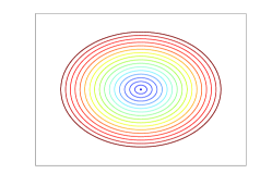
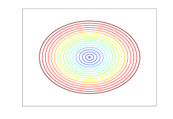
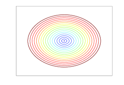
Figure 1: Contour plots: (i) Left: True solution, (ii) Center: Schrödinger, and (iii) Right: Fast sweeping

5.4.2 Comparison with the fast sweeping

In order to verify the accuracy of our technique, we compared our solution with fast sweeping for the following set of examples, using the latter as the ground truth as the true solution is not available in closed-form.

Example 2: In this example we solved the eikonal equation from a point source located at $(x_{0},y_{0})=(0,0)$ for the following forcing function

$$f(x,y)=1+2(e^{-2((x+0.05)^{2}+(y+0.05)^{2})}-e^{-2((x-0.05)^{2}+(y-0.05)^{2})})$$ (5.25)

on a $2D$ grid consisting of points between $(-0.125,-0.125)$ and $(0.125,0.125)$ with a grid width of $\frac{1}{2^{10}}$. We ran our method for $6$ iterations with $\hbar$ set at $0.015$ and fast sweeping for $15$ iterations sufficient for both techniques to converge. When we calculated the percentage error for the Schrödinger according to equation 5.24 (with fast sweeping as the ground truth), the error was just around $1.245\%$. The percentage error and maximum difference between the fast sweeping and Schrödinger solutions after each iteration are adumbrated in Table (3).

Table 3: Percentage error for the Schrödinger method in comparison to fast sweeping.

Iter	$\%error$	max diff
1	1.144632	0.008694
2	1.269028	0.008274
3	1.223836	0.005799
4	1.246392	0.006560
5	1.244885	0.006365
6	1.245999	0.006413

We believe that the fluctuations both in the percentage error and the maximum difference are due to repeated approximations of the integration involved in the convolution with discrete convolution and summation, but nevertheless stabilized after 6 iterations. The contour plots shown in Figure 2 clearly demonstrate the similarities between these methods.

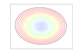
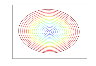
Figure 2: Contour plots: (i) Left: Schrödinger, (ii) Right: Fast sweeping

Example 3: Here we solved the eikonal equation for the sinusoidal forcing function

$$f(x,y)=1+\sin(\pi(x-0.05))\sin(\pi(y+0.05))$$ (5.26)

on the same $2D$ grid as in the previous example. We randomly chose $4$ grid locations namely,

$\{0,0\},\{0.0488,0.0977\},\{-0.0244,-0.0732\},\{0.0293,-0.0391\}$

as data locations and ran our method for $6$ iterations with $\hbar$ set at $0.0085$ and ran fast sweeping for $15$ iterations. The percentage error between the Schrödinger solution (after 6 iterations) and fast sweeping was $4.537\%$ with the maximum absolute difference between them being $0.0109$.

The contour plots are shown in Figure (3). Notice that the Schrödinger contours are more smoother in comparison to the fast sweeping contours.

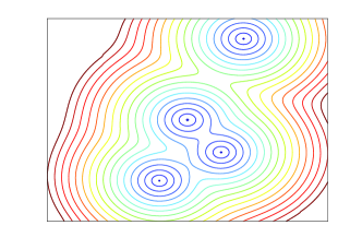
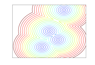
Figure 3: Contour plots: (i) Left: Schrödinger, (ii) Right: Fast sweeping

Example 4: Here we compared with fast sweeping on a larger $2D$ grid consisting of points between $(-5,-5)$ and $(5,5)$ with a grid width of $0.25$. We again considered the sinusoidal forcing function

$$f(x,y)=1+0.3\sin(\pi(x+1))\sin(\pi(y-2))$$ (5.27)

and chose 4 grid locations namely $\{0,0\},\{1,1\},\{-2,-3\},\{3,-4\}$ as data locations. Notice that the Green’s function $G$ and $\tilde{G}$ goes to zero exponentially faster for grid locations away from zero for small values of $\hbar$. Hence for a grid location say $(-4,4)$ which is reasonably far away from 0, the value of the Green’s function say at $\hbar=0.001$ may be zero even when we use a large number of precision bits $p$. This problem can be easily circumvented by first scaling down the entire grid by a factor $\tau$, computing the solution $S^{\ast}$ on the smaller denser grid and then rescaling it back again by $\tau$ to obtain the actual solution. It is worth emphasizing that scaling down the grid is tantamount to scaling down the forcing function as clearly seen from the fast sweeping method. In fast sweeping Zhao05 , the solution $S^{\ast}$ is computed using the quantity $f_{i,j}\delta$ where $f_{i,j}$ is the value of forcing function at the $(i,j)^{th}$ grid location and $\delta$ is the grid width. Hence scaling down $\delta$ by a factor of $\tau$ is equivalent to fixing $\delta$ and scaling down $f$ by $\tau$. Since the eikonal equation (1.1) is linear in $f$, computing the solution for a scaled down $f$–equivalent to a scaled down grid–and then rescaling it back again is guaranteed to give the actual solution.

The factor $\tau$ can be set to any desired quantity. For the current experiment we set $\tau=100$, $\hbar=0.001$ and ran our method for 6 iterations. Fast sweeping was run for 15 iterations. The percentage error between these methods was about $3.165\%$. The contour plots are shown in Figure 4. Again, the contours obtained from the Schrödinger are more smoother than those obtained from fast sweeping.

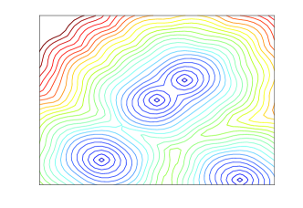
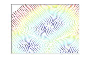
Figure 4: Contour plots: (i) Left: Schrödinger, (ii) Right: Fast sweeping

6 Discretization approach to solve the linear system with applications to path planning and shape from shading

As seen above, the perturbation technique requires repeated convolution of the Green’s function $G$ with the solution from the previous iteration $\phi_{i-1}$. As this convolution does not carry a closed form solution in general, we approximate the continuous convolution by its discrete counterpart computed via FFT. The error incurred from this discrete approximation tends to pile up with iteration. To circumvent this issue, a possible direct route to solving the screened Poisson equation in (4.1) is by discretization of the linear operator ($\nabla^{2}$) on a standard grid where the Laplacian is approximated by standard finite differences. Solving the discretized screened Poisson equation is far less complicated to implement than the fast marching or fast sweeping methods needed for directly solving (1.1). In addition, the computational complexity for implementing (4.1) can match these algorithms since $O(N)$ sparse, linear system solvers are available Saad03 . This comes from the fact that a finite difference approximation to (4.1), using a standard five-point Laplacian stencil, simply results in a sparse linear system of the form Demmel97 :

$$\underbrace{\left[\begin{array}[]{cccc}L_{N}+2I_{N}&-I_{N}&\cdots&0\\ -I_{N}&\ddots&\ddots&\vdots\\ \vdots&\ddots&\ddots&-I_{N}\\ 0&&-I_{N}&L_{N}+2I_{N}\end{array}\right]+\begin{bmatrix}f(X_{1})&0&\cdots&0\\ 0&f(X_{2})&\cdots&0\\ \vdots&\vdots&\ddots&\vdots\\ 0&0&\cdots&f(X_{N})\\ \end{bmatrix}}_{A}\underbrace{\left[\begin{array}[]{c}\phi_{1}\\ \phi_{2}\\ \vdots\\ \phi_{N}\end{array}\right]}_{x}=\underbrace{\left[\begin{array}[]{c}\delta_{kron}({\mathbf{x}}_{1})\\ \vdots\\ \delta_{kron}({\mathbf{x}}_{0})\\ \vdots\\ \delta_{kron}({\mathbf{x}}_{N})\end{array}\right]}_{b}$$ (6.14)

where $N$ represents the number of grid points and $L_{N}$ is a tri-diagonal block of the form

$$L_{N}=\left[\begin{array}[]{cccc}2&-1&&0\\ -1&\ddots&\ddots\\ &\ddots&\ddots&-1\\ 0&&-1&2\end{array}\right].$$

The function $\delta_{kron}({\mathbf{x}})$ in (LABEL:eq:sparse-system) is defined in (5.23) which is supported and takes the value one only at the point-set locations $\{{\mathbf{y}}_{k}\}_{k=1}^{K}$. Though better complexities are achievable using multigrid Saad03 solvers, one can just as well address many problems in a satisfactory manner using direct, sparse solvers, like MATLAB’s $A\backslash b$—an approach we adopt for the experiments in the present paper.

6.1 Path planning

In the pioneering contribution of Kimmel01 , Kimmel and Sethian developed one of the earliest applications of the eikonal equation to path planning. By finding a solution $S^{\ast}({\mathbf{x}})$ (referred to as the value function in the path planning context) to the eikonal equation in (1.1), we immediately recover the minimum cost to go from a source location ${\mathbf{x}}_{0}$ in the state space to any other point ${\mathbf{x}}$ (in the state space). Here, we impose the boundary condition $S^{\ast}({\mathbf{x}}_{0})=0$, and consider $f({\mathbf{x}})$ as the cost to travel through location ${\mathbf{x}}$ (higher the value, the more costly) and prescribe it as a strictly positive function. The function $f({\mathbf{x}})$ function is set to high values for undesirable travel regions for the optimal path, and very small values for favorable travel areas (and set to one on the source point). In comparison to other popular path planning techniques like potential field methods Khatib86 , the value function is an example of a navigation function—a potential field free of local minima.

Given a scalar field solution, the optimal paths are determined by gradient descent on $S^{\ast}({\mathbf{x}})$, and is typically referred to as backtracking. The backtracking procedure can be formulated as an ordinary differential equation

$$\dot{{\mathbf{x}}}=-\frac{\nabla S^{\ast}({\mathbf{x}}(t))}{\|\nabla S^{\ast}({\mathbf{x}}(t))\|},$$ (6.16)

whose solution ${\mathbf{x}}(t)$ is the reconstructed path from a fixed target location $\hat{{\mathbf{x}}}$. We typically terminate the gradient backtracking procedure at some $t$ value such that $\left\|{\mathbf{x}}(t)-{\mathbf{x}}_{0}\right\|$ $<\epsilon$, i.e. we get arbitrarily close the source point, for some small $\epsilon>0$. By construction, the backtracking on $S^{\ast}({\mathbf{x}})$ cannot get stuck in local minima—an obvious proof by contradiction validates this claim if one considers $S^{\ast}$ to be differentiable and have local minima $\nabla S^{\ast}=0$ at some ${\mathbf{x}}$, but $f({\mathbf{x}})>0$, and contradicts the eikonal equation $\|\nabla S^{\ast}\|=f({\mathbf{x}})$. Although, in theory, $S^{\ast}({\mathbf{x}})$ can contain saddle points, but usually this is not an issue in practice.

6.2 Anecdotal verification of path planning on complex mazes and extensions to vessel segmentation

We applied our path planning approach to a variety of complex maze images. We explicitly chose the maze grid sizes to be much larger than the norm for recent publications that apply the eikonal equation for path planning; these typical sizes are usually smaller than $100\times 100$. An objective juxtaposition of contemporary fast sweeping and marching techniques, which require special discretization schemes, data structures, sweep orders, etc., versus our approach presented here, clearly illustrates the efficiency and simplicity of the later. Our framework reduces path planning (a.k.a. all-pairs, shortest path or geodesic processing) implementation to four straightforward steps:

1. Define $f({\mathbf{x}})$, which assigns a high cost to untraversable areas in the grid and low cost to traversable locations. In the experiments here, we simply let appropriately scaled versions of the maze images be $f({\mathbf{x}})$, with white pixels representing boundaries and black pixels the possible solution paths.

2. Select a source point on the grid and a small value for $\hbar$. The solution to (4.1) will simultaneously recover all shortest paths back to this source from any non-constrained region in the grid.

3. Use standard finite differencing techniques to evaluate (4.1). This leads to a sparse, block tri-diagonal system which can be solved by a multitude of linear system numerical packages. We simply use MATLAB’s ’\’ operator. Recover approximate solution to eikonal by letting $S^{\ast}({\mathbf{x}})=-\hbar\log\phi({\mathbf{x}})$.

4. Backtrack to find the shortest path from any allowable grid location to the source, i.e. use eq. (6.16) to perform standard backtracking on $S^{\ast}({\mathbf{x}})$ .

The grid sizes and execution times for several mazes are provided in Table 4.

Table 4: Maze grids sizes and time to solve sparse system for path planning. Our approach simply uses MATLAB’s ’\’ operator to solve the shortest path problem, avoiding complex nuances of discretization schemes and specialized data structures required for fast marching.

2D Grid Dims. (No. of Points)	$A\backslash b$ (sec.)
$450\times 450$ $\left(N=202,500\right)$, Fig. 5	0.79
$434\times 493$ $\left(N=213,962\right)$, Fig. 6(a)	1.02
$621\times 473$ $\left(N=293,733\right)$, Fig. 6(b)	1.22
$419\times 496$ $\left(N=207,824\right)$, Fig. 6(c)	0.77

Notice that even for larger grids, our time to solve for $S^{\ast}({\mathbf{x}})$ is on the order of a few seconds, and this is simply using the basic sparse solver in MATLAB. The time complexity of MATLAB’s direct solver is $O\left(N^{1.5}\right)$, which makes our approach here slightly slower than the optimal runtime. $O\left(N\right)$ is achievable for sparse systems, such as ours, using multigrid methods, but we have opted to showcase the simplicity of our implementation versus pure speed. Figure 5 illustrates the resulting optimal paths from three different locations.

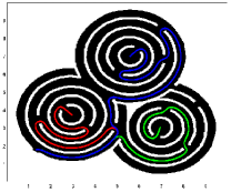
Figure 5: Optimal paths from various locations to common source. (Note: constraint areas are in white and traversable regions in black.)

Figure 6 illustrates our path planing approach on a variety of mazes: (a) demonstrates path planning while paying homage to Schrödinger’s cat, (b) is a traditional maze, and (c) is a whimsical result on a skull maze. Notice in all these mazes there are multiple solution paths back to the source, but only the shortest path is chosen.

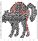
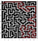
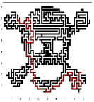
(a)	(b)	(c)

Figure 6: (a) Schrödinger’s cat maze, (b) standard maze, (c) skull maze. Multiple solutions are possible but only the shortest path is chosen to be optimal. (Note: constraint areas are in white and traversable regions in black.)

The above discussed application of path planning can be readily extended to centerline extraction from medical imagery of blood vessels. One can view the image $I({\mathbf{x}})$ as a “maze” where we only want to travel on the vessels in the image. Figure 7, column (a) illustrates three example medical images: eye, brain, and hand. Columns (b) showcases our results, while (c) provides comparative analysis against fast sweeping. Notice that our solution naturally generates smoother centerline segmentations, which is a natural consequence of having a built-in, viscosity-like term in (4.5). Whereas, the fast marching and fast sweeping methods tend to have sharper transitions in the paths and deviate from the center—viscosity solutions can be used to alleviate this, but are not organic to the formulation like ours. In fact, it has been shown that additional constraints have to be incorporated to ensure fast marching approaches extract the centerline Cohen2001 . Again, we stress the simplicity and ease-of-use of this approach, with only one free parameter $\hbar$, making it a viable option for many path planning related applications, such as robotic navigation, optimal manipulation, and vessel extraction in medical images.

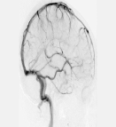
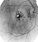
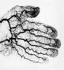
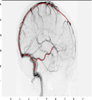
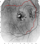
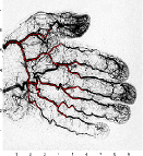
Figure 7: Medical image vessel centerline extraction, top row original images and bottom row our linear solution approach. Paths under our linear systems approach are smooth due to inherent viscosity-like behavior. They also produce segmentations where the extracted vessels are centered on the blood vessels. Fast marching approach requires additional constraints to achieve centerline extraction Cohen2001 .

6.3 Shape-from-Shading

Shape-from-shading has long been a popular problem domain for computer vision, having the primary objective of recovering the scalar height field from a single image. Solution approaches utilizing the eikonal equation have been known since the early 80’s Bruss82 , and have continually improved upon through the advent of fast sweeping and fast marching methods Kimmel01 ; Pardos06 . The standard forward image model assuming a Lambertian reflectance model generates the luminance via inner product of the surface normal, ${\mathbf{n}}({\mathbf{x}})$, with the light source direction, ${\mathbf{d}}$., i.e. $P({\mathbf{x}})=\langle{\mathbf{n}}({\mathbf{x}}),{\mathbf{d}}\rangle$. For example, if we assume a vertical lighting direction ${\mathbf{d}}=[0,\,0,\,1]^{T}$, we get the imaging operator

$$P({\mathbf{x}})=\frac{1}{\sqrt{\left\|\nabla S^{\ast}({\mathbf{x}})\right\|^{2}+1}},$$

where $S^{\ast}({\mathbf{x}})$ is the desired scalar height field we wish to recover. This can be obtained by solving the standard eikonal equation (1.1) with

$$f({\mathbf{x}})=\sqrt{\frac{1}{P({\mathbf{x}})^{2}}-1}$$ (6.17)

and boundary conditions $S^{\ast}({\mathbf{x}}_{i})=h_{i}$, i.e. we seed the boundary conditions with the known heights $h_{i}$ at select grid locations $X_{i}$.

As we have detailed in previous sections, our formalism allows one to address any general (non-linear) eikonal equation by solving the linear screened Poisson equation in (4.1). One simply needs to create the forcing function in (6.17) and then solve the discretized sparse system as in (LABEL:eq:sparse-system). This immediately yields the recovered height field.

6.4 Surface reconstruction via shape from shading

For shape from shading, we validated height recovery on two common images that often used in the literature: Mozart and a vase. Figure 8 illustrates the recovered surfaces using our method, (a), fast marching, (b), and fast sweeping, (c). Under each image we also list the error of the reconstruction from the known ground truth height field. The error was computed by comparing the true mean gradient magnitudes versus those estimated from the recovered $S^{\ast}({\mathbf{x}})$.

The validation shows that our method is competitive with both fast marching and fast sweeping, all the while retaining the efficiency and simplicity of obtain a solution through a sparse linear system. Going beyond the present work, our general framework can be adapted to all previous application areas of the eikonal equation, and, as alluded to earlier, the variational objective can be readily modified for to incorporate other constraints that may lead to better reconstructions.

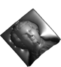
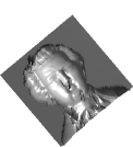
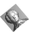
Error: 0.524438	Error: 0.713825	Error: 0.654674
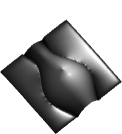
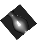
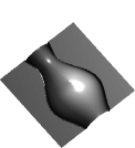
Error: 0.203321	Error: 0.237820	Error: 0.199234
(a)	(b)	(c)

Figure 8: Shape-from-shading surface reconstruction, per column: (a) our linear solution approach, (b) fast marching, (c) fast sweeping. Based on the gradient magnitude error (from the true surface), our approach linear systems approach is better or at least highly competitive.

7 Conclusion

The Hamilton-Jacobi equation, particularly its specialized form as the eikonal equation, is at the heart of numerous applications in vision (shape-from-shading, path planning, medial axis, etc.), and spurred the rapid development of several innovative computational techniques to directly solve this nonlinear PDE, including fast marching, and fast sweeping. However, lost in this flurry of advancing nonlinear solvers was a completely alternative approach, one which allows you to rigorously approximate solutions to the nonlinear eikonal as a limiting case of the solution to a corresponding linear Schrödinger equation. Instead of directly solving the eikonal equation, the Schrödinger formalism results in a generalized, screened Poisson equation which is solved at very small values of $\hbar$. In addition, a direct consequence of our mathematical formulation is that viscosity solutions are naturally incorporated and obtained when solving the linear differential equation—allowing one to circumvent explicit viscosity constructions required for any method that tries to directly solve the nonlinear eikonal.

We initially developed a fast and efficient perturbation series method for solving the generalized, screened Poisson equation which is guaranteed to converge provided the forcing function $f$ is positive and bounded. Using the perturbation method and the relation (4.6), we obtained the solution for the eikonal equation without spatially discretizing the operators. We later saw that the spatial discretization of the Laplacian operator resulted in a sparse, linear system using which we developed novel solutions to the classical all-pairs, shortest path problem (a.k.a. path planning). We also illustrated results on shape-from-shading and vessel centerline extraction. Our approach is straightforward to implement (by deploying any sparse linear solver) and holds its own against contemporary fast marching and fast sweeping methods while possessing the considerable advantage of linearity.

Our Schrödinger-based approach follows the pioneering Hamilton-Jacobi solvers such as the fast sweeping Zhao05 and fast marching Osher88 methods with the crucial difference being its linearity. In future work, we plan to revisit past uses of the eikonal equation and examine improvements gained by the adoption of our linear framework. We are also investigating extensions of this approach to other areas such as control theory.

References

- (1) M. Abramowitz and I. A. Stegun, Handbook of mathematical functions with formulas, graphs and mathematical tables, Dover, New York, NY, 1964.
- (2) V. I. Arnold, Mathematical methods of classical mechanics, Springer, New York, NY, 1989.
- (3) J. L. Basdevant, Variational principles in physics, Springer, New York, NY, 2007.
- (4) R. N. Bracewell, The Fourier transform and its applications, 3rd ed., McGraw-Hill, New York, NY, 1999.
- (5) A. R. Bruss, The eikonal equation: some results applicable to computer vision, J. Math. Phys. 23 (1982), no. 5, 890–896.
- (6) J. Butterfield, On Hamilton-Jacobi theory as a classical root of quantum theory, Quo-Vadis Quantum Mechanics, Springer, New York, NY, 2005, pp. 239–274.
- (7) J. F. Canny, Complexity of robot motion planning, The MIT Press, Cambridge, MA, 1988.
- (8) G. Chartier, Introduction to optics, Springer, New York, NY, 2005.
- (9) J. W. Cooley and J. W. Tukey, An algorithm for the machine calculation of complex Fourier series, Math. Comp. 19 (1965), no. 90, 297–301.
- (10) T. H. Cormen, C. E. Leiserson, R. L. Rivest, and C. Stein, Introduction to algorithms, 2nd ed., The MIT Press, Cambridge, MA, September 2001.
- (11) M. G. Crandall, H. Ishii, and P.L. Lions, User’s guide to viscosity solutions of second order partial differential equations, Bulletin of the American Mathematical Society 27 (1992), no. 1, 1–67.
- (12) J. W. Demmel, Applied numerical linear algebra, SIAM, 1997.
- (13) T. Deschamps and L. D. Cohen, Fast extraction of minimal paths in 3D images and applications to virtual endoscopy, Med. Image Anal. 5 (2001), no. 4, 281–299.
- (14) F. M. Fernandez, Introduction to perturbation theory in quantum mechanics, CRC press, 2000.
- (15) A. L. Fetter and J. D. Walecka, Theoretical mechanics of particles and continua, Dover, New York, NY, 2003.
- (16) L. Fousse, G. Hanrot, V. Lefévre, P. Pélissier, and P. Zimmermann, MPFR: A multiple-precision binary floating-point library with correct rounding, ACM Trans. Math. Softw. 33 (2007), 1–15.
- (17) H. Goldstein, C.P. Poole, and J. L. Safko, Classical mechanics, 3rd ed., Addison Wesley, Boston, MA, 2001.
- (18) T. Granlund and et al., GNU MP: The GNU Multiple Precision Arithmetic Library, 2012, url:http://gmplib.org/.
- (19) D. J. Griffiths, Introduction to quantum mechanics, 2nd ed., Prentice Hall, Upper Saddle River, NJ, 2005.
- (20) K. S. Gurumoorthy and A. Rangarajan, A Schrödinger equation for the fast computation of approximate Euclidean distance functions, SSVM, LNCS, vol. 5567, Springer, 2009, pp. 100–111.
- (21) O. Khatib, Real-time obstacle avoidance for manipulators and mobile robots, Int. J. Robot. Res. 5 (1986), no. 1, 90–98.
- (22) R. Kimmel and J. A. Sethian, Optimal algorithm for shape from shading and path planning, J. Math. Imaging Vision 14 (2001), 237–244.
- (23) R.G. Newton, Scattering Theory of Waves and Particles, 2nd ed., Springer-Verlag, New York, 1982.
- (24) S. J. Osher and R. P. Fedkiw, Level set methods and dynamic implicit surfaces, Springer-Verlag, New York, NY, October 2003.
- (25) S. J. Osher and J. A. Sethian, Fronts propagating with curvature dependent speed: Algorithms based on Hamilton-Jacobi formulations, J. Comp. Phys. 79 (1988), no. 1, 12–49.
- (26) E. Pardos and O. Faugeras, Handbook of mathematical models in computer vision, ch. Shape from Shading, pp. 275–388, Springer, 2006.
- (27) D.T. Paris and F.K. Hurd, Basic Electromagnetic Theory, McGraw-Hill Education, 1969.
- (28) Y. Saad, Iterative methods for sparse linear systems, 2nd ed., SIAM, 2003.
- (29) M. Sethi, A. Rangarajan, and K. S. Gurumoorthy, The Schrödinger Distance Transform (SDT) for point-sets and curves, CVPR, IEEE Computer Society, 2012, pp. 198–205.
- (30) J. A. Sethian, A fast marching level set method for monotonically advancing fronts, Proc. Nat. Acad. Sci. 93 (1996), no. 4, 1591–1595.
- (31) G. B. Whitham, Linear and nonlinear waves, Pure and Applied Mathematics, Wiley-Interscience, 1999.
- (32) L. Yatziv, A. Bartesaghi, and G. Sapiro, O(N) implementation of the fast marching algorithm, J. Comp. Phys. 212 (2006), no. 2, 393–399.
- (33) H. K. Zhao, A fast sweeping method for eikonal equations, Math. Comp. 74 (2005), no. 250, 603–627.