The multi-scale environment of RS Cnc from CO and H i observations

We present a detailed study of the circumstellar gas distribution and kinematics of the semi-regular variable star RS Cnc on spatial scales ranging from $\sim 1^{\prime\prime}$ ($\sim$150 AU) to $\sim 6^{\prime}$ ($\sim$0.25 pc). Our study utilizes new CO1-0 data from the Plateau-de-Bure Interferometer and new H i 21-cm line observations from the Jansky Very Large Array (JVLA), in combination with previous observations. New modeling of CO1-0 and CO2-1 imaging observations leads to a revised characterization of RS Cnc’s previously identified axisymmetric molecular outflow. Rather than a simple disk-outflow picture, we find that a gradient in velocity as a function of latitude is needed to fit the spatially resolved spectra, and in our preferred model, the density and the velocity vary smoothly from the equatorial plane to the polar axis. In terms of density, the source appears quasi-spherical, whereas in terms of velocity the source is axi-symmetric with a low expansion velocity in the equatorial plane and faster outflows in the polar directions. The flux of matter is also larger in the polar directions than in the equatorial plane. An implication of our model is that the stellar wind is still accelerated at radii larger than a few hundred AU, well beyond the radius where the terminal velocity is thought to be reached in an asymptotic giant branch star. The JVLA H i data show the previously detected head-tail morphology, but also supply additional detail about the atomic gas distribution and kinematics. We confirm that the ‘head’ seen in H i is elongated in a direction consistent with the polar axis of the molecular outflow, suggesting that we are tracing an extension of the molecular outflow well beyond the molecular dissociation radius (up to $\sim$0.05 pc). The $6^{\prime}$-long H i ‘tail’ is oriented at a PA of 305^∘, consistent with the space motion of the star. The tail is resolved into several clumps that may result from hydrodynamic effects linked to the interaction with the local interstellar medium. We measure a total mass of atomic hydrogen $M_{\rm HI}\approx 0.0055M_{\odot}$ and estimate a lower limit to the timescale for the formation of the tail to be $\sim 6.4\times 10^{4}$ years.

1 Introduction

Asymptotic Giant Branch (AGB) stars are undergoing mass loss at a high rate. One of the best tracers of AGB outflows are the rotational lines of carbon monoxide (CO). From the modeling of the line profiles it has been possible to derive reliable expansion velocities and mass loss rates (Ramstedt et al. 2008). In addition imaging at high spatial resolution allows us to describe the geometry and the kinematics of these outflows in the inner circumstellar regions where the winds emerge and where their main characteristics get established (Neri et al. 1998).

High quality observations of CO line emissions at high spectral resolution have shown that some profiles are composite, with a narrow component superimposed on a broader one, revealing the presence of two winds with different expansion velocities (Knapp et al. 1998, Winters et al. 2003). Using high spatial resolution data obtained in the CO1-0 and 2-1 lines, Libert et al. (2010) have suggested that the composite line-profiles of the semi-regular AGB star RS Cnc probably originate from an axi-symmetrical geometry with a slowly expanding equatorial disk and a faster perpendicular bipolar outflow. Other cases of AGB stars with axi-symmetrical expanding shells have been identified in a CO mapping survey of AGB stars by Castro-Carrizo et al. (2010). It shows that the axi-symmetry which is often observed in post-AGB stars (e.g. Sahai et al. 2007) may develop earlier when the stars are still on the AGB.

Although extremely useful, CO as a tracer is limited to the inner parts of the circumstellar shells because, at a distance of typically $\sim$ 10¹⁷ cm, it is photo-dissociated by the interstellar radiation field (ISRF). At larger distances, it is necessary to use other tracers, such as dust or atomic species. The H i line at 21 cm has proved to be an excellent spatio-kinematic tracer of the external regions of circumstellar shells (e.g. Gérard & Le Bertre 2006, Matthews & Reid 2007). In particular, the H i map of RS Cnc presented by Matthews & Reid shows a 6^′-long tail, in a direction opposite to the space motion of the central star, and clearly different from that of the bipolar flow observed in CO at shorter distances (2–10^′′) by Libert et al. (2010). In such a case the shaping mechanism is thought to be due to the motion of the star relative to the local interstellar medium (Libert et al. 2008, Matthews et al. 2013).

Thus RS Cnc is an ideal target to study, in the same source, the two main effects that are expected to shape circumstellar environments, and to evaluate their respective roles. In this paper, we revisit RS Cnc with new high spatial resolution data obtained in CO at 2.6 mm and in H i at 21 cm. Our goal is to combine observations in these two complementary tracers, in order to describe the spatio-kinematic structure of the circumstellar shell from its center to the interstellar medium (ISM). The stellar properties of RS Cnc are summarized in Table 1.

Until recently, a distance of 122 pc was adopted from the parallax measured using Hipparcos (Perryman et al. 1997). However, new analyses of the Hipparcos data led to somewhat larger estimates of the distance, 129${}_{-16}^{+16}$ pc (Famaey et al. 2005) and 143${}_{-10}^{+12}$  pc (van Leeuwen 2007). In the present work, we adopt the improved values of the parallax and proper motions by van Leeuwen, and scale the published results with the new estimate of the distance. We also adopt the peculiar solar motion from Schönrich et al. (2010). RS Cnc is an S-type star (CSS 589, in Stephenson’s (1984) catalogue) in the Thermally-Pulsing AGB phase of evolution: Lebzelter & Hron (1999) reported the presence of Tc lines in its spectrum.

Table 1: Properties of RS Cnc.

parameter	value	ref.
distance	143 pc	1
MK Spectral type	M6eIb-II(S)	2
variability type	SRc:	2
pulsation periods	122 and 248 days	3
effective temperature	3226 K	4
radius	225 R⊙	4
luminosity	4945 L⊙	4
LSR radial velocity (V⋆)	6.75 km s-1	5
expansion velocity	2.4/8.0 km s-1	5
mass loss rate	1.7 10-7 M⊙ yr-1	6
3D space velocity; PA	15 km s-1; 155∘	this work

References in the table:
(1) Hipparcos (van Leeuwen 2007)
(2) GCVS (General Catalogue of Variable Stars)
(3) Adelman & Dennis (2005)
(4) Dumm & Schild (1998)
(5) Libert et al. (2010)
(6) Knapp et al. (1998)

2 CO observations

2.1 summary of previous data

RS Cnc was imaged in the CO1-0 and 2-1 lines by Libert et al. (2010). An on-the-fly (OTF) map covering a region of 100${}^{\prime\prime}\times$100^′′ with steps of 4^′′ in RA and 5^′′ in Dec was obtained at the IRAM 30-m telescope. Interferometric data were obtained with the Plateau-de-Bure Interferometer (PdBI) in three configurations, B, C and D, i.e. with baselines ranging from 24-m to 330-m. All sets of observations were obtained with a spectral resolution corresponding to 0.1 km s^-1. The data from the 30-m telescope and the PdBI were merged and images in 1-0, with a field of view (fov) of 44^′′ and a spatial resolution of $\sim$2.3^′′, and in 2-1, with a fov of 22^′′ and a spatial resolution of $\sim$1.2^′′, were produced. Libert et al. presented the corresponding channel maps with a spectral resolution of 0.4 km s^-1.

These maps show clearly that the broad and narrow spectral components reported by Knapp et al. (1998) originate from two different regions that Libert et al. (2010) described as a slowly expanding ($\sim$ 2 km s^-1) equatorial disk/waist and a faster ($\sim$ 8 km s^-1) bipolar outflow. Libert et al. estimated that the polar axis lies at an inclination of $\sim 45^{\circ}$ with respect to the plane of the sky and is projected almost north-south, along a position angle (PA) of $\sim 10^{\circ}$.

2.2 new data

In January and February 2011, we obtained new data in the CO1-0 line with the PdBI array in configurations A and B, increasing the baseline coverage up to 760 m.

The new data were obtained in dual polarizations and covered a bandwidth of 3.6 GHz centered at 115.271 GHz, the nominal frequency of the CO1-0 line. Two units of the narrow band correlator were set up to cover the CO line with a spectral resolution of 39 kHz over a bandwidth of 20 MHz, and the adjacent continuum was observed by the wideband correlator WideX (Wideband Express) with a channel spacing of 1.95 MHz.

These observations resulted in 12 h of on-source integration time with the 6 element array and reach a 1$\sigma$ thermal noise level of 12 mJy/beam in 0.2 km s^-1 channels. The synthesized beam is 0.92${}^{\prime\prime}\times$ 0.78^′′ at a position angle PA$=62^{\circ}$.

2.3 continuum

We used the new WideX data to produce a continuum image of RS Cnc at 115 GHz. The data were integrated over a 2 GHz band, excluding the high frequency portion of the band that is affected by atmospheric absorption. A single point source is clearly detected. The source is unresolved, and there is no evidence of a companion. It has a flux density of 5.4$\pm$0.3 mJy, which is consistent with the flux density reported by Libert et al. (2010). It is slightly offset south-west with respect to the center of phase because we used the coordinates at epoch 2000.0 from Hipparcos. The offset (–0.15^′′ in RA and –0.37^′′ in Dec) is consistent with the proper motion reported by Hipparcos ($-$11.12 mas yr^-1 in RA and –33.42 mas yr^-1 in Dec, van Leeuwen 2007).

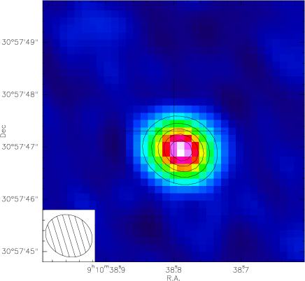
Figure 1: Continuum map at 115 GHz of RS Cnc (A+B configuration data obtained in 2011). The cross corresponds to the 2000.0 position of the star (RA 09:10:38.800, Dec 30:57:47.30). The contour levels are separated by steps of 0.90mJy/beam ($\equiv$ 20$\sigma$). The beam is 0.92${}^{\prime\prime}\times 0.78^{\prime\prime}$ (PA = 62^∘).

2.4 channel maps in CO1-0

The channel maps obtained in 2011 across the CO1-0 line are dominated by a compact central source. However, at 6.6 km s^-1 (Fig. 2), we observe a companion source at $\sim$1^′′ west-north-west (PA$\sim$300^∘). This source is detected from 5.8 to 6.8 km s^-1, but not outside this range. In the channel map at 6.6 km s^-1, in which it is best separated, it has an integrated flux of 93$\pm$6 mJy, as compared to 300$\pm$20 mJy for the central source. This secondary source is clearly not at the origin of the bipolar outflow, which is aligned on the central source. Within errors, the central source coincides with the continuum source discussed in the previous section.

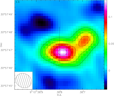
Figure 2: Continuum subtracted CO1-0 channel map at 6.6 km s^-1 (A+B configuration data obtained in 2011). The contour levels are separated by steps of 24 mJy/beam ($\equiv\,2\sigma$). The negative contours are in dotted lines.

2.5 merging (CO1-0)

Finally, the new data (observed in the extended A and B configurations) were merged with the old ones already presented by Libert et al. (2010). These were obtained in the previous B, C, and D configurations and combined with short spacing observations obtained on the IRAM 30 m telescope. The final combined data set now covers a spectral bandwidth of 580 MHz, resampled to a spectral resolution of 0.2 km s^-1. The 1 $\sigma$ thermal noise in the combined data cube is 8.7 mJy/beam (for a channel width of 0.2 km s^-1) and the synthesized beam is 1.15${}^{\prime\prime}\,\times$0.96^′′ at PA = 67^∘, similar to the resolution already obtained on CO2-1 (Libert et al. 2010).

In Fig. 3, we present the resulting spectral map that we have derived by using a circular restoring beam with a gaussian profile of FWHM = 1.2^′′. The line profiles are composed of three components whose relative intensities depend on the position in the map. One notes also that the two extreme components, at $\sim$ 2 km s^-1 and $\sim$12 km s^-1, tend to deviate more from the central component as the distance to the central source increases. In Fig. 4, three spectra obtained in the south of the central position are overlaid. One notes a shift in velocity of the red peaks, which correspond to the southern polar outflow at $\sim$12-14 km s^-1) relative to the central peaks at $\sim$5-8 km s^-1, which correspond to the emission close to the equatorial plane, with distance to the central source.

Figure 3: CO1-0 spectral map of RS Cnc obtained with a restoring beam of 1.2^′′. The offsets with respect to the center of phase are given in the upper left corner of each panel (step=1.4^′′). North is up, and east is to the left.

Figure 4: Spectra obtained at different positions (centre, 1.4^′′ south, 2.8^′′ south) in a beam of 1.2^′′ (cf. Fig. 3).

3 CO model

3.1 description

In order to constrain the spatio-kinematic structure of RS Cnc, we have constructed a model of CO emission adapted to any geometry and based on a code already developed by Gardan et al. (2006). A ray-tracing approach, taking into account the velocity-dependent emission and absorption of each element along a line of sight, allows us to reconstruct the flux obtained, within an arbitrary beam, from a source which has an arbitrary geometry. The density, the excitation temperature and the velocity are defined at each point of the circumstellar shell. The code can then produce synthetic spectral maps that can be compared to the observed ones.

The populations of the rotational levels of the CO molecules are calculated assuming local thermodynamic equilibrium. The temperature profile is assumed to vary as r^-0.7, where r is the distance from the center of the star, and is scaled to models kindly provided by Schöier & Olofsson (2010, private communication; Fig. 5). The latter profiles were obtained using the radiative transfer code developed in spherical geometry by Schöier & Olofsson (2001). The same temperatures are adopted to calculate for each element the thermal Doppler broadening, assuming a Maxwellian distribution of the velocities.

Figure 5: Temperature profiles for different mass loss rates from Schöier & Olofsson (2010, private communication). The thin line represents the temperature profile adopted in this work.

3.2 application to RS Cnc

Following Libert et al. (2010) the source is defined by an equatorial plane and a polar axis. It is thus axi-symmetric and we need only two angles, which for instance define the orientation of the polar axis. Hereby, for simplicity we will use the angle of inclination of this axis over the plane of the sky (AI), and the position angle of the projection on the plane of the sky of this axis of symmetry (PA).

We assume that the velocities are radial and that the outflows are stationary. Thus, the product v$\times$n$\times$r² (where v is the velocity, n the density, and r the distance to the centre) is kept constant along every radial direction. In order to account for the velocity gradient observed in the line profiles (Fig. 4), we adopt a dependence of the velocity in r^α, $\alpha$ being the logarithmic velocity gradient (Nguyen-Q-Rieu et al. 1979).

We adopt a stellar CO/H abundance ratio of 4.0 10^-4 (all carbon in CO, Smith & Lambert 1986). Then we take a dependence of the CO abundance ratio with r from the photo-dissociation model of Mamon et al. (1988) for a mass loss rate of 1.0$\times 10^{-7}$ M_⊙ yr^-1 (see below). The external limit is set at 20^′′ ($\sim$ 4.3 10¹⁶ cm). In addition, we assume an He/H abundance ratio of 1/9. The star is offset from the center of the map by the amount measured on the continuum map (Fig. 1). Finally, we adopt a stellar radial velocity V_lsr = 6.75 km s^-1 (cf. Table 1).

In our preferred model of RS Cnc, the density and the velocity are varying smoothly from the equatorial plane to the polar axis. The profiles of the density and the velocity are shown in Figs. 6 and 7, respectively. The latitude ($\theta$, $\mu$=sin$\theta$) dependence was obtained by a combination of exponential functions of $\mu$. In order to adjust the parameters of the model we used the minuit package from the CERN program library (James & Roos 1975), which minimizes the sum of the square of the deviations (i.e. modeled minus observed intensities). The minimization is obtained on the CO1-0 spectral map, which has the best quality, and the same parameters are applied for the CO2-1 map. The flux of matter varies from 0.53$\times 10^{-8}$ M_⊙ yr^-1 sr^-1 in the equatorial plane to 1.59$\times 10^{-8}$ M_⊙ yr^-1 sr^-1 in the polar directions (Fig. 8). The total mass loss rate is 1.24$\times 10^{-7}$ M_⊙ yr^-1. The mass loss rate integrated within the two polar cones ($|\mu|>$0.5) is 0.83$\times 10^{-7}$ M_⊙ yr^-1. The exponent in the velocity profile varies from $\alpha$ = 0.13 in the equatorial plane, to $\alpha$ = 0.16 in the polar directions (Fig. 9).

Figure 6: The density profiles (in hydrogen atom number) in our preferred model as a function of $\mu$ ($\equiv$ sin $\theta$, $\theta$ being the angle with respect to the equator) and for various distances from the central star. The profile for r=1 arcsec (r= 0.1 arcsec) is scaled by a factor 1/100 (1/10000, respectively).

Figure 7: Same as in Fig. 6, but for the velocity.

Figure 8: The flux of matter as a function of $\mu$.

Figure 9: Velocity profiles in the equatorial plane ($\mu$ = 0) and along the polar axis ($\mu=\pm$ 1).

In Figs. 10 and 11, we present a comparison of the spectra obtained in CO1-0 and CO2-1 together with the results of the model. We obtain a good compromise between the 2-1 and 1-0 data and the model, although with a slight excess of the model in 2-1 in particular in the central part of the map. The orientation of the source obtained with the minimization algorithm is defined by AI = 52^∘ (angle of inclination of the polar axis over the plane of the sky), and PA = 10^∘ (position angle of the projection of this axis over the plane of the sky).

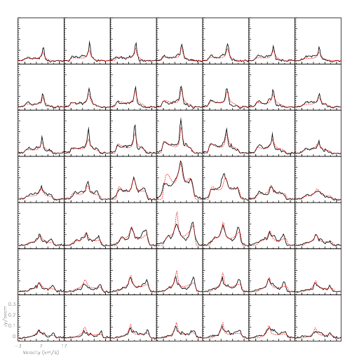
Figure 10: Central part of the CO1-0 spectral map of RS Cnc together with the fits (dotted lines, in red in the electronic version) obtained in Sect. 3.2.

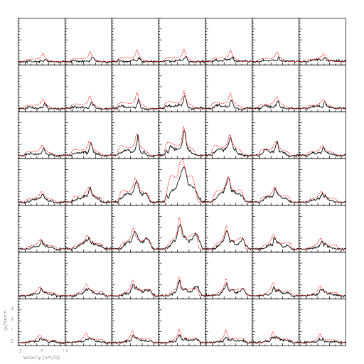
Figure 11: Same as in Fig. 10, but for CO2-1. The original Libert et al. (2010) data have been resampled to 0.2 km s^-1.

4 VLA and JVLA Observations

H i imaging observations of RS Cnc obtained with the Very Large Array (VLA) in its D configuration (0.035-1.03 km baselines) were previously presented by Matthews & Reid (2007; see also Libert et al. 2010). Those data were acquired using dual circular polarizations and a 0.77 MHz bandpass. On-line Hanning smoothing was applied in the VLA correlator, yielding a data set with 127 spectral channels and a channel spacing of 6.1 kHz ($\sim$1.29 km s^-1). Further details can be found in Matthews & Reid.

For the present analysis, the VLA D configuration data were combined with new H i 21-cm line observations of RS Cnc obtained using the Jansky Very Large Array (JVLA; Perley et al. 2011) in its C configuration (0.035-3.4 km baselines). The motivation for the new observations was to obtain information on the structure and kinematics of the H i emission on finer spatial scales than afforded by the D configuration data alone, thereby enabling a more detailed comparison between the H i and CO emission (see Sect. 2).

The JVLA C configuration observations of RS Cnc were obtained during observing sessions on 2012 March 2 and 2012 April 19. A total of 4.8 hours was spent on-source. Observations of RS Cnc were interspersed with observations of the phase calibrator J0854+2006 approximately every 20 minutes. 3C286 (1331+305) was observed as a bandpass and absolute flux calibrator.

The JVLA WIDAR correlator was configured with 8 subbands across each of two independent basebands, both of which measured dual circular polarizations. Only data from the first baseband pair (A0/C0) were used for the present analysis. Each subband had a bandwidth of 0.25 MHz with 128 spectral channels, providing a channel spacing of 1.95 kHz ($\sim$0.41 km s^-1). The 8 subbands were tuned to contiguously cover a total bandwidth of 2 MHz.

The bulk of the JVLA data were taken with the central baseband frequency slightly offset from the LSR velocity of the star. However, additional observations of the phase and bandpass calibrators were made with the frequency center shifted by $-1.5$ MHz and $+$1.5 MHz, respectively, to eliminate contamination from Galactic H i emission in the band and thus permit a robust bandpass calibration and more accurate bootstrapping of the flux density scale.

Data processing was performed using the Astronomical Image Processing System (AIPS; Greisen 2003). Data were loaded into AIPS directly from archival science data model (ASDM) format files using the BDFIn program available in the Obit software package (Cotton 2008). This permitted the creation of tables containing on-line flags and system power measurements.

After updating the antenna positions and flagging corrupted data, an initial calibration of the visibility data was performed using the AIPS task TYAPL, which makes use of the system power measurements to provide optimized data weights (Perley 2010). Calibration of the bandpass and the frequency-independent portion of the complex gains was subsequently performed using standard techniques, taking into account the special considerations for JVLA data detailed in Appendix E of the AIPS Cookbook. The gain solutions for the fifth subband were interpolated from the adjacent subbands because of line contamination. Following these steps, time-dependent frequency shifts were applied to the data to compensate for the Earth’s motion.

Figure 12: H i channel images of RS Cnc obtained from combined (J)VLA C and D configuration data. Contour levels are ($-$6[absent],$-$4.2,$-$3,3,4.2,6,8.5)$\times$1.4 mJy beam^-1. A $u$-$v$ tapering of 4k$\lambda$ (see Sect. 4.2) was used to produce these images. The lowest contour is $\sim 3\sigma$. The synthesized beam size is $57^{\prime\prime}\,.9$$\times$$54^{\prime\prime}\,.2$. The star symbol marks the stellar position of RS Cnc from Hipparcos.

4.1 Imaging the Continuum

An image of the 21-cm continuum emission within a $\sim 50^{\prime}$ region centered on the position of RS Cnc was produced using only the C configuration data. After excluding the first and last two channels of each subband and the portion of the band containing line emission, the effective bandwidth was $\sim$1.7 MHz in two polarizations.

Robust +1 weighting (as implemented in AIPS) was used to create the continuum image, producing a synthesized beam of $17^{\prime\prime}\,.4$$\times$$14^{\prime\prime}\,.3$. The RMS noise in the resulting image was $\sim$ 0.11 mJy beam^-1.

The brightest continuum source within the $\sim 30^{\prime}$ JVLA primary beam was located $\sim$$12^{\prime}\,.6$ northwest of RS Cnc, with a flux density of 110$\pm$1 mJy. No continuum emission was detected from RS Cnc itself, and we place a 3$\sigma$ upper limit on the 21 cm continuum emission at the position of the star within a single synthesized beam to be $<$0.33 mJy. Using Gaussian fits, we compared the measured flux densities of the six brightest sources in the primary beam with those measured from NRAO VLA Sky Survey (Condon et al. 1998), and found the respective flux densities to be consistent to within formal measurement uncertainties.

4.2 Imaging the H i Line Emission

Because the C and D configuration observations of RS Cnc were obtained with different spectral resolutions, prior to combining them the C configuration data were boxcar smoothed and then resampled to match the channel spacing of VLA D configuration data. Subsequently, the C and D configuration data sets were combined using weights that reflected their respective gridding weight sums as reported by the AIPS task IMAGR. The combined data set contained 127 spectral channels with a channel spacing of 6.1 kHz and spanned the LSR velocity range from $+81.2$ km s^-1 to $-$81.2 km s^-1. Before imaging the line emission, the continuum was subtracted from the combined data set using a first order fit to the real and imaginary parts of the visibilities in the line-free portions of the band (taken to be spectral channels 10-50 and 77-188).

Three different H i spectral line image cubes were produced for the present analysis. The first used natural weighting of the visibilities, resulting in a synthesized beam size of $36^{\prime\prime}\,.2$$\times$$31^{\prime\prime}\,.6$ at a position angle (PA) of $87^{\circ}$ and an RMS noise of $\sim$1.1 mJy beam^-1 per channel. For the second image cube, the visibility data were tapered using a Gaussian function with a width at the 30% level of 4 k$\lambda$ in the $u$ and $v$ directions. This resulted in a synthesized beam of $57^{\prime\prime}\,.9$$\times$$54^{\prime\prime}\,.1$ at PA=$-88^{\circ}$ and an RMS noise level of $\sim$1.4 mJy beam^-1 per channel. The third data cube used Gaussian tapering of 6 k$\lambda$, resulting in a synthesized beam of $49^{\prime\prime}\,.5$$\times$$44^{\prime\prime}\,.8$ at PA=89^∘ and RMS noise of $\sim$1.3 mJy beam^-1 per channel.

5 H i Imaging Results

5.1 The Morphology of the H i Emission

Figure 12 shows H i channel images obtained from the combined (J)VLA C+D configuration data. Statistically significant emission ($\geq 4\sigma$) is detected at or near the stellar position over the range of LSR velocities from 2.6 to 11.6 km s^-1. The bulk of this emission appears to be associated with the circumstellar wake of RS Cnc. This can be seen even more clearly in Fig. 13, where we present an H i total intensity map of RS Cnc, derived by summing the emission over the above velocity range.

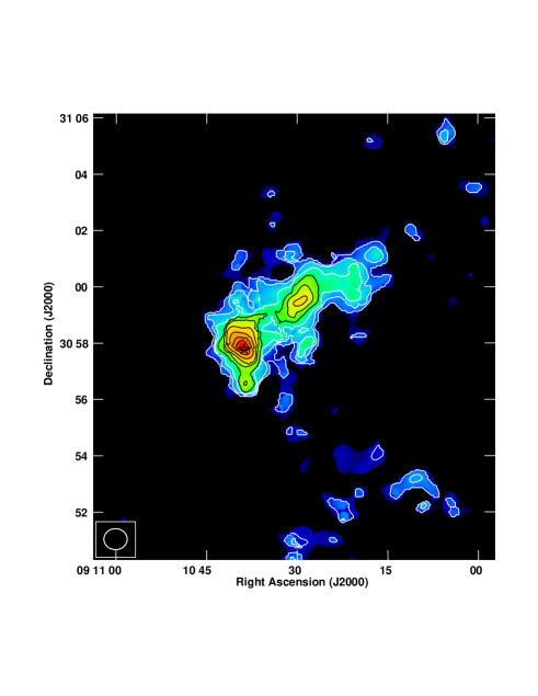
Figure 13: H i total intensity map, derived from data with 6 k$\lambda$ tapering (see Sect. 4.2). Contour levels are (1,2,3…9)$\times$6.6 Jy beam^-1 m s^-1. This image was derived by summing the emission over the velocity range from 2.6 to 11.6 km s^-1; to minimize the noise contribution to the map, data that did not exceed a 2$\sigma$ threshold after smoothing the data spatially and spectrally by a factor of 3 were blanked. The star symbol marks the stellar position of RS Cnc.

As previously reported by Matthews & Reid (2007), the H i associated with RS Cnc comprises two components: a compact structure centered close to the stellar position (the “head”), of size 75${}^{\prime\prime}\times$40^′′, and an extended wake of material that is known to trail directly opposite the direction of space motion of the star (the “tail”). The tail has a measured extent of $\sim 6^{\prime}$ ($\sim$0.25 pc) in the plane of the sky.

Based on Fig. 13 we find the peak H i column density within the “head” of RS Cnc, $\sim 16^{\prime\prime}$ north of RS Cnc (i.e., offset from the stellar position by roughly half a synthesized beam).

Our new H i data clearly confirm the previous suggestions that the H i emission surrounding the position of RS Cnc is elongated and that the position angle of this elongation is consistent with the CO outflow described above (see Matthews & Reid 2007; Libert et al. 2010). This is evident in the H i total intensity map (Fig. 13) and in the channel image centered at $V_{\rm LSR}=6.4$ km s^-1 (Fig. 12). Fig. 13 also shows evidence for two lobes of emission, extending north and south respectively from the more compact “head” of the H i emission structure. Each of these lobes extends to $\sim 100^{\prime\prime}$ from the stellar position. The correspondence between the elongation of the H i emission in RS Cnc’s head and the position angle of the molecular outflow traced in CO immediately suggest the possibility that the H i is tracing an extension of the molecular outflow beyond the molecular dissociation radius. An examination of the gas kinematics seems to reaffirm this picture (see Sect. 5.3).

Figure 14: Spatially integrated H i spectrum of RS Cnc derived from naturally-weighted (J)VLA C+D configuration data. The vertical bar indicates the stellar systemic velocity derived from CO observations. The spectral feature centered near the stellar systemic velocity is circumstellar in origin, while the second peak near $V_{\rm LSR}=-7$ km s^-1 results from interstellar contamination within the measurement aperture.

5.2 The Global H i Spectrum and Total H i Mass

An integrated H i spectrum of RS Cnc is shown in Fig. 14. The narrow, roughly Gaussian shape of the line profile is typical of many of the other AGB stars detected in H i (e.g., Gérard & Le Bertre 2006; Matthews et al. 2013), but it contrasts with the two-component CO line profile of RS Cnc (Fig. 3). The H i line centroid is also slightly offset from the stellar systemic velocity derived from the CO spectra (see Table 1), and as already seen from Fig. 12, the velocity range of the detected H i emission is significantly smaller than that of the CO emission. This suggests either that the atomic hydrogen has been slowed down by its interaction with the surrounding medium and/or that the material we detect in H i emission originated during an earlier epoch of mass loss during which the maximum outflow speeds were lower.

We have derived the velocity-integrated H i flux density for RS Cnc by integrating the emission in each spectral channel between 2.6-11.6 km s^-1 within a $6^{\prime}\,.8$$\times$$6^{\prime}\,.4$ rectangular aperture centered at the middle of the tail ($\alpha_{\rm J2000}=9^{\rm h}$ 10^m 29.8^s, $\delta_{\rm J2000}=30^{\circ}58^{\prime}$ $47^{\prime\prime}\,.3$). We use the naturally weighted data cube for this measurement, after correcting for the attenuation of the primary beam. Using this approach, we measure an integrated H i flux density $\int S_{\rm HI}dV=1.14\pm$0.03 Jy km s^-1. At our adopted distance to RS Cnc, this translates to an H i mass of 5.5$\times 10^{-3}\leavevmode\nobreak\ M_{\odot}$, where we have used the standard relation $M_{\rm HI}=2.36\times 10^{-7}d^{2}\int S_{\rm HI}dV$. Here $d$ is the distance in parsecs, $V$ is the velocity in km s^-1, and the units of $M_{\rm HI}$ are solar masses.

The integrated H i flux density that we derive for RS Cnc is a factor of $\sim$2.5 times higher than reported previously by Matthews & Reid (2007). We attribute this difference to a combination of three factors. First, the improved sensitivity and short spacing $u$-$v$ coverage of our combined C+D configuration data improves our ability to recover weak, extended emission. Secondly, Matthews & Reid measured the integrated emission within a series of irregularly shaped “blotches” in each spectral channel, defined by their outer 2$\sigma$ contours. While this approach minimizes the noise contribution to each measurement, it can also exclude weak, extended emission or noncontiguous emission features from the sum. Lastly, Matthews & Reid measured their integrated flux density from a tapered image cube. Based on the original VLA data alone, we found that for our presently adopted measurement aperture, this results in an integrated flux density that is $\sim$ 40% lower compared with a measurement from a naturally weighted data cube. Although our new H i mass estimate is higher than the previous value reported from VLA measurements, it is significantly less than reported by Libert et al. (2010) from NRT measurements ($M_{\rm HI}\approx 0.04\leavevmode\nobreak\ M_{\odot}$). We now suspect that the NRT measurement suffered from local confusion around 7 km s^-1.

Figure 15: H i position-velocity plot derived from naturally weighted data along PA=10^∘ and centered on the position of RS Cnc. Contour levels are ($-5.6$[absent],$-$4,$-$2.8,$-$2,2…5.6)$\times$1.1 mJy beam^-1. The lowest contour level is $\sim 2\sigma$. The origin of the $y$-axis is the stellar position.

5.3 Kinematics of the H i Emission

One of the key advantages of H i 21-cm line observations for the study of circumstellar ejecta is that they provide valuable kinematic information on material at large distances from the star. For example, for the AGB stars Mira and X Her, both of which have trailing H i wakes analogous to RS Cnc, Matthews et al. (2008) and Matthews et al. (2011), respectively, measured systematic velocity gradients along the length of the circumstellar wakes and used this information to constrain the timescale of the stellar mass-loss history (see also Raga & Cantó 2008). Interestingly, RS Cnc shows no clear evidence for a velocity gradient along the length of its wake. This can be seen simply from inspection of the channel maps in Fig.  12. RS Cnc also contrasts with the other stars known to have trailing H i wakes in that its space velocity is much lower, $\sim$15 km s^-1 compared with $V_{\rm space}\leavevmode\nobreak\ \hbox to0.0pt{$>$\hss}{\lower 4.30554pt\hbox{$\sim$}}$57 km s^-1 (see Matthews et al. 2013).

While no velocity gradient is seen along the tail of RS Cnc, the morphology of the tail gas reveals evidence for the importance of hydrodynamical effects. For example, a “wavy” structure is evident along the length of the tail in the channel image centered at $V_{\rm LSR}=6.4$ km s^-1 (Fig. 12). Additionally, the H i total intensity image in Fig. 13 shows a region of enhanced column density approximately half way long the length of this tail. A narrow stream of gas appears to connect this “presque isle” to the head of RS Cnc.

To facilitate comparison between the kinematics of the H i and CO emission in the CSE of RS Cnc, we present in Fig. 15 an H i position-velocity plot extracted along PA=10^∘—i.e., the position angle of the CO outflow described above. This plot shows that the kinematics of the atomic gas in the “head” of RS Cnc are rather complex.

We see that the central region of the head ($r\leavevmode\nobreak\ \hbox to0.0pt{$<$\hss}{\lower 4.30554pt\hbox{$\sim$}}\pm 50^{\prime\prime}$) contains emission spanning from $\sim$2 to 12 km s^-1—i.e., the full velocity range over which H i has been detected. However, all of the gas blueward of $\sim$4 km s^-1 lies north of the stellar position. This is suggestive of a relation to the high-velocity CO outflow, in which blueshifted emission is seen north of the star. Further, the velocity spread of the emission is smaller than seen in the molecular gas.

At distances of $>\pm 50^{\prime\prime}$ from RS Cnc, the gas kinematics appear different on the northern and southern sides of the head. In the south, we see evidence of H i emission near $V_{\rm LSR}\approx 6$ km s^-1 and $V_{\rm LSR}\approx 10$ km s^-1 extending to $\sim 100^{\prime\prime}$ from the stellar position. These features may represent the atomic counterparts to the south polar and equatorial molecular outflows, respectively. In the north, the high-latitude emission is dominated by a plume of gas whose velocity decreases from $\sim$9 km s^-1 at $\sim 50^{\prime\prime}$ north to $\sim$6 km s^-1 (close to the stellar systemic velocity) at $\sim 125^{\prime\prime}$ north. In Fig. 13 we see that the morphology and position angle of the emission at this location are suggestive of this being the extended northern counterpart to high-speed polar CO outflow. Alternatively, it could be material stripped from the equatorial regions.

6 Discussion

6.1 CO model

In Sect. 3.2, we have presented our preferred CO model, with a continuous density distribution from the equatorial plane to the poles. However, we tried several other configurations before selecting this model. Our first trial consisted in using directly the model proposed by Libert et al. (2010) of a bipolar flow and of an equatorial disk, separated by a gap, and with no velocity gradient in the outflows. The calculated spectra showed spikes at V_⋆ $\pm$ 2 km s^-1, and V_⋆ $\pm$ 6 km s^-1, corresponding to the velocities selected in the model (projected to the line of sight) whereas the observations reveal much smoother spectra. Also, the drifts in the velocities seen in the spectral maps were not reproduced.

In a second series, we introduced a gradient in the velocities in order to reproduce these drifts, all other parameters being kept identical. The agreement was generally improved, except for the central spectra. We have thus been led to subdivide the equatorial disk, introducing an inner part ($\pm$ 15^∘ of the equatorial plane) where the velocity is kept slow, and an outer part (from 30 to 45^∘, and from –30 to –45^∘) where the velocity is increased. Finally, as the gap between the equatorial disk and the polar outflows does not seem physically justified, we introduced smooth functions of the latitude for describing the velocity and the density, and obtained the results presented in Sect. 3.2. With this final step, the improvement on the sum of the square of the residuals was at least of a factor 2.

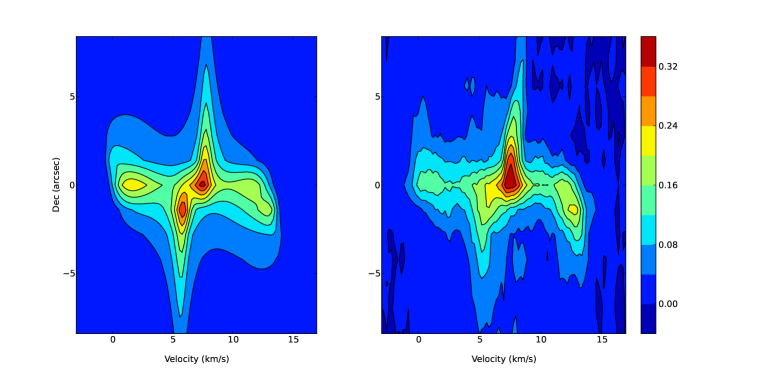
Figure 16: Left panel: synthetic position-velocity diagramme (offset in declination, from the 2000.0 Hipparcos position, against velocity) in CO1-0, obtained for our preferred model. The scale is in Jy/beam, and the channel width is 0.2 km s^-1. Right panel: observed position-velocity diagramme with same conditions.

One of the conclusions of these exercises is that the notion of a disk as a separate entity is perhaps misleading. The data are consistent with a low velocity outflow that extends in latitude far from the equatorial plane. On the other hand, a high velocity outflow along the polar direction is clearly needed. Although we cannot assert that our model is a unique representation of the close environment of RS Cnc, it is the simplest that we could find and that gives an approximate reproduction of the spectral maps available in CO1-0 and 2-1. The position-velocity diagrammes with two S-shaped features in opposition are often taken as evidence of disk/outflow structures (Nakashima 2005, Libert el al. 2010). In Fig. 16, we present the position (Dec)-velocity diagramme in CO1-0 obtained with our preferred model. The two S-shaped features are reproduced with the correct sizes and velocity amplitudes. It illustrates that our model can account as well for such a kind of diagramme.

The estimate of the mass loss rate that we obtain through our modeling agrees with that of Knapp et al. (1998, cf. Table 1), but not with that of Libert et al. (2010, 7.3 10^-7 M_⊙ yr^-1 at 143 pc). The latter assumed an optically thick wind in CO1-0, which, from the present work, appears unlikely. As discussed in Winters et al. (2003), this hypothesis may lead to an overestimate of the mass loss rate by a factor $\sim$ 3.5. We investigated the effect of the optical depth in our model, and found that self-absorption becomes effective only in the central part of the circumstellar shell in CO2-1. Furthermore, the CO2-1 and 3-2 spatially integrated spectra obtained by Knapp et al. are fitted satisfactorily by our model.

The simultaneous fit to the CO1-0, 2-1 and 3-2 data supports the temperature profiles adopted from Schöier & Olofsson (2010). However, we note that a steeper temperature profile would improve the quality of line-profile fits in the 2-1 spectral map, with almost no effect in 1-0. This is probably related to the fact that the 2-1 line starts to be optically thick for the lines of sight close to the central star. Clumpiness in the outflow could as well affect more the 2-1 data than the 1-0 ones.

An intriguing feature of the modeling is the need of a velocity gradient inside the CO shell. It is needed in order to reproduce the shifts in velocity of the blue and red peaks with distance to the central star. In a stationary case, it means that the outflow is still accelerated at distances larger than a few hundred AU (few 10¹⁵ cm). This is surprising because in models of dust-driven winds a terminal velocity is reached at a distance of $\sim$ 20 stellar radii (few 10¹⁴ cm, e.g. Winters et al. 2000). Other acceleration processes should probably be considered, for instance the radiation force on molecules (Jørgensen & Johnson 1992), which may play a role in low mass loss rate winds.

On the other hand, evidence of accelerating outflows has been obtained in some bipolar Pre-Planetary Nebulae. Recently Sahai et al. (2013) find a velocity gradient of 4 km s^-1 from $\sim$ 4$\times$10¹⁶ to 10¹⁷ cm in the ’waist’ of the low-luminosity (300 L_⊙) central star of the Boomerang Nebula (IRAS 12419–5414). Finally, although ad hoc, we cannot exclude that the flow is not stationary, and that we are witnessing a decrease with time of the expansion velocity.

In other CO-models, such as that of Schöier & Olofsson (2001), the expansion velocity is assumed to be constant throughout the CO shell. It is noteworthy that in these models the goal is to reproduce the spatially integrated spectra, and that turbulence is invoked with a typical value of $\sim$ 0.5 km s^-1 throughout the entire flow. In our modeling, we do not need to invoke turbulence.

6.2 binarity

The presence of Tc lines in its optical spectrum shows that RS Cnc is evolving on the TP-AGB, and that it has already undergone several thermal pulses and dredge-up events. Busso & Trippella (2013, personal communication), using recent prescriptions for mass loss (Cristallo et al. 2011) and the revision of the s-process element production by Maiorca et al. (2012), fitted the abundances and ¹²C/¹³C ratio determined by Smith & Lambert (1986) with a stellar evolution model of a 1.6 M_⊙ star in its 4th dredge-up episode. RS Cnc is clearly an intrinsic S-type star that does not owe its peculiar abundances to a mass transfer from a more evolved companion (Van Eck & Jorissen 1999).

The energy distribution of RS Cnc is presented in Fig. 17. It combines UV data from GALEX (at $\sim$ 154 and 232 nm), optical data from Mermilliod (1986), near-infrared data from 2MASS, far-infrared data from IRAS, and mm data from our work. There is no clear evidence of an UV excess that might reveal the presence of a warm companion. Also, we have found no evidence of a companion in the continuum map (Sect. 2.3). The CO structure at 6.6 km s^-1 (see Fig. 2) may hint to the presence of a companion that might be surrounded by a disk accreting material from the wind that would be seen only in a narrow range of velocities. In that case we would have a less evolved star, probably still on the main sequence, for instance a dwarf of less than 1.6 M_⊙. However, presently, we cannot discriminate between a clump in the outflow and a cloud around a companion.

In the course of the modeling process described in Sect. 6.1, we also introduced a disk in Keplerian rotation around the central star. There was no improvement of the quality of the fits and we did not include the rotating disk in our preferred model. It means that, presently, there is no evidence in the data of such a structure. However, we cannot exclude that new data with a better spatial resolution ($\leq$ 1^′′) would bring it into evidence. Such a structure has been invoked for X Her, another semi-regular AGB star with composite CO line-profiles, by Nakashima (2005), although it could not be confirmed by Castro-Carrizo et al. (2010).

Figure 17: Energy distribution of RS Cnc. The continuous line corresponds to a blackbody with size and temperature determined by Dumm & Schild (1998, see also Table 1).

The absence of evidence for a companion or a disk is puzzling. Another possibility for explaining the axi-symmetry in the outflow might be the rotation of the central star. Evidence for rotating cores in giant stars has recently been obtained by the satellites CoRoT and Kepler (e.g. Beck et al. 2012). These rotating cores might have an influence on the late mass loss of evolved stars when most of the stellar envelope has been removed. However, hydrodynamical models of stellar winds from rotating AGB stars predict a higher mass loss rate in the equatorial plane than in the polar directions (Dorfi & Höfner 1996, Reimers et al. 2000), which does not agree with our finding for RS Cnc (see Fig. 8). Finally, magnetic fields have been invoked for producing equatorial disks in AGB stars (e.g. Matt et al. 2010). These models result also in higher densities in the equatorial plane than in the polar directions, something that we do not observe.

6.3 ’head’ and ’tail’ in H i 

The ’head-tail’ structure revealed by the first observations of Matthews & Reid (2007) is reaffirmed. The global shape agrees with the triangular-shaped image obtained by Spitzer at 70 $\mu$m (Geise 2011), although the length of the IR tail ($\sim 4^{\prime}$) appears smaller than that in H i. This might be an effect of the temperature of the dust which is decreasing with distance to the central star, whereas the H i emission should not depend on temperature, and is thus a better tracer of morphology. Matthews et al. (2013) have classified the structures observed in H i around evolved stars in three categories. RS Cnc clearly belongs to Category 1 of “extended wakes, trailing the motions of the stars through space”, and resulting from the dynamical interaction between stellar winds and their local ISM.

Our new JVLA data show additional detail that makes RS Cnc the best observed case. The ’head’ is elongated in a direction consistent with the polar direction determined by the CO modeling. It corresponds to the direction in which the mass loss rate is maximum. However the velocity in H i is clearly smaller than in CO, which means that the outflow has been slowed down. Nevertheless, there is presently no observational evidence for a termination shock that would mark the external limit of the freely expanding wind (Libert et al. 2007). If it really exists it must be located between 20^′′ (or 4 10¹⁶ cm, the external limit of the CO wind), and 30^′′ (our spatial resolution at 21 cm).

The new data show also sub-structures in the ’tail’ that seem to be distributed in two groups, at $\sim 2.5^{\prime}$ and 5^′ from the star, that share the same elongated global shape as that of the ’head’. They could trace past episodes of enhanced mass loss. However the hydrodynamical models of the interaction between stellar outflows from evolved stars and the ISM tend to show that the wind variations do not remain recorded in the density or velocity structure of the gas (e.g. Villaver et al. 2002, 2012). Also the sub-structures observed in the ’tail’ are evocative of the vortices suggested by numerical simulations (Wareing et al. 2007). The presence of a latitude dependence of the stellar outflow may help to develop such sub-structures (Raga et al. 2008).

A particularity of RS Cnc ’tail’, as compared to the other objects in Category 1, is that there is no observed velocity gradient. It means that the tail of RS Cnc lies in the plane of the sky. This could be an effect of the small value of the stellar radial velocity. It also suggests that the local ISM shares the same radial velocity as RS Cnc. This hypothesis is supported by the ISM confusion which peaks at $\sim$ 7 km s^-1 (cf. figures 11 to 13 in Libert et al. 2010, and Sect. 5.2). If this is correct it would mean that the velocity of RS Cnc relative to its surrounding medium is still smaller than its space velocity (15 km s^-1).

The mass in atomic hydrogen is now estimated at 0.0055 M_⊙. Assuming 10% of the matter in He, it translates to 0.008 M_⊙. This does not account for a possible component of the ’head-tail’ in molecular hydrogen and/or ionized hydrogen. Given the effective temperature of RS Cnc (T_eff= 3226 K, Table 1), the presence of the former is unlikely (Glassgold & Huggins 1983).

Adopting the present mass loss rate estimated from the CO modeling, 1.24$\times$10^-7 M_⊙ yr^-1, we obtain a timescale of 64$\times$10³ years for the formation of the ’head-tail’ structure. This estimate should be used with caution, as we observe structures in the tail that might be due to episodes of enhanced mass loss. Also, models of stellar evolution generally predict a mass loss rate increasing with time.

The proper motions, corrected for solar motion (8 mas/yr in RA and 17 mas/yr in Dec), would translate to a crossing time of $\sim 2\times 10^{4}$ years for a 6^′ structure, a factor 3 less than the previous estimate. Therefore, the matter in the tail appears to follow the star in its motion through space, an effect that has already been observed in the other stars of Category 1 (e.g. Mira, Matthews et al. 2008).

Finally, the narrow linewidth ($\sim$ 4 km s^-1, Fig. 14) that is observed in H i can be used to constrain the temperature of the gas in the tail of RS Cnc. Assuming a Maxwellian distribution of the velocities and an optically thin emission, an H i line shows a Gaussian profile with a FWHM = 0.214$\times$T^1/2. We can thus estimate the average temperature in the tail at   $<$$\sim$ 350 K. As discussed above there is no global kinematics broadening of the H i line, because the tail lies in the plane of the sky, but there might be a contribution from vortices.

6.4 the multi-scale environment of RS Cnc

It is now possible to describe the RS Cnc outflow from $\sim$ 100 AU to its interface with the ISM at distances of tens of thousands of AU from the star. In the central part, the outflow exhibits an axi-symmetric morphology centered on the red giant. This structure develops on a scale $\geq$ 2000 AU, as probed by the CO lines. Our modeling shows that the flow is faster and more massive along the polar directions than in the equatorial plane. However, our present spatial resolution does not allow us to uncover the physical mechanism that shape the outflow close to the mass losing star, nor to evaluate the nature and the role of the sub-structure observed at 1^′′ northwest around 6.6 km s^-1.

The H i line at 21 cm enables us to trace the outflow beyond the molecular photodissociation radius. The flow is observed to be slowed down, and to keep the same preferential orientation, as observed in CO, over a distance of $\sim$ 8000 AU ($\sim$ 0.04 pc). Further away (from 0.04 pc to 0.25 pc) the flow is distorted by the motion relative to the local ISM. It takes the shape of a tail which is narrowing down stream, and shows sub-structures ($\sim$ 0.01 pc) that can be interpreted as vortices resulting from instabilities initiated at the level of a bow shock (Wareing et al. 2007). However the present spatial resolution is insufficient to observe the transition between the free-flowing stellar wind and the slowed-down flow in interaction with the ISM. Also, we do not observe directly the bow shock, perhaps because hydrogen from the ISM is ionized when crossing this interface (Libert et al. 2008).

Recent hydrodynamic models predict that tails similar to that observed around RS Cnc may develop in the early phase of mass loss from AGB stars (Villaver et al. 2003, 2012). However, they seem to be found preferentially in stars moving rapidly through the ISM ($\geq$ 50 km s^-1). The axi-symmetry of the central flow might also play a role in the development of red giant tails, as other stars which have a composite line-profile in CO show also an H i-tail (Matthews et al. 2008, 2011). The proximity of RS Cnc, the favorable observing conditions, and the well documented parameters of the system should allow us to perform a detailed comparison between observations and models.

7 Conclusions

New PdBI CO1-0 and JVLA H i interferometric data with higher spatial resolution have been obtained on the mass-losing semi-regular variable RS Cnc. These data combined with previous ones allow us to study with unprecedented detail the flow of gas from the central star to a distance of $\sim 10^{18}$ cm.

The previous CO observations of RS Cnc have been interpreted with a model consisting of an equatorial disk and a bipolar outflow. However, we find now that a better fit to the data can be obtained by invoking continuous axi-symmetric distributions of the density and the velocity, in which matter is flowing faster along the polar axis than in the equatorial plane. The polar axis is oriented at a position angle (PA) of 10^∘, and an inclination angle (from the plane of the sky) of 52^∘. It is aligned on the central AGB star. The mass loss rate is $\sim 1.24\times 10^{-7}$ M_⊙ yr^-1, with a flux of matter larger in the polar directions than in the equatorial plane. The axi-symmetry appears mainly in the velocity field and not in the density distribution. This probably implies that both stellar rotation and magnetic field are not the cause of the axi-symmetry. We also find that an acceleration of the outflow is possibly still at play at distances as large as 2$\times 10^{16}$ cm from the central star.

The H i data obtained at 21 cm with the (J)VLA show a ’head-tail’ morphology. The ’head’ is elongated in a direction consistent with the polar axis observed in the CO lines. The emission peaks close to the star with, at the present stage, no direct evidence of a termination shock. The 6^′-long tail is oriented at a PA of 305^∘, consistent with the proper motion of the star. It is resolved in several clumps that might develop from hydrodynamic effects linked to the interaction with the local interstellar medium. We derive a mass of atomic hydrogen of $\sim$ 0.0055 M_⊙, and the timescale for the formation of the tail $\sim$ 64$\times$ 10³ years, or more.

- (1) Adelman, S. J., & Dennis, J. W., 2005, Baltic Astronomy, 14, 41
- (2) Beck, P. G., Montalban, J., Kallinger, T., et al., 2012, Nature, 481, 55
- (3) Castro-Carrizo, A., Quintana-Lacaci, G., Neri, R., et al., 2010, A&A, 523, A59
- (4) Condon, J. J., Cotton, W. D., Greisen, E. W., et al., 1998, AJ, 115, 1693
- (5) Cotton, W. D., 2008, PASP, 120, 439
- (6) Cristallo, S., Piersanti, L., Straniero, O., et al., 2011, ApJS, 197, 17
- (7) Dorfi, E. A., & Höfner, S., 1996, A&A, 313, 605
- (8) Dumm, T., & Schild, H., 1998, New Astronomy, 3, 137
- (9) Famaey, B., Jorissen, A., Luri, X., et al., 2005, A&A, 430, 165
- (10) Gardan, E., Gérard, E., & Le Bertre, T., 2006, MNRAS, 365, 245
- (11) Geise, K. M., 2011, Master’s thesis, University of Denver
- (12) Gérard, E., & Le Bertre, T., 2006, AJ, 132, 2566
- (13) Glassgold, A. E., & Huggins, P. J., 1983, MNRAS, 203, 517
- (14) Greisen, E. W., 2003, Information Handling in Astronomy—Historical Vistas, ed. A. Heck (Dordrecht: Kluwer), 109
- (15) James, F., & Roos, M., 1975, Comput. Phys. Commun., 10, 343
- (16) Jørgensen, U. G., & Johnson, H. R., 1992, A&A, 265, 168
- (17) Knapp, G. R., Young, K., Lee, E., & Jorissen, A., 1998, ApJS, 117, 209
- (18) Lebzelter, T., & Hron, J., 1999, A&A, 351, 533
- (19) Libert, Y., Gérard, E., & Le Bertre, T., 2007, MNRAS, 380, 1161
- (20) Libert, Y., Le Bertre, T., Gérard, E., & Winters, J. M., 2008, Proc. SF2A-2008, C. Charbonnel, F. Combes & R. Samadi (eds.), p. 317
- (21) Libert, Y., Winters, J. M., Le Bertre, T., Gérard, E., & Matthews, L. D., 2010, A&A, 515, A112
- (22) Maiorca, E., Magrini, L., Busso, M., Randich, S., Palmerini, S., & Trippella, O., 2012, ApJ, 747, 53
- (23) Mamon, G. A., Glassgold, A. E., & Huggins, P. J., 1988, ApJ, 328, 797
- (24) Matthews, L. D., Le Bertre, T., Gérard, E., & Johnson, M. C., 2013, AJ, 145, 97
- (25) Matt, S., Balick, B., Winglee, R., & Goodson, A., 2010, ApJ, 545, 965
- (26) Matthews, L. D., Le Bertre, T., Gérard, E., Johnson, M. C., & Dame, T. M., 2011, AJ, 141, 60
- (27) Matthews, L. D., Libert, Y., Gérard, E., Le Bertre, T., & Reid, M. J., 2008, ApJ, 684, 603
- (28) Matthews, L. D., & Reid, M. J., 2007, AJ, 133, 2291
- (29) Mermilliod, J.-C., 1986, Catalogue of Eggen’s UBV data
- (30) Nakashima, J., 2005, ApJ, 620, 943
- (31) Neri, R., Kahane, C., Lucas, R., Bujarrabal, V., & Loup, C., 1998, A&AS, 130, 1
- (32) Nguyen-Q-Rieu, Laury-Micoulaut, C., Winnberg, A., & Schultz, G. V., 1979, A&A, 75, 351
- (33) Perley, R. A., 2010, EVLA Memo 145, http://www.aoc.nrao.edu/evla/geninfo/ memoseries/evlamemo145.pdf
- (34) Perley, R. A., Chandler, C. J., Butler, B. J., & Wrobel, J. M., 2011, ApJ, 739, L1
- (35) Perryman, M. A. C., Lindegren, L., Kovalevsky, J., et al., 1997, A&A, 323, L49
- (36) Raga, A. C., & Cantó, J., 2008, ApJ, 685, L141
- (37) Raga, A. C., Cantó, J., De Colle, F., Esquivel, A., Kajdic, P., Rodríguez-González, A., & Velázquez, P. F., 2008, ApJ, 680, L45
- (38) Ramstedt, S., Schöier, F. L., Olofsson, H., & Lundgren, A. A., 2008, A&A, 487, 645
- (39) Reimers, C., Dorfi, E. A., & Höfner, S., 2000, A&A, 354, 573
- (40) Sahai, R., Morris, M., Sánchez Contreras, C., & Claussen, M., 2007, AJ, 134, 2200
- (41) Sahai, R., Vlemmings, W. H. T., Huggins, P. J., Nyman, L.-Å., & Gonidakis, I., 2013, ApJ, 777, 92
- (42) Schöier, F. L., & Olofsson, H., 2001, A&A, 368, 969
- (43) Schönrich, R., Binney, J., & Dehnen, W., 2010, MNRAS, 403, 1829
- (44) Smith, V. V., & Lambert, D. L., 1986, ApJ, 311, 843
- (45) Stephenson, C. B., 1984, Publ. Warner & Swasey Obs., 3, 1
- (46) Van Eck, S., & Jorissen, A., 1999, A&A, 345, 127
- (47) van Leeuwen, F., 2007, ”Hipparcos, the New Reduction of the Raw Data”, Springer, Astrophysics and Space Science Library, vol. 350
- (48) Villaver, E., García-Segura, G., & Manchado, A., 2002, ApJ, 571, 880
- (49) Villaver, E., García-Segura, G., & Manchado, A., 2003, ApJ, 585, L49
- (50) Villaver, E., Manchado, A., & García-Segura, G., 2012, ApJ, 748, 94
- (51) Wareing, C. J., Zijlstra, A. A., & O’Brien, T. J., 2007, ApJ, 660, L129
- (52) Winters, J. M., Le Bertre, T., Jeong, K. S., Helling, C., & Sedlmayr, E., 2000, A&A, 361, 641
- (53) Winters, J. M., Le Bertre, T., Jeong, K. S., Nyman, L.-Å., & Epchtein, N., 2003, A&A, 409, 715