Quasi-geostrophic approximation of anelastic convection

Abstract

The onset of convection in a rotating cylindrical annulus with parallel ends filled with a compressible fluid is studied in the anelastic approximation. Thermal Rossby waves propagating in the azimuthal direction are found as solutions. The analogy to the case of Boussinesq convection in the presence of conical end surfaces of the annular region is emphasised. As in the latter case the results can be applied as an approximation for the description of the onset of anelastic convection in rotating spherical fluid shells. Reasonable agreement with three-dimensional numerical results published by Jones et al. (J. Fluid Mech., vol. 634, 2009, pp. 291-319) for the latter problem is found. As in those results the location of the onset of convection shifts outwards from the tangent cylinder with increasing number $N_{\rho}$ of density scale heights until it reaches the equatorial boundary. A new result is that at a much higher number $N_{\rho}$ the onset location returns to the interior of the fluid shell.

(a)	(b)

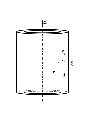
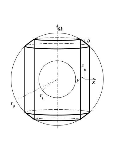
Figure 1: Sketch of geometric configurations. (a) The rotating cylindrical annulus with parallel ends considered in §2 as a model of the effect of background density variation. (b) The rotating cylindrical annulus with conical ends inscribed in a spherical shell. The sketches are not to scale with the asymptotic limit assumptions.

1 Introduction

The tendency of fluid motions in rapidly rotating systems to develop nearly two-dimensional structures has often been exploited to simplify the theoretical analysis. The description of convection flows in systems where the gravity vector and the rotation axis are not parallel provides a typical example (Busse, 1970, 2002). In applications of convection problems to rotating planets and stars the tendency towards two-dimensionality is partly obscured by the strong variation of fluid density as a function of radius in the nearly spherical systems. It is thus of interest to investigate the extent to which the quasi-geostrophic two-dimensional description can still provide an approximation for three-dimensional convection in rapidly rotating systems with strong variations of density.

In the case of the Boussinesq approximation, in which the density is regarded as constant except in connection with the gravity term, the results derived from the two-dimensional quasi-geostrophic analysis of the onset of convection in rotating spherical fluid shells compare well with the results of the three-dimensional numerical analysis (Simitev & Busse, 2003). In this paper the two-dimensional model was based on the problem of convection in a rotating cylindrical annulus with conical end boundaries (Busse, 1970, 1986). For a more detailed discussion of the role of the quasi-geostrophic model in relationship to more accurate three-dimensional solutions for convection in rotating spherical fluid shells we refer to the paper of Gillet & Jones (2006).

In recent years the anelastic approximation (Gough, 1969) has been widely used to obtain more realistic descriptions of convection in the atmospheres of planets and stars with strong variations of density. In the paper by Busse (1986, hereafter B86), the analogy between the effect of changing height induced by the conical boundaries of the cylindrical annulus and the effect of a radial variation of density has already been pointed out. In the present paper we intend to demonstrate quantitatively that the two-dimensional analysis of the annulus model provides a reasonable approximation for the onset of convection in the presence of strong anelastic density variations in rotating spherical fluid shells.

The analysis of the present paper resembles to some extent the two-dimensional analysis of anelastic convection pursued by Evonuk & Glatzmaier (2004, 2006); see also Glatzmaier et al. (2009). Because of the high computational cost of three-dimensional simulations of convection in the presence of density variation over many scale heights these authors restricted their attention to two-dimensional numerical simulation of convection close to the equatorial plane. Evonuk & Glatzmaier were interested in the nonlinear properties of two-dimensional convection including zonal flows in the presence of strong density variations. In contrast, our analytical model focuses on the linear problem of the onset of convection at high values of the rotation parameter.

The main purpose of this paper is not the demonstration of a high accuracy of the two-dimensional approximation. Instead we wish to emphasise the insights into anelastic convection in rotating spheres gained from the analytical quasi-geostrophic model. In the next section we first introduce the narrow-gap cylindrical annulus with parallel ends as shown in figure 1(a) and derive the two-dimensional solution describing anelastic convection. In §3 the model is modified for applications to the onset of anelastic convection in rotating spherical shells as indicated in figure 1(b). Detailed comparisons with numerical solutions are evaluated in §4. Some nonlinear aspects are discussed in the final §of the paper.

2 Mathematical description of two-dimensional anelastic convection

We consider a cylindrical annulus with parallel ends rotating about its axis with the angular velocity $\Omega$ as shown in figure 1(a). The gap width $d$ in the radial direction of the annular region is small in comparison with its inner radius $r_{i}$ such that a cartesian system of dimensionless coordinates $x,y,z$ in the radial, azimuthal and axial directions, respectively, can be used for a local description of convection. The corresponding unit vectors are $\mbox{\boldmath$i$},\mbox{\boldmath$j$}$ and $k$. The annular gap is filled with an ideal gas the state of which differs little from an isentropic reference state in the presence of gravity pointing in the negative $x$-direction. The small deviation from the isentropic state is described by the small positive excess entropy $\Delta s$ by which the entropy at the inner cylinder exceeds the entropy at the outer cylindrical boundary. In experimental realisations gravity could be replaced by the centrifugal force. The dynamical problem would then be identical if a negative value of $\Delta s$ is assumed.

Using $d$ as length scale, $d^{2}/\kappa$ as time scale and $\Delta s$ as the scale of the entropy we obtain the dimensionless form of the anelastic equations as used in (Jones et al., 2009) and in the benchmark paper (Jones et al., 2011) based on the formulation introduced independently by Lantz & Fan (1999) and Braginsky & Roberts (1995),

$$\frac{\partial\mbox{\boldmath$u$}}{\partial t}+\mbox{\boldmath$u$}\cdot\boldsymbol{\nabla}\mbox{\boldmath$u$}+\tau\mbox{\boldmath$k$}\times\mbox{\boldmath$u$}=-\boldsymbol{\nabla}\pi+\mbox{\boldmath$i$}\frac{{\mathit{R}}}{{\mathit{Pr}}}s+\mbox{\boldmath$F$},$$ (2.1a)

$$\boldsymbol{\nabla}\cdot\mbox{\boldmath$u$}=\bar{\rho}\mbox{\boldmath$u$}\cdot\boldsymbol{\nabla}\frac{1}{\bar{\rho}},$$ (2.1b)

$${\mathit{Pr}}\left(\frac{\partial s}{\partial t}+\mbox{\boldmath$u$}\cdot\boldsymbol{\nabla}s\right)=\boldsymbol{\nabla}^{2}s+\boldsymbol{\nabla}s\cdot\frac{1}{\kappa\bar{\rho}\overline{T}}\boldsymbol{\nabla}\kappa\bar{\rho}\overline{T}+\hat{Q},$$ (2.1c)

where $F$ denotes the force of viscous friction divided by the density, and all terms in the equation of motion that can be written as gradients have been combined into $\boldsymbol{\nabla}\pi$. The Rayleigh number ${\mathit{R}}$, the Prandtl number ${\mathit{Pr}}$ and the Coriolis number $\tau$ are defined by

$${\mathit{R}}=\frac{gd^{3}\Delta s}{\kappa\nu c_{p}},\hskip 28.45274pt{\mathit{Pr}}=\frac{\nu}{\kappa},\hskip 28.45274pt\tau=2\Omega\frac{d^{2}}{\nu}.$$ (2.2)

Here $\kappa$ is the entropy diffusivity, $\nu$ is the kinematic viscosity and $c_{p}$ is the specific heat at constant pressure. For simplicity we have assumed that material properties are constant except for $\bar{\rho}(x)$, which represents the $x$-dependent density of the isentropic reference state made dimensionless through division by its average value, and $\overline{T}(x)$ is the temperature profile of that state. The constant gravity vector is given by $\mbox{\boldmath$g$}=-g\mbox{\boldmath$i$}$, and the entropy $s$ can be separated into two parts,

$$s=-x+\tilde{s},$$ (2.3)

such that the boundary condition $\tilde{s}=0$ holds at $x=\pm 1/2$.

We now consider two-dimensional solutions of equations (2.1) that are independent of $z$ and thus satisfy the Proudman-Taylor condition. Assuming $\mbox{\boldmath$u$}=(1/\bar{\rho})\boldsymbol{\nabla}\psi(x,y,t)\times\mbox{\boldmath$k$}$ we obtain for the $z$ component of the vorticity of equation (2.1a)

$$\frac{\partial\zeta}{\partial t}+\frac{1}{\bar{\rho}}\left(\frac{\partial\zeta}{\partial x}\frac{\partial\psi}{\partial y}-\frac{\partial\zeta}{\partial y}\frac{\partial\psi}{\partial x}-(\tau+\zeta)\frac{1}{\bar{\rho}}\frac{d\bar{\rho}}{dx}\frac{\partial\psi}{\partial y}\right)=-\frac{{\mathit{R}}}{{\mathit{Pr}}}\frac{\partial\tilde{s}}{\partial y}+\Delta_{2}\zeta,$$ (2.4)

where $\zeta=\mbox{\boldmath$k$}\cdot\boldsymbol{\nabla}\times\big{(}(\boldsymbol{\nabla}\psi\times\mbox{\boldmath$k$})/\bar{\rho}\big{)}$ is the $z$ component of the vorticity and $\partial^{2}/\partial x^{2}+\partial^{2}/\partial y^{2}$ has been denoted by $\Delta_{2}$. Following Evonuk & Glatzmaier (2004) the friction term has been reduced to its main contributor. Assuming that $\bar{\rho}$ varies slowly such that the absolute value of

$$\eta_{\rho}\equiv-\frac{1}{\bar{\rho}}\frac{d\bar{\rho}}{dx}$$ (2.5)

is a small constant we find that the absolute value of

$$\eta_{\rho}^{*}\equiv\eta_{\rho}\tau$$ (2.6)

is a parameter of the order unity or larger for $\tau\gg 1$. In fact, later we shall consider the limit of $\eta_{\rho}^{*}$ tending to infinity.

We thus have arrived at the same equations as in the case of Boussinesq convection in the annulus with conical end boundaries (see figure 1(b)) given by (4.1) of B86 with the only difference that the second and third terms on the right-hand side of equation (2.1c) are missing in the latter case. In the following we shall neglect these two terms anticipating that they become negligible in the asymptotic solution of the problem for $\tau$ tending to infinity.

(a)	(b)

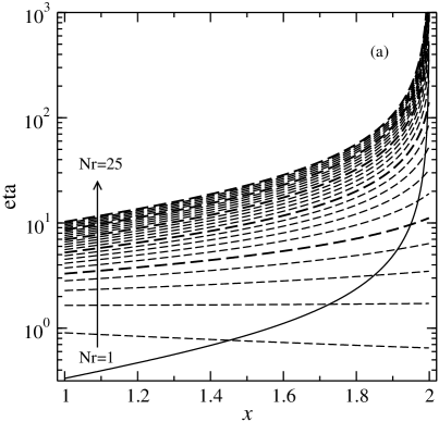
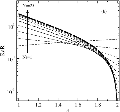
Figure 2: (a) The functions $\eta^{*}/\tau$ given by (3.1) (solid line) and $\eta_{\rho}^{*}/\tau$ given by (3) (dashed lines), and (b) the factor ${\mathit{Ra}}/{\mathit{R}}$ given by (3.4) in dependence of $x$ in the case $n=2$, $\beta=0.5$ and $N_{\rho}=1,2,\dotsc,25$ increasing in the direction of the arrows with the thicker dashed lines corresponding to $N_{\rho}=5,10,15,20,25$.

The linearised versions of equations (2.1c) and (2.4) thus assume the forms

$$\frac{\partial\zeta}{\partial t}+\frac{\eta_{\rho}^{*}}{\bar{\rho}}\frac{\partial\psi}{\partial y} =-\frac{{\mathit{R}}}{{\mathit{Pr}}}\frac{\partial\tilde{s}}{\partial y}+\Delta_{2}\zeta,$$ (2.7a)

$${\mathit{Pr}}\frac{\partial\tilde{s}}{\partial t}-\frac{{\mathit{Pr}}}{\bar{\rho}}\frac{\partial\psi}{\partial y} =\Delta_{2}\tilde{s}.$$ (2.7b)

After elimination of $\tilde{s}$, neglecting terms of the order of $\eta_{\rho}$, and multiplication of the equation of motion by $\bar{\rho}$ we obtain

$$\left({\mathit{Pr}}\frac{\partial}{\partial t}-\Delta_{2}\right)\left[\Big{(}\frac{\partial}{\partial t}-\Delta_{2}\Big{)}\Delta_{2}-\eta_{\rho}^{*}\frac{\partial}{\partial y}\right]\psi={\mathit{R}}\frac{\partial^{2}}{\partial y^{2}}\psi.$$ (2.8)

This equation is easily solved when stress-free conditions at the boundaries $x=\pm 1/2$ are assumed,

$$\psi=\sin\big{(}\pi(x+1/2)\big{)}\exp(i\alpha y-i\omega t),\hskip 28.45274pt\tilde{s}=\frac{-i\alpha\psi}{-i\omega{\mathit{Pr}}+\alpha^{2}+\pi^{2}}.$$ (2.9)

This solution yields the dispersion relation

$${\mathit{R}}\alpha^{2}=(-i\omega{\mathit{Pr}}+\alpha^{2}+\pi^{2})\big{[}(-i\omega+\alpha^{2}+\pi^{2})(\alpha^{2}+\pi^{2})+i\alpha\eta_{\rho}^{*}\big{]}.$$ (2.10)

The real and imaginary parts of this equation determine the neutral curve ${\mathit{R}}(\alpha)$ and the frequency ${\mathit{\omega}}(\alpha)$ of the thermal Rossby wave,

$${\mathit{\omega}}=\frac{\alpha\eta_{\rho}^{*}}{(1+{\mathit{Pr}})(\alpha^{2}+\pi^{2})},\hskip 14.22636pt{\mathit{R}}=(\alpha^{2}+\pi^{2})^{3}\alpha^{-2}+\left(\frac{\eta_{\rho}^{*}{\mathit{Pr}}}{1+{\mathit{Pr}}}\right)^{2}/(\alpha^{2}+\pi^{2}).$$ (2.11)

The angular frequency ${\mathit{\omega}}$ resembles that of ordinary Rossby waves from which it differs only through the appearance of ${\mathit{Pr}}$ in the denominator. The Rayleigh number is determined by two terms. The first is the familiar expression from Rayleigh-Bénard convection which is independent of the Coriolis number. The second term is introduced by the density variation caused by the compressibility.

The critical value $\mathit{R_{c}}$ and the corresponding wavenumber $\mathit{\alpha_{c}}$ are obtained through minimising ${\mathit{R}}(\alpha)$ with respect to $\alpha$ which yields in the limit of high values of $|\eta_{\rho}^{*}|$

$$\mathit{\alpha_{c}}={\mathit{\eta_{P}}}^{1/3}(1-\frac{7}{12}\pi^{2}{\mathit{\eta_{P}}}^{-2/3}+\dots),\hskip 28.45274pt\mathit{R_{c}}={\mathit{\eta_{P}}}^{4/3}(3+\pi^{2}{\mathit{\eta_{P}}}^{-2/3}+\dots),$$ (2.12)

where ${\mathit{\eta_{P}}}$ is defined by

$${\mathit{\eta_{P}}}\equiv\frac{|\eta_{\rho}^{*}|{\mathit{Pr}}}{\sqrt{2}(1+{\mathit{Pr}})}.$$ (2.13)

As in the Boussinesq case of the cylindrical annulus with conical axial boundaries, the onset of convection becomes independent of the gap width $d$ in the limit of high $|\eta_{\rho}^{*}|$ and the Rayleigh numbers for modes with $\sin\big{(}l\pi(x+1/2)\big{)}$ with $l=2,3,4,\dotsc$ hardly differ from that for $l=1$. The neglected second term on the right-hand side of equation (2.1c) would contribute only a negligible amount in the limit of high $\mathit{\alpha_{c}}$. The other neglected term $\hat{Q}$ does not enter the linear problem, of course.

The fact that the asymptotic relationship $\mathit{R_{c}}=3\mathit{\alpha_{c}}^{4}$ holds independently of the choice of length scale for a given entropy gradient is essential for the following analysis. In other words, the only remaining physical length scale in the limit

$$\eta_{P}^{1/3}\gg 1$$ (2.14)

is the dimensional azimuthal wave length $\lambda_{D}$ of convection which must be small compared to any radial length scale of the problem. In terms of dimensional quantities the condition (2.14) translates into the condition that the asymptotic expression for $\lambda_{D}$,

$$\lambda_{D}\equiv 2\pi\left(\frac{\kappa\sqrt{2}(1+{\mathit{Pr}})\overline{\rho}}{2\Omega\left(\displaystyle\frac{d}{dx_{D}}\overline{\rho}\right)}\right)^{1/3}$$ (2.15)

is small compared to any radial length scale of the problem, where $x_{D}$ denotes the dimensional length on which $\overline{\rho}$ varies.

(a)	(b)

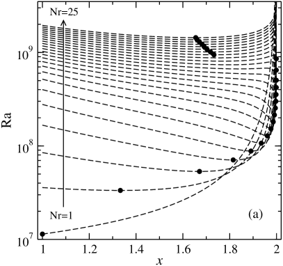
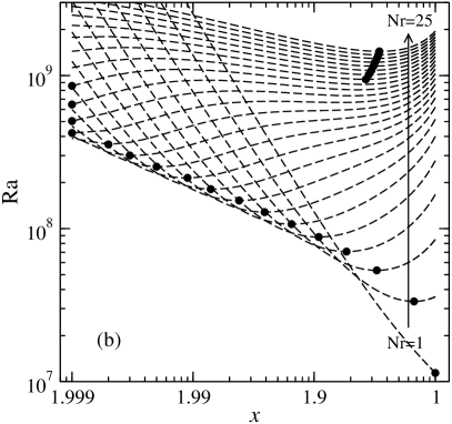
Figure 3: Critical Rayleigh number as a function of position $x$ in the cases $\beta=0.5$, ${\mathit{Pr}}=1$, $\tau=10^{5}$, $n=2$ and $N_{\rho}=1,2,\dotsc,25$ increasing in the direction of the arrows. The black dots indicate the position of the minimum on each curve. Panels (a) and (b) are identical only the $x$-axis is scaled differently to reveal the structure near the outer boundary.

3 Application to three-dimensional geometries

In applying the two-dimensional solution to a three-dimensional configuration we follow the corresponding analysis (Busse, 1970) in the case of Boussinesq convection. In particular, we shall consider the case of a rotating spherical fluid shell as shown in figure 1(b). Since we are using only the asymptotic results of §2 which are independent of the radial length scale $d$ in the formulation of the problem, we are free to interpret $d$ from now on as the thickness of the spherical shell. Accordingly the inner and outer radii, $r_{i}$ and $r_{o}$, are given by $\beta/(1-\beta)$ and $1/(1-\beta)$, respectively, where $\beta$ is defined by $\beta=r_{i}/r_{o}$.

Simitev & Busse (2003) have demonstrated that a good approximation for the onset of convection in rotating spherical shells can be obtained by solutions of the form (3.8)–(3.10) in B86 found from the model of the rotating annulus with conical ends. In the spherical case the parameter $\eta^{*}$ is defined by

$$\eta^{*}\equiv\frac{\tau\tan\theta}{r_{o}\cos\theta}=\frac{\tau x}{r_{o}^{2}-x^{2}}.$$ (3.1)

where $\theta$ is the colatitude on the spherical surface with respect to the axis of rotation and $x=r_{o}\sin\theta$ represents the distance from the axis at which convection sets in. Although the analysis leading to the results (2.11) and (2.12) with $\eta^{*}_{\rho}$ replaced by $\eta^{*}$ as shown in B86 is mathematically rigorous only in the limit of small $\theta$, the asymptotic expressions compare quite well with the numerical results at finite angles $\theta$. A further improvement may eventually be obtained following Calkins et al. (2013) who replaced the two-dimensional procedure by a three-dimensional one.

In the presence of density variation the contribution $\eta_{\rho}^{*}$ as defined in the preceding section must be added. Since the density in the spherical configuration varies not only with distance from the axis, but also parallel to the axis, an average over the latter dimension must be taken. The same procedure must be applied to gravity. In order to compare our analytical results with the direct numerical results of Jones et al. (2009), we shall use the following explicit expressions defined in (Jones et al., 2009, 2011):

$$\bar{\rho}\equiv\xi^{n}\quad\mbox{with}\quad\xi=c_{0}+c_{1}/r,$$ (3.2)

$$\mbox{and with}\quad c_{0}=\frac{2\xi_{o}-\beta-1}{1-\beta},\quad c_{1}=\frac{(1+\beta)(1-\xi_{o})}{(1-\beta)^{2}},$$

$$\mbox{where}\quad\xi_{i}=\frac{\beta+1-\xi_{o}}{\beta}\quad\mbox{and}\quad\xi_{o}=\frac{\beta+1}{\beta\exp(N_{\rho}/n)+1}$$

are the values of $\xi$ at the inner and outer boundaries. Here $N_{\rho}$ is the number of density scale heights, $N_{\rho}=n\ln(\xi_{i}/\xi_{o})$, and $n$ is the gas polytropic index.

(a)	(b)

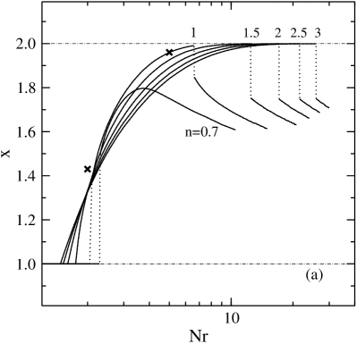
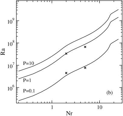
Figure 4: (a) The position of the minimal critical Rayleigh number, ${\mathit{Ra_{c}}}$, as a function of $N_{\rho}$ for the case $\beta=0.5$, ${\mathit{Pr}}=1$, $\tau=10^{5}$ with $n$ as indicated in the plot. (b) The minimal critical Rayleigh number, ${\mathit{Ra_{c}}}$, as a function of $N_{\rho}$ for $\beta=0.5$, $\tau=10^{5}$, $n=2$ and ${\mathit{Pr}}=0.1,1,10$ as indicated in the plot. The crosses show values obtained by Jones et al. (2009) from direct numerical solution of the linearised spherical problem with $n=2$.

The definitions (2.5) and (2.6) thus become modified to

$$\begin{aligned} \eta^{*}_{\rho}&=-\frac{\tau}{\sqrt{r_{o}^{2}-x^{2}}}\int\limits_{0}^{\sqrt{r_{o}^{2}-x^{2}}}\frac{d}{dx}\ln\Big{(}\bar{\rho}\big{(}\sqrt{x^{2}+z^{2}}\big{)}\Big{)}dz\\ &=\frac{n\tau}{\sqrt{r_{o}^{2}-x^{2}}}\int\limits_{0}^{\sqrt{r_{o}^{2}-x^{2}}}\frac{c_{1}xdz}{(c_{0}\sqrt{x^{2}+z^{2}}+c_{1})(x^{2}+z^{2})}.\end{aligned}$$

An analytical expression for this integral can be obtained, but it is lengthy and will not be given here. The parameters $\eta^{*}$ and $\eta^{*}_{\rho}$ are displayed as functions of $x$ in figure 2(a) in the special case $n=2$, $\beta=0.5$.

In order to apply the two-dimensional approximation to the three-dimensional formulation used by Jones et al. (2009, 2011), we must take into account that the entropy gradient of the purely conducting state is spatially dependent and that the same holds for the gravity term which in (Jones et al., 2009, 2011) is assumed to vary in proportion to $r^{-2}$. For the cylindrical approximation only the component perpendicular to the axis of rotation is relevant. For this component in the formulation of Jones et al. (2009, 2011), we get in place of ${\mathit{R}}$ in equation (2.8)

$${\mathit{Ra}}\frac{x}{r}\frac{\Delta s}{r^{2}}\left[\frac{nc_{1}x}{r^{3}\xi^{n+1}}\frac{1}{\xi_{o}^{-n}-\xi_{i}^{-n}}\right],$$ (3.3)

where the term inside the square brackets denotes the negative $x$ derivative of the entropy in the motionless purely conducting state. The average of expression (3.3) over the cylindrical surface intersecting the spherical shell at the distance $x$ from the axis thus leads to the ratio between the Rayleigh number ${\mathit{R}}$ of the cylindrical model and the Rayleigh number ${\mathit{Ra}}$ introduced by Jones et al. (2009, 2011) in the spherical case

$$\frac{{\mathit{R}}}{{\mathit{Ra}}}=\frac{nc_{1}x^{2}}{\sqrt{r_{o}^{2}-x^{2}}}\int_{0}^{\sqrt{r_{o}^{2}-x^{2}}}\frac{dz}{(x^{2}+z^{2})^{3}(c_{0}+c_{1}/\sqrt{x^{2}+z^{2}})^{n+1}(\xi_{o}^{-n}-\xi_{i}^{-n})}.$$ (3.4)

The reciprocal of this function which is independent of $\tau$ and ${\mathit{Pr}}$ has been plotted in figure 2(b) in the special case $n=2$, $\beta=0.5$.

4 Comparison of the asymptotic results with numerical data

In this section the asymptotic results derived above will be compared with numerical data found in the literature for the onset of anelastic convection in rapidly rotating spherical shells. The goal of this comparison is not to demonstrate an optimal quantitative agreement, but to show that the asymptotic expressions reflect all qualitative properties of the numerical results quite well and can thus be used for explorations of regions of parameter space that may not be easily accessible to direct numerical integrations.

(a)	(b)

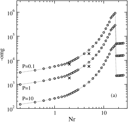
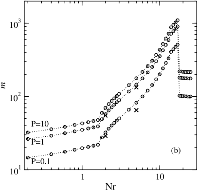
Figure 5: (a) The global critical frequency $\omega_{c}$ and (b) the critical azimuthal wave number $m_{\text{crit}}$ as a function of $N_{\rho}$ for $\beta=0.5$, $\tau=10^{5}$, $n=2$ and ${\mathit{Pr}}=0.1,1,10$ as indicated in the plot. The crosses show values obtained by Jones et al. (2009) from direct numerical solution of the linearised spherical problem.

Combining the effect of the density stratification (3) and that of the boundary inclination (3.1) at the spherical surface we find

$${\mathit{\eta_{P}}}(x)\equiv\frac{|\eta^{*}_{\rho}+\eta^{*}|{\mathit{Pr}}}{\sqrt{2}(1+{\mathit{Pr}})},$$ (4.1)

yielding the asymptotic critical values for the azimuthal wavenumber $\mathit{\alpha_{c}}$ and for the Rayleigh number $\mathit{R_{c}}(x)$

$$\mathit{\alpha_{c}}(x)=\eta^{1/3}_{P}(x),\hskip 56.9055pt\mathit{R_{c}}(x)=3\eta^{4/3}_{P}(x).$$ (4.2)

The dependence of $\mathit{R_{c}}(x)$ on the fourth power of $\mathit{\alpha_{c}}$ demonstrates again that it is independent of the chosen length scale $d$. The characteristic length of convection is given by its azimuthal wavelength which does not depend on any radial length scale in the asymptotic limit. This property is also evident from figure 2 of Jones et al. (2009) in which the radial extent of the convection columns does not reflect any connection with the thickness $d$ of the spherical fluid shell.

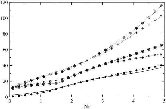
Figure 6: Comparison with direct numerical results shown in figure 1(a) of Jones et al. (2009). The values ${\mathit{Ra_{c}}}\times 10^{-5}$, $m_{\text{crit}}$ and $\omega_{\text{crit}}\times 10^{-1}$ reported by Jones et al. (2009) (solid line, stars and plus-signs, respectively) are plotted against the corresponding values of ${\mathit{Ra_{c}}}\times 10^{-5}$, $m_{\text{crit}}$ and $2/3\times\omega_{c}\times 10^{-1}$ obtained from our analysis (bold dots, circled stars and circled plus-signs, respectively). The factor 2/3 in front of the values of $\omega_{c}$ obtained from expression (4.4) has been introduced to facilitate the comparison of the shapes of the two frequency curves. The values of the parameters are ${\mathit{Pr}}=1$, $\tau=10^{4}$, $n=2$, $\beta=0.5$ and $N_{\rho}$ varies along the abscissa.

The value ${\mathit{Ra}}(x)$ is obtained through application of relationship (3.4). This function is plotted in figure 3 for various values of $N_{\rho}$ in the case $\beta=0.5,\tau=10^{5},n=2$ for the Prandtl number ${\mathit{Pr}}=1$. For ${\mathit{Pr}}=0.1$ the same plots are obtained except that the Rayleigh number is decreased by the factor $(0.2/1.1)^{4/3}$ as follows from the asymptotic dependence $\big{(}{\mathit{Pr}}/(1+{\mathit{Pr}})\big{)}^{4/3}$ of the Rayleigh number on the Prandtl number. While the values indicate some quantitative discrepancies with the data displayed in (Jones et al., 2009) the plots show the same qualitative features. The most notable feature is that the location of initial instability as given by the minimum value of the critical Rayleigh number gradually changes position from near the inner boundary to near the outer boundary with increasing $N_{\rho}$ as shown in (Jones et al., 2009) and also in (Gastine & Wicht, 2012). However, for values larger than $N_{\rho}=17$ at ${\mathit{Pr}}=1$ the location of initial instability abruptly jumps inside the fluid layer. This prediction of our analysis has not been observed previously as values of $N_{\rho}>10$, even though physically relevant, are beyond the range of direct numerical simulations.

As is already evident from figure 2(a), the dependence of the minimum value of ${\mathit{Ra}}$ on $x$ is mainly governed by the variation of the density described by $\eta_{\rho}^{*}$. The contribution $\eta^{*}$ from the inclination of the outer spherical boundary provides a minor supplement. But since this latter contribution diverges at the equator, it prevents $x=2$ from being a location of the onset of convection. Note that a grid step of $0.001$ in $x$ has been used for the computation of figure 3.

The general dependence of the position of initial instability as a function of the value of $N_{\rho}$ is illustrated in figure 4(a) in the case $n=2$. Analogous curves for different values of $n$ are also shown there in order to demonstrate the strong dependence on the polytropic index $n$ of the shift in the onset location from the outer boundary to the interior. Figure 4(b) shows the minimum critical Rayleigh number as functions of $N_{\rho}$ and figure 5 shows the critical frequency $\omega_{c}$ and wavenumber, $m_{\text{crit}}$, as functions of $N_{\rho}$. The curves exhibit a remarkable qualitative agreement with the results shown in figures 1, 3, 5 and 7 of Jones et al. (2009) that were obtained by direct numerical solution of the linearised spherical problem. For instance, in figure 6 the values of ${\mathit{Ra_{c}}}$, $m_{\text{crit}}$ and $\omega_{c}$ as a function of $N_{\rho}$ obtained from our model are compared with the corresponding values as shown in figure 1(a) of Jones et al. (2009) that were obtained by these authors in direct numerical simulations. While the curves for ${\mathit{Ra_{c}}}$ and $m_{\text{crit}}$ compare well, the agreement of the frequencies $\omega_{c}$ is less satisfactory. This discrepancy is discussed further below. The dependences on other values of ${\mathit{Pr}}$ and $\tau$ can easily be inferred from the general relationships

$${\mathit{Ra_{c}}}\sim\left(\frac{\tau{\mathit{Pr}}}{1+{\mathit{Pr}}}\right)^{\frac{4}{3}},\quad\omega_{c}\sim\left(\frac{\tau}{\sqrt{{\mathit{Pr}}}(1+{\mathit{Pr}})}\right)^{\frac{2}{3}},\quad m_{c}\sim\left(\frac{\tau{\mathit{Pr}}}{1+{\mathit{Pr}}}\right)^{\frac{1}{3}}.$$ (4.3)

The fact that in the above-mentioned figures of Jones et al. (2009) the relatively low value of $\tau=10^{4}$ has been used may be responsible for parts of the deviations from the asymptotic results. The asymptotic dependences (4.3) on $\tau$ are indicated in the case of ${\mathit{Pr}}=1$ in figure 6 of Jones et al. (2009), but significant deviations of the slope of numerical results are still noticeable in the range $10^{4}<\tau<10^{5}$.

Table 1: Comparison of asymptotic results with direct numerical results of Jones et al. (2009) in the case $\tau=10^{5}$, $\beta=0.5$, $N=2$ and $n=2$.

		${\mathit{Pr}}=1$ , $x=1.43$		${\mathit{Pr}}=0.1$, $x=1.6$
	eqn.	Asymptotic	Numerical	Asymptotic	Numerical
$\eta^{\ast}$	(3.1)	$3.89\cdot 10^{4}$		$4.17\cdot 10^{4}$
$\eta_{\rho}^{\ast}$	(3)	$2.40\cdot 10^{5}$		$2.79\cdot 10^{5}$
${\mathit{\eta_{P}}}$	(4.1)	$8.482\cdot 10^{4}$		$1.793\cdot 10^{4}$
$\mathit{\alpha_{c}}$	(4.2)	$43.9$	$42.4\quad(38.5)$	$26.2$	$22.6\quad(18.1)$
$\mathit{R_{c}}$	(4.2)	$1.118\cdot 10^{7}$		$1.408\cdot 10^{6}$
${\mathit{Ra_{c}}}$	(3.4)	$3.366\cdot 10^{7}$	$3.326\cdot 10^{7}$	$3.761\cdot 10^{6}$	$4.685\cdot 10^{6}$
$\omega_{c}$	(4.4)	$2723$	$1844$	$9688$	$6901$

A direct numerical comparison with the results shown in figures 2 and 4 of Jones et al. (2009) is provided in table 1. Here the $x$ value of the position of the maximum of the amplitude of convection as shown in figures 2 and 4 of Jones et al. (2009) has been used in calculating the various parameters of the asymptotic theory. In comparing the critical wavenumbers a difficulty arises in that the asymptotic theory assumes that the convection columns are aligned in the radial direction, such that their wave-vector is directed in the azimuthal direction. In the numerical analysis of Jones et al. (2009) the convection columns are spiralling outwards such that the wave-vector acquires a radial component. This effect is caused by the radial derivative of the parameter $\eta_{\rho}$ which is not taken into account in the asymptotic theory. Hence in the table the absolute value of the wave-vector is indicated as estimated from figures 2 and 4 of Jones et al. (2009). The azimuthal component of the wave-vector corresponding to the wavenumber $m$ is indicated in brackets. The critical values of the Rayleigh numbers ${\mathit{R}}$ and ${\mathit{Ra}}$ (as used in the formulation of Jones et al. (2009)) do not depend strongly on the wavenumber and they exhibit a fairly close agreement between asymptotic and numerical values. The discrepancy in the frequencies $\omega_{c}$ as given by the asymptotic expression

$$\omega_{c}=(\eta^{*}_{\rho}+\eta^{*})/\big{(}\mathit{\alpha_{c}}(1+{\mathit{Pr}})\big{)}$$ (4.4)

still persists. This is caused to some extent by the strong dependence of $\omega_{c}$ on $\mathit{\alpha_{c}}$. The discrepancy may be reduced by taking into account the effect of convexly-curved rather than straight conical sloping endwalls of the annulus. This effect is considered in Busse & Or (1986) where it is shown that a perturbation of opposite sign to that of $\omega_{c}$ results due to the curvature. Although this correction would reduce the discrepancy we have not calculated it since it can not be expressed in a simple analytical form.

5 Concluding remarks

As should be expected, the comparison of the asymptotic expressions with the numerical results does not show as good agreement in the anelastic case as in the Boussinesq case studied by Simitev & Busse (2003). On the other hand, the conceptional value of the approximate asymptotic theory increases in proportion to the complexities introduced by anelastic density stratifications.

In the present paper only the linear local problem of the onset of convection has been investigated. An extension could be considered in connection with the spiralling nature of convection which depends on the second derivative of the density variation in the $x-$direction. But since an analytical theory for this effect is not yet available even in the Boussinesq case of the cylindrical annulus with varying inclination of the conical end surfaces, such an analysis will be deferred to future research.

The spiralling of the convection columns is an important feature since it is associated with Reynolds stresses that generate a differential rotation. Such a mechanism could eventually be described by an analytical theory based on an expansion in powers of the amplitude of motion as has been done by Busse (1983) in the case of the Boussinesq version of the problem.

Finally the two-dimensional approximate analysis of the linear problem of anelastic convection could be improved through a three-dimensional multiscale analysis as has recently been done by Calkins et al. (2013) in the limit of the Boussinesq approximation.

Acknowledgements
This research has been supported by NASA grant NNX-09AJ85G. We acknowledge the hospitality of Stanford University and UCLA. R.D.S. enjoyed a period of study leave granted by the University of Glasgow and the support of the Leverhulme Trust via Research Project Grant RPG-2012-600.

References

- Braginsky & Roberts (1995) Braginsky, S.I. & Roberts, P.H. 1995 Equations governing convection in earth’s core and the geodynamo. Geophys. Astrophys Fluid Dyn. 79, 1–97.
- Busse (1970) Busse, F. H. 1970 Thermal instabilities in rapidly rotating cylindrical annulus. J. Fluid Mech. 44, 441–460.
- Busse (1983) Busse, F. H. 1983 A model of mean zonal flows in the major planets. Geophys. Astrophys Fluid Dyn. 23, 153–174.
- Busse (1986) Busse, F. H. 1986 Asymptotic theory of convection in a rotating, cylindrical annulus. J. Fluid Mech. 173, 545–556.
- Busse (2002) Busse, F. H. 2002 Convective flows in rapidly rotating spheres and their dynamo action. Phys. Fluids 14, 1301–1314.
- Busse & Or (1986) Busse, F. H. & Or, A. C. 1986 Convection in a rotating cylindrical annulus: thermal Rossby waves. J. Fluid Mech. 166, 173–187.
- Calkins et al. (2013) Calkins, M., Julien, K. & Marti, P. 2013 Three-dimensional quasi-geostrophic convection in the rotating cylindrical annulus with steeply sloping endwalls. J. Fluid Mech. 732, 214–244.
- Evonuk & Glatzmaier (2004) Evonuk, M. & Glatzmaier, G. A. 2004 2d studies of various approximations used for modeling convection in giant planets. Geophys. Astrophys. Fluid Dyn. 98, 241–255.
- Evonuk & Glatzmaier (2006) Evonuk, M. & Glatzmaier, G. A. 2006 A 2d study of the effects of the size of a solid core on the equatorial flow in giant planets. Icarus 181, 458–464.
- Gastine & Wicht (2012) Gastine, T. & Wicht, J. 2012 Effects of compressibility on driving zonal flows in gas giants. Icarus 219, 428–442.
- Gillet & Jones (2006) Gillet, N. & Jones, C. A. 2006 The quasi-geostrophic model for rapidly rotating spherical convection outside the tangent cylinder. J. Fluid Mech. 554, 343–369.
- Glatzmaier et al. (2009) Glatzmaier, G. A., Evonuk, M. & Rogers, T. M. 2009 Differential rotation in giant planets maintained by density-stratified turbulent convection. Geophys. Astrophys. Fluid Dyn. 103, 31–51.
- Gough (1969) Gough, D. O. 1969 The anelastic approximation for thermal convection. J. Atmos. Sci. 26, 448–456.
- Jones et al. (2011) Jones, C. A., Boronski, P., Brun, A. S., Glatzmaier, G. A., Gastine, T., Miesch, M. S. & Wicht, J. 2011 Anelastic convection-driven dynamo benchmarks. Icarus 216, 120–135.
- Jones et al. (2009) Jones, C. A., Kuzanyan, K. M. & Mitchell, R. H. 2009 Linear theory of compressible convection in rapidly rotating spherical shells, using the anelastic approximation. J. Fluid Mech. 634, 291–319.
- Lantz & Fan (1999) Lantz, S. R., & Fan, Y. 1999 Anelastic magnetohydrodynamic equations for modeling solar and stellar convection zones. Astrophys. J. Suppl. 121, 247-264.
- Simitev & Busse (2003) Simitev, R. D. & Busse, F. H. 2003 Patterns of convection in rotating spherical shells. New J. Phys. 5, 97.1–97.20.