Dispersive Excitations in the One-Dimensional Ionic Hubbard Model

Abstract

A detailed study of the one-dimensional ionic Hubbard model with interaction $U$ is presented. We focus on the band insulating (BI) phase and the spontaneously dimerized insulating (SDI) phase which appears on increasing $U$. By a recently introduced continuous unitary transformation [Krull et al. Phys. Rev. B 86, 125113 (2012)] we are able to describe the system even close to the phase transition from BI to SDI although the bare perturbative series diverges before the transition is reached. First, the dispersion of single fermionic quasiparticles is determined in the full Brillouin zone. Second, we describe the binding phenomena between two fermionic quasiparticles leading to an $S=0$ and to an $S=1$ exciton. The latter corresponds to the lowest spin excitation and defines the spin gap which remains finite through the transition from BI to SDI. The former becomes soft at the transition indicating that the SDI corresponds to a condensate of these $S=0$ excitons. This view is confirmed by a BCS mean field theory for the SDI phase.

I Introduction

Electrons in solids can imply metallic, i.e., conducting behavior. But there are also several mechanisms leading to insulating behavior. The most common one is realized in band insulators (BI) which are characterized by filled bands. A variant of this scenario consists in the occurrence of spontaneous breaking of the symmetry in the ground state. The reduction of the symmetry splits the bands into sub-band such that fractionally filled bands become filled sub-bands so that insulating behavior results again. This happens for instance in antiferromagnets on bi-partite lattices with long-range order.

Another mechanism leading to insulating behavior is disorder. If the system is strongly enough disordered the electronic states are localized so that no extended, conducting states exist. This is called an Anderson insulator.

Strong interactions imply the third scenario of insulating behavior, the Mott insulators (MI). It is generic for half-filled narrow-band systems. A strong local repulsion prevents the electrons to pass each other.

The band insulator and the Mott insulator will be the focus of the present article. We will concentrate on one-dimensional systems where quantum fluctuations are most strongly felt. For instance, long-range order due to the breaking of a continuous symmetry generically does not occur. Our particular interest lies in the description and the understanding of the elementary excitations. This includes their dispersion and their interaction which partly induces bound states, i.e., excitons. The softening of the energies of these bound states signals phase transitions.

Besides the conceptual, theoretical interest there are also many experimental systems for which our investigation is relevant. Mixed stacked organic charge-transfer compounds are composed of alternating donor and acceptor molecules. These materials are either nominally ionic or nominally neutral. They are insulating due to the double periodicity of the lattice. If the compounds are situated close to the boundary between neutral and ionic behavior, such as TTF-chloranil, a reversible phase transition from the neutral phase to the ionic phase can be induced by changing pressure Torrance et al. (1981a) or temperature Torrance et al. (1981b). The transition from the neutral ground state to the ionic ground state appears not to be of first order. Yet there is an intermediate region where both neutral and ionic molecules coexist Torrance et al. (1981b).

The observation of the neutral-ionic phase transition has been the subject of various experimental Tokura et al. (1982); Ayache and Torrance (1983); Mitani et al. (1984); Tokura et al. (1984); Kobayashi et al. (2012) and theoretical investigations Hubbard and Torrance (1981); Rice and Mele (1982); Horovitz and Schaub (1983); Nagaosa and Takimoto (1986a, b); Nagaosa (1986); Giovannetti et al. (2009). In theory, the chain of alternating doner and acceptor molecules of the mixed stacked organic compounds is described by the ionic Hubbard model (IHM) Nagaosa and Takimoto (1986a). This model consists of three terms: A nearest-neighbor (NN) hopping, an on-site Hubbard interaction, and an ionic potential which describes the on-site energy difference between the donor and acceptor molecules. The effect of additional terms such as electron-electron interaction on NN sites Nagaosa and Takimoto (1986b) or electron-lattice interaction Nagaosa (1986) was also considered in order to make the Hamiltonian describe the experimental situation more closely.

The one-dimensional (1D) IHM in the electron-hole symmetric form reads

$$H=\frac{\delta}{2}\sum_{i\sigma}(-1)^{i}n_{i,\sigma} + U\sum_{i}\left(n_{i,\uparrow}-\frac{1}{2}\right)\left(n_{i,\downarrow}-\frac{1}{2}\right)$$ (1)

$$+ t\sum_{i\sigma}(c^{\dagger}_{i,\sigma}c^{\phantom{\dagger}}_{i+1,\sigma}+{\rm h.c.}),$$

where $c_{i,\sigma}$ and $c^{\dagger}_{i,\sigma}$ create and annihilate an electron at site $i$ with spin $\sigma$, respectively. The density operator $n_{i,\sigma}:=c^{\dagger}_{i,\sigma}c^{\phantom{\dagger}}_{i,\sigma}$ counts the number of electrons with spin $\sigma$ at site $i$. It is convenient to choose $\delta$ as unit of energy. The IHM for $U=0$ at half-filling describes a BI with equal spin gap and charge gap. The density of particles on odd sites is larger than the density on the even sites so that the phase is nominally ionic. In reciprocal space, the lower band is completely filled, the upper one is empty.

In the opposite limit $U-\delta\gg t$, the IHM at half-filling can be mapped to the Heisenberg model whose ground state in known be a Mott insulator (MI) with zero spin gap. Although the IHM (1) has two sites per unit cell, it has been shown that the effective Heisenberg model has the full translational symmetry in all orders of the hopping term $t$ Nagaosa and Takimoto (1986a). In this MI phase, the densities of particles of even and odd sites are close to each other, $n_{i,\sigma}\approx 1$ so that the phase is nominally neutral.

The IHM attracted further interest as a model to describe ferroelectric perovskites Egami et al. (1993). Since then, various analytical and numerical methods have been employed to find the phase diagram and excitation spectrum of the IHM. In one dimension, Fabrizio et al. showed by using bosonization techniques that a spontaneously dimerized insulator (SDI) represents a stable intermediate phase between BI and MI. The transition from BI to SDI at a critical value $U_{c1}(t)$ was recognized as Ising type and the transition from SDI to MI at a critical value $U_{c2}(t)$ found to be of Kosterlitz-Thouless typeFabrizio et al. (1999).

Using exact diagonalization techniques on finite size clusters, it was found that the BI and MI are separated by a transition point where both spin and charge gaps vanish Gidopoulos et al. (2000); Anusooya-Pati, Y. and Soos, Z. G. and Painelli, A. (2001). In Ref. Gidopoulos et al., 2000, however, it could not be decided whether the spin and charge gaps close exactly at the same value or at slightly different values due to limitations in the finite size scaling. Contrary to this finding, an exact diagonalization study of the Berry phase by Torio et al. indicates that the BI and MI are separated by an intermediate SDI region Torio et al. (2001). The results of approximations such as self-consistent mean-field theory Resta and Sorella (1995); Ortiz et al. (1996), renormalization group complemented by a mean-field analysis Gupta et al. (2001), and the slave-boson approach Caprara et al. (2000) are in favor of a single transition point between the BI and the MI without intermediate phase.

A variational quantum Monte Carlo study only found a single transition from the BI to the SDI phase without a second transition to the MI phase. It was argued that the MI phase only stabilizes for $\delta=0$ Wilkens and Martin (2001). Furthermore, the density-matrix renomalization group (DMRG) method was used by various groups to investigate the phase diagram of the IHM Takada and Kido (2001); Lou et al. (2003); Manmana et al. (2004); Zhang et al. (2003); Legeza et al. (2006); Tincani et al. (2009); Kampf et al. (2003). By extrapolating the DMRG results of finite size lattices to infinite size lattices most of them support the scenario of two transition points $U_{c1}$ and $U_{c2}$ Takada and Kido (2001); Lou et al. (2003); Manmana et al. (2004); Zhang et al. (2003); Legeza et al. (2006); Tincani et al. (2009). But the reported behavior for charge gap and spin gap near the transition points differsTakada and Kido (2001); Lou et al. (2003); Manmana et al. (2004); Kampf et al. (2003). It was also deduced by Kampf et al. that, within the accuracy of DMRG and the accessible chain lengths, it is not possible to establish the second transition from SDI to MI beyond doubt Kampf et al. (2003).

In two dimensions, the phase diagram of the IHM has been discussed controversely. Although the existence of the BI at small values and of the MI at large values of the Hubbard interaction is established Garg et al. (2006); Paris et al. (2007); Bouadim et al. (2007); Craco et al. (2008); Kancharla and Dagotto (2007); Chen et al. (2010), the nature of the intermediate phase is not clear. A single-site dynamic mean field theory (DMFT) indicates a metallic phase between BI and MI Garg et al. (2006) which is confirmed by determinant quantum Monte Carlo method Paris et al. (2007); Bouadim et al. (2007). In another single-site DMFT study, a parameter range with coexistence of MI, metallic behavior, and BI is found in addition to the pure metallig phase Craco et al. (2008). Cluster-DMFT, however, indicates that the intermediate phase is a SDI similar to the case in one dimension Kancharla and Dagotto (2007). In the variational cluster approach, the intermediate phase is a bond-located spin density wave with magnetic order which produces the lowest energy between BI and MI Chen et al. (2010).

The excitation spectrum of the IHM has attracted much less attention so far. The low-energy spectrum and the dynamic spin and charge structure factors in the BI phase of the model are investigated in 1D using perturbative continuous unitary transformations Hafez and Jafari (2010); Hafez and Abolhassani (2011). The expansion parameters of these studies are the hopping $t$ and the interaction $U$. In the reduced Brillouin Zone (BZ), one singlet bound state and two triplet bound state modes are found in the two-fermion sector Hafez and Jafari (2010). But due to the perturbative nature of the approach, the authors were not able to approach the transition point and the results for the two-particle excitations are obtained deep in the BI phase Hafez and Jafari (2010).

In the present paper, the phase transitions of the 1D IHM and its excitation spectrum in the BI phase are investigated in the vicinity of the transition point $U_{c1}$. We use the recently formulated method of directly evaluated enhanced perturbative continuous unitary transformations (deepCUT) Krull et al. (2012) in two subsequent steps to derive simpler effective Hamiltonians which allow a quantitative analysis of the dynamics of the excitations.

In the first step, we employ the deepCUT method to obtain an effective Hamiltonian describing the low-energy physics of the system for $\delta\approx U\gg t$. This corresponds to eliminating doubly occupied states on even sites and empty states on odd sites. This reduces the relevant energy scale from $U$ to $t$.

In the next step, the resulting low-energy Hamiltonian is mapped to various effective Hamiltonians using various generators in the deepCUT method. In this step, the processes creating particle-hole pairs from the vacuum or in addition to existing fermionic excitations are eliminated. The one-particle dispersion and the dispersion of two-particle bound states are obtained by the deepCUT in the BI phase. In addition, we aim at improving the accuracy of the results by analyzing the effective Hamiltonians obtained from the deepCUT by using exact diagonalization (ED) techniques valid in the thermodynamic limit. For charge, spin, and exciton gaps, we compare our results with the extrapolated DMRG results of Ref. Manmana et al., 2004.

Finally, we use a BCS-type mean-field theory to describe the phase beyond the transition point $U_{c1}$. We can show that the SDI phase is indeed stable for $U>U_{c1}$.

The paper is organized as follows: In the next section II, we introduce the various employed methods. In Sect. III, we present the results of the application of deepCUT alone. In Sect. IV, the ED method is described and the results obtained by combining deepCUT and ED are discussed. The last-but-one section V is devoted to the analysis of the effective Hamiltonian in the mean-field level. Finally, the paper is concluded.

II Method

In this section, the employed deepCUT Krull et al. (2012) and the ED methods are presented. The deepCUT is based on the continuous unitary transformations (CUT) Wegner (1994); Głazek and Wilson (1993). First, the general concepts of CUT are briefly presented. Finally, the deepCUT and the ED are illustrated.

II.1 The CUT method

The CUT or flow equation approach was proposed by Wegner Wegner (1994) and independently by Głazek and Wilson Głazek and Wilson (1993) in 1994. In this approach, a given Hamiltonian $H$ is mapped by a unitary transformation to a diagonal or block-diagonal effective Hamiltonian in a systematic fashion Kehrein (2006). The unitary transformation $U(\ell)$ depends on an auxiliary continuous parameter $\ell$ which defines the flow under which the Hamiltonian transforms from its initial form $H=H(\ell)\big{|}_{\ell=0}$ to its final effective form $H_{\rm eff}=H(\ell)\big{|}_{\ell=\infty}$. A related approach is the projective renormalization (PRG), which maps a given Hamiltonian to an effective Hamiltonian by iteration of discrete steps Becker et al. (2002); Phan et al. (2011).

In CUT, the transformed Hamiltonian $H(\ell)=U^{\dagger}(\ell)HU(\ell)$ is determined from an ordinary differential equation, called flow equation,

$$\partial_{\ell}H(\ell)=[\eta(\ell),H(\ell)]\quad,$$ (2)

where the anti-hermitian operator $\eta(\ell)=-U^{\dagger}(\ell)\partial_{\ell}U(\ell)$ is the infinitesimal generator of the flow. It is seen from Eq. (2) that we can directly deal with the generator $\eta(\ell)$ instead of the unitary transformation $U(\ell)$.

Wegner suggested to define the generator as $\eta_{W}(\ell)=[H_{d}(\ell),H(\ell)]$ where $H_{d}(\ell)$ is the diagonal part of the Hamiltonian $H(\ell)$. It can be shown that for $\ell\rightarrow\infty$, Wegner’s choice of generator brings the Hamiltonian into a diagonal form except for degenerate states Wegner (1994); Dusuel and Uhrig (2004).

A disadvantage of Wegner’s generator is that it spoils certain simplifying features of the initial Hamiltonian $H(\ell=0)$. If the initial Hamiltonian has a band-diagonal structure, this property will be lost during the flow. Mielke introduced a modified generator which preserved the band-diagonality for matrices Mielke (1998). In the context of second quantization, Stein Stein (1998) effectively used the analogous generator. Knetter and Uhrig Uhrig and Normand (1998); Knetter and Uhrig (2000) realized the importance of the sign function in the proper generalization for second quantization. This generator is efficient in deriving an effective block-diagonal Hamiltonian that preserves the number of excitations, also called quasiparticles (QPs), in the system. Thus we call this generator the particle-conserving generator (pc) which reads

$$\eta_{\rm pc}(\ell)=\sum_{i,j=0}{\rm sign}(i-j)H_{i:j}(\ell)$$ (3)

where $H_{i:j}$ is the part of the Hamiltonian which creates $i$ and annihilates $j$ quasiparticles. It is defined that ${\rm sign}(0)=0$.

The pc generator makes the Hamiltonian block-diagonal in the sense that the final effective Hamiltonian conserves the number of QPs. It is desirable to reach this goal. But for many properties, it is unnecessarily ambitious. For the energetically low-lying excitation spectrum there is no need to block-diagonalize the sectors with large numbers of QPs. It is sufficient to decouple only the sectors with low numbers of QPs from the remaining Hilbert space. The corresponding reduced generator, which allows us to decouple the first $n\geq 0$ quasiparticle sectors, reads Fischer et al. (2010)

$$\eta_{\rm p:n}(\ell)=\sum_{i=0}^{n}\sum_{j>n}\left(H_{j:i}(\ell)-H_{i:j}(\ell)\right).$$ (4)

In comparison to Eq. (3), one sees that only terms that act on the first $n$ quasiparticle sectors and link them to other sectors contribute to the reduced generator. Note that contributions from the sectors with up to $n$ QPs to sectors with arbitrarily large numbers of QPs may occur in the generator. It is especially useful to describe the decay of QPs due to the energetic degeneracy of eigen states with different number of QPs, the so-called overlap of continua, in the framework of CUTs Fischer et al. (2010). The reduced generator allows us not only to avoid divergences that may occur in the flow due to overlapping continua, but also to increase the speed of calculations significantly because only less terms need to be considered Fischer et al. (2010); Hamerla et al. (2010).

II.2 The deepCUT method

In the sequel, we present the deepCUT in real space. But we emphasize that locality is not needed but only an appropriate small expansion parameter and a sufficiently simple unperturbed Hamiltonian $H_{0}$ Krull et al. (2012). In addition, a truncation scheme is needed to obtain a closed set of equations. The guiding idea is to keep all operators and their prefactors in the flow equation which contribute to the quantities of interest, for instance the dispersion, up to a given order in the expansion parameter.

To put the deepCUT in real space to use, we assume that the initial Hamiltonian can be decomposed into a local part ($H_{0}$) and a nonlocal part ($V$)

$$H=H_{0}+xV,$$ (5)

where $x$ is an expansion parameter on which we base the truncation of the flow equations Krull et al. (2012). Targeting the first sectors with a few QPs allows us to use simplification rules which highly accelerate the calculations by eliminating unnecessary contributions early on. For the details about the truncation scheme and the simplification rules, we refer to Ref. Krull et al., 2012.

In order to use second quantization in terms of the QPs, the Hamiltonian (5) is written in terms of creation and annihilation operators Knetter et al. (2003a). In this representation, $H_{0}$ simply counts the number of excitations present in the system. For $x=0$, these excitations are the true QPs of the system. Their vacuum is the ground state. For any finite value of $x$, however, these QPs become dressed and the initial Hamiltonian (5) does not necessarily conserve the number of these excitations.

The Hamiltonian in QP representation can be denoted as a sum of monomials of operators $\{A_{i}\}$ which describe specific interactions in real space. These monomials create and annihilate a certain number of QPs. Hence the transformed Hamiltonian $H(\ell)$ can be expressed generally as

$$H(\ell)=\sum_{i}h_{i}(\ell)A_{i},$$ (6)

where the coefficients $h_{i}(\ell)$ carry the $\ell$-dependence of the Hamiltonian. Similarly, the generators (3) and (4) are written as

$$\eta(\ell)=\sum_{i}\eta_{i}(\ell)A_{i}:=\sum_{i}h_{i}(\ell)\hat{\eta}[A_{i}],$$ (7)

where the super-operator $\hat{\eta}$ defines how a given monomial enters the generator. Using the above representations for Hamiltonian and generator the flow equations (2) read

$$\partial_{\ell}h_{i}(\ell)=\sum_{jk}D_{ijk}h_{j}(\ell)h_{k}(\ell)$$ (8)

where the contributions $D_{ijk}$ results from the re-expansion of the commutator in terms of the monomials

$$[\hat{\eta}[A_{j}],A_{k}]=\sum_{i}D_{ijk}A_{i}.$$ (9)

Summarizing, the solution of the flow equation (2) requires two major steps:

• Finding the contributions $D_{ijk}$ from Eq. (9),

• Solving the set of ordinary differential Eqs. (8).

The first step is algebraic work and we assume that this can be done up to a certain number of terms.

The second step is the integration of the flow equations which can be done in two ways. The first one is perturbative and relies on an expansion of the coefficients in powers of $x$. These coefficients can be determined from the integration of the flow equation yielding a perturbative evaluation of the effective Hamiltonian. In contrast to the original perturbative CUT (pCUT) method Knetter and Uhrig (2000); Knetter et al. (2003b, a), this approach also works for cases where the unperturbative part has a non-equidistant spectrum. This approach, which generalizes the pCUT, is called enhanced perturbative CUT (epCUT) Krull et al. (2012).

The second approach consists in the direct numerical integration of Eq. (8) once only those contributions are kept which would be required to yield the correct epCUT result in a fixed order in $x$. This procedure is called deepCUT method Krull et al. (2012) and has been introduced for spin ladders and successfully applied to the transverse-field Ising model in 1D yielding to systematically controlled multi-particle excitation spectra and dynamical correlation functions Fauseweh and Uhrig (2013).

In the deepCUT as in other non-perturbative CUTs, see for instance Ref. Fischer et al., 2010, one generically has to check if the flow equation converges reliably. In the perturbative CUTs the hierarchical structure of the differential equations guarantees convergence. In order to track the convergence quantitatively we use the residual off-diagonality (ROD) defined by

$${\rm ROD}(\ell)=\sqrt{\sum_{i}|\eta_{i}(\ell)|^{2}},$$ (10)

where the sum runs over all the monomials appearing in the generator. The coefficient $\eta_{i}(\ell)$ is the prefactor of the monomial $A_{i}$ as defined in Eq. (7). In the deepCUT analysis, the ROD can diverge due to the energetic overlap of continua with different number of QPs. In this case, a less ambitious decoupling of sectors with lower numbers of QPs may restore convergence of the flow as we will show in the following.

II.3 Exact Diagonalization

The ED can be applied in two ways. In the first way, the size of the lattice is limited to a finite number of sites and the corresponding Hamiltonian matrix is constructed and diagonalized. The major problem in this approach is the effect of the finite size of the system. This is the most commonly used ED scheme.

A second approach by ED is possible if the ground state is decoupled from the other parts of the Hilbert space. Such a decoupling can be obtained, for instance, by the deepCUT method, see above or Ref. Krull et al., 2012. In this case, the ground state is given by the vacuum of QPs and states with a few QPs describe the low-energy spectrum of the system. Because the ground state is already decoupled, it is possible to work directly in the thermodynamic limit. The Hilbert space is restricted by limiting the maximum number of QPs considered and the maximum relative distances between them. This approach is employed in Ref. Fischer et al., 2010 to describe QP decay in the asymmetric two-leg Heisenberg ladder. If we use the term ED in the remainder of this article we refer to this second approach valid in the thermodynamic limit.

III Direct Evaluation Analysis of the Band Insulator Phase

In this section, the low-lying excitation spectrum of the IHM including 1-QP dispersion, 2-QP continuum, and possible singlet and triplet bound states are discussed using the deepCUT. The results for charge gap, exciton gap, and spin gap are compared to the available results obtained by DMRG Manmana et al. (2004).

III.1 Preliminary Considerations

To apply the deepCUT method in the BI phase of the IHM, we put the local staggered potential and the Hubbard interaction in the IHM (1) into $H_{0}$ and consider the hopping term as perturbation $V$. The unperturbed Hamiltonian $H_{0}$ has a unique ground state only for $U<\delta$. The energy gap of inserting a single fermion takes the value $\delta-U$ so that the dimensionless expansion parameter is $t/(\delta-U)$ In the limit $U\to\delta$, any purely perturbative analysis breaks down. Below, however, we will show that in the deepCUT approach the on-site energy is renormalized to larger values so that the BI phase is stabilized beyond $U=\delta$ and one can obtain $H_{\text{eff}}$ for $U>\delta$ as well.

In the ground state of $H_{0}$ all odd sites are occupied and all even sites are empty. An electronic hop from an odd site to an even sites excites the system, see Fig. 1. In order to make the fermionic vacuum the ground state of $H_{0}$, we apply an electron-hole transformation to the odd sites. To be specific, we define

$$c_{i,\sigma}=h^{\dagger}_{i,\sigma}.$$ (11)

Due to this transformation the spin operators on odd sites change

$$S^{z}_{i} = \sum_{\sigma}\sigma c^{\dagger}_{i,\sigma}c^{\phantom{\dagger}}_{i,\sigma}=-\sum_{\sigma}\sigma h^{\dagger}_{i,\sigma}h^{\phantom{\dagger}}_{i,\sigma}:=-\tilde{S}_{i}^{z},$$ (12a)

$$S_{i}^{+} = c^{\dagger}_{i,\uparrow}c^{\phantom{\dagger}}_{i,\downarrow}=-h^{\dagger}_{i,\downarrow}h^{\phantom{\dagger}}_{i,\uparrow}:=-\tilde{S}_{i}^{-},$$ (12b)

$$S_{i}^{-} = c^{\dagger}_{i,\downarrow}c^{\phantom{\dagger}}_{i,\uparrow}=-h^{\dagger}_{i,\uparrow}h^{\phantom{\dagger}}_{i,\downarrow}:=-\tilde{S}_{i}^{+},$$ (12c)

and the spin operators on even sites remain unchanged. Hence the spin states that include a mixture of electrons and holes are different from the usual definitions. For instance, the singlet state of an electron-hole pair on adjacent sites reads

$$|{\rm e-h}\rangle^{S=0}=\frac{1}{\sqrt{2}}\left(|\uparrow\uparrow\rangle+|\downarrow\downarrow\rangle\right),$$ (13)

On an even site the arrow refers to the spin of an electron and on an odd site it refers to the spin of a hole. This point must be kept in mind in the considerations below.

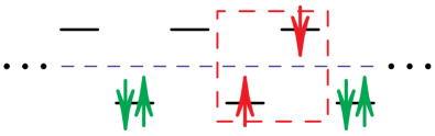
Figure 1: Schematic representation of excitations of the ionic Hubbard model in the band insulator phase. In the absence of hopping terms, the ground state for $U<\delta$ is characterized by occupied odd sites and empty even sites. A pair of excitations appears when an electron hops from an odd to an even site.

In order to unify all electron and hole operators, we define the fermionic operator

$$f_{i,\sigma}=\begin{cases}c^{\phantom{\dagger}}_{i,\sigma}&{\rm for}\leavevmode\nobreak\ i\in{\rm even}\\ h^{\phantom{\dagger}}_{i,\sigma}&{\rm for}\leavevmode\nobreak\ i\in{\rm odd}\end{cases}.$$ (14)

According to these definitions the Hamiltonian (1) reads

$$H=\frac{U\!-\!2\delta}{4}\sum_{i}\mathds{1} + \frac{\delta-U}{2}\sum_{i,\sigma}f^{\dagger}_{i,\sigma}f_{i,\sigma}^{\phantom{\dagger}}$$ (15)

$$+ U\sum_{i}f^{\dagger}_{i,\uparrow}f^{\dagger}_{i,\downarrow}f_{i,\downarrow}^{\phantom{\dagger}}f_{i,\uparrow}^{\phantom{\dagger}}$$

$$+ t\sum_{i,\sigma}(-1)^{i}(f^{\dagger}_{i,\sigma}f^{\dagger}_{i+1,\sigma}+{\rm h.c.}),$$

it still has two sites per unit cell as the original Hamiltonian (1).

It is possible to restore full translational symmetry by applying a suitable local transformation on the fermionic operators

$$f^{\dagger}_{j,\sigma}\longrightarrow e^{-i\frac{\pi}{4}}e^{i\frac{\pi}{2}j}f^{\dagger}_{j,\sigma}.$$ (16)

This transformation leaves the first three terms in Eq. (15) unchanged and eliminates the prefactor $(-1)^{i}$ from the last term. Thereby, we reach

$$H=\frac{U\!-\!2\delta}{4}\sum_{i}\mathds{1} + \frac{\delta-U}{2}\sum_{i,\sigma}f^{\dagger}_{i,\sigma}f_{i,\sigma}^{\phantom{\dagger}}$$ (17)

$$+ U\sum_{i}f^{\dagger}_{i,\uparrow}f^{\dagger}_{i,\downarrow}f_{i,\downarrow}^{\phantom{\dagger}}f_{i,\uparrow}^{\phantom{\dagger}}$$

$$+ t\sum_{i,\sigma}(f^{\dagger}_{i,\sigma}f^{\dagger}_{i+1,\sigma}+{\rm h.c.}).$$

The last term of this Hamiltonian is a Bogoliubov term which creates and annihilates a pair of QPs (originally an electron and a hole) with total spin zero on neighboring sites. In the following, the deepCUT method will be applied to this Hamiltonian.

The conservation of the original electron number in the representation (17) is not manifest. Thus we write down the operator of the total electron number $\widehat{N}$ in terms of $f$-operators

$$\widehat{N}:=\sum_{i,\sigma}c^{\dagger}_{i,\sigma}c^{\phantom{\dagger}}_{i,\sigma}=L+\sum_{i,\sigma}(-1)^{i}f^{\dagger}_{i,\sigma}f^{\phantom{\dagger}}_{i,\sigma},$$ (18)

where $L$ is the number of sites in the chain. The difference between the number of QPs on even sites and on odd sites is a constant of motion. Thus they are always created or annihilated in pairs with an odd distance between them.

III.2 Low-Energy Effective Hamiltonian

The interesting physics of the IHM happens at large values of the Hubbard interaction $U$ approaching the first transition at $U_{c1}$. We focus on the case $U,\delta\gg t$ where the states with finite number of double occupancies (DOs) lie very high in energy. Thus the low-energy physics of the Hamiltonian (17) is governed by the Hilbert subspace without DO. But the subspaces with and without DOs are linked by the Bogoliubov term.

In a first step, we decouple the low- and the high-energy parts of the Hilbert space. The same idea was first realized by Stein perturbatively for the Hubbard model on the square lattice Stein (1997). Extended calculations using self-similar CUTs (sCUT) were carried out at and away from half-filling Reischl et al. (2004); Hamerla et al. (2010) to investigate the range of validity of the mapping from the Hubbard model to the $t$-$J$ model. High-order perturbative calculations for the Hubbard model on the triangular lattice at half-filling have been performed by Yang and co-workers Yang et al. (2010).

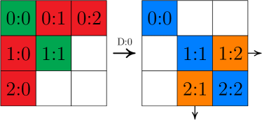
Figure 2: (Color online) Schematic representation of the application of the generator $D\!:\!0$ to the initial Hamiltonian (22). Each part $H_{i:j}$ of the Hamiltonian is depicted by a block; the notation $i\!:\!j$ stands for the number of DOs which is first annihilated ($j$) and then created ($i$). The blank blocks indicate the absence of the correspond interaction in the Hamiltonian. In the final effective Hamiltonian the sector with zero number of DOs is decoupled and the coefficients in other blocks are renormalized as indicated by the change of color/shading.

In the fermionic representation (17) of the IHM it is not evident how many DOs are created or annihilated by a term because this depends on the state to which the terms are applied. Thus, we introduce a representation (Hubbard operators Hubbard (1964)) of hard-core particles defined by

$$g^{\dagger}_{i,\sigma} := \mathinner{|{\sigma}\rangle}_{i}\prescript{}{i}{\mathinner{\langle{0}|}}=(1-n_{i,\bar{\sigma}})f^{\dagger}_{i,\sigma}$$ (19a)

$$g^{\dagger}_{i,d} := \mathinner{|{\uparrow\downarrow}\rangle}_{i}\prescript{}{i}{\mathinner{\langle{0}|}}=f^{\dagger}_{i,\uparrow}f^{\dagger}_{i,\downarrow}$$ (19b)

where $\bar{\sigma}=-\sigma$. The fermionic hard-core operator $g^{\dagger}_{i,\sigma}$ creates a fermion with spin $\sigma$ at site $i$ from the vacuum and the bosonic operator $g^{\dagger}_{i,d}$ creates a DO at site $i$ from the vacuum. They obey the hard-core (anti-)commutation relation

$$\left[g^{\phantom{\dagger}}_{i,\alpha},g^{\dagger}_{j,\beta}\right]_{\pm}=\delta_{i,j}\left(\delta_{\alpha,\beta}\pm g^{\dagger}_{i,\beta}g^{\phantom{\dagger}}_{i,\alpha}\!-\delta_{\alpha,\beta}\!\!\!\sum_{\gamma=\uparrow,\downarrow,d}\!\!\!g^{\dagger}_{i,\gamma}g^{\phantom{\dagger}}_{j,\gamma}\right)$$ (20)

where the anticommutation $[\leavevmode\nobreak\ ,\leavevmode\nobreak\ ]_{+}$ is to be used if both operators are fermionic, otherwise the commutation $[\leavevmode\nobreak\ ,\leavevmode\nobreak\ ]_{-}$ is to be used. The above representation can be reversed to express the $f$-operators in terms of the $g$-operators

$$f^{\dagger}_{i,\sigma}=g^{\dagger}_{i,\sigma}+{\rm sign}(\sigma)g^{\dagger}_{i,d}\leavevmode\nobreak\ g^{\phantom{\dagger}}_{i,\bar{\sigma}}.$$ (21)

The IHM (17) in terms of the $g$-operators can be split into different parts which create and annihilate a specific number of DOs. Explicitly one has

$$H=H_{0:0}+H_{1:1}+H_{1:0}+H_{0:1}+H_{2:0}+H_{0:2},$$ (22)

where $H_{i:j}$ creates $i$ and annihilates $j$ DOs. These parts are given by

$$H_{0:0} = \frac{U\!-\!2\delta}{4}\sum_{i}\mathds{1}+\frac{\delta\!-\!U}{2}\sum_{i,\sigma}g^{\dagger}_{i,\sigma}g_{i,\sigma}^{\phantom{\dagger}}$$ (23a)

$$+t\sum_{i,\sigma}(g^{\dagger}_{i,\sigma}g^{\dagger}_{i+1,\sigma}+{\rm h.c.}),$$

$$H_{1:1} = \delta\sum_{i}g^{\dagger}_{i,d}g_{i,d}^{\phantom{\dagger}},$$ (23b)

$$H_{1:0} = t\sum_{i,\sigma}{\rm sign}(\sigma)(g^{\dagger}_{i,d}g_{i,\bar{\sigma}}^{\phantom{\dagger}}g^{\dagger}_{i+1,\sigma}+g^{\dagger}_{i,\sigma}g^{\dagger}_{i+1,d}g_{i+1,\bar{\sigma}}^{\phantom{\dagger}})$$ (23c)

$$=(H_{0:1})^{\dagger},$$

$$H_{2:0} = t\sum_{i,\sigma}g^{\dagger}_{i,d}g_{i,{\sigma}}^{\phantom{\dagger}}g^{\dagger}_{i+1,d}g_{i+1,{\sigma}}^{\phantom{\dagger}}=(H_{0:2})^{\dagger}.$$ (23d)

These expressions indicate that for $U\approx\delta\gg t$, the low-energy physics takes place in the subspace without DOs. The reduced generator $\eta_{D:0}$ is applied to (22) to disentangle the subspace without any DOs from the remaining Hilbert space. The process is schematically shown in Fig. 2. The final low-energy effective Hamiltonian acts on a three-dimensional local Hilbert space (no fermion present or an $\uparrow$ or $\downarrow$ fermion is present). The fermionic hard-core QP can hop and they interact with one another. In table 1, the relevant monomials $A_{j}$ up to the minimal order $O_{\rm min}\leq 2$ are given. The expression “minimal order” refers to the lowest power in the expansion parameter $x$ in which this term appears. Together with the prefactors $h_{j}(\infty)$ the monomials define the low-energy effective Hamiltonian after the first CUT

$$H^{\rm eff}_{0:0}=\sum_{j=0}h_{j}(\infty)A_{j}.$$ (24)

$j\hskip 28.45274pt$	$A_{j}$	$\hskip 28.45274ptO_{\rm min}$
$0\hskip 28.45274pt$	$\sum\limits_{i}\mathds{1}$	$\hskip 28.45274pt0$
$1\hskip 28.45274pt$	$\sum\limits_{i,\sigma}g^{\dagger}_{i,\sigma}g_{i,\sigma}^{\phantom{\dagger}}$	$\hskip 28.45274pt0$
$2\hskip 28.45274pt$	$\sum\limits_{i,\sigma}\left(g^{\dagger}_{i,\sigma}g_{i+1,\sigma}^{\dagger}+{\rm h.c.}\right)$	$\hskip 28.45274pt1$
$3\hskip 28.45274pt$	$\sum\limits_{i,\sigma}g^{\dagger}_{i,\sigma}g_{i,\sigma}^{\phantom{\dagger}}g^{\dagger}_{i+1,\sigma}g_{i+1,\sigma}^{\phantom{\dagger}}$	$\hskip 28.45274pt2$
$4\hskip 28.45274pt$	$\sum\limits_{i,\sigma}g^{\dagger}_{i,\sigma}g_{i,\sigma}^{\phantom{\dagger}}g^{\dagger}_{i+1,\bar{\sigma}}g_{i+1,\bar{\sigma}}^{\phantom{\dagger}}$	$\hskip 28.45274pt2$
$5\hskip 28.45274pt$	$\sum\limits_{i,\sigma}g^{\dagger}_{i,\sigma}g_{i,\bar{\sigma}}^{\phantom{\dagger}}g^{\dagger}_{i+1,\sigma}g_{i+1,\bar{\sigma}}^{\phantom{\dagger}}$	$\hskip 28.45274pt2$
$6\hskip 28.45274pt$	$\sum\limits_{i,\sigma}\left(g^{\dagger}_{i,\sigma}g_{i+1,\bar{\sigma}}^{\dagger}g^{\phantom{\dagger}}_{i+1,\bar{\sigma}}g_{i+2,\sigma}^{\phantom{\dagger}}+{\rm h.c.}\right)$	$\hskip 28.45274pt2$
$7\hskip 28.45274pt$	$\sum\limits_{i,\sigma}\left(g^{\dagger}_{i,\sigma}g_{i+1,\sigma}^{\dagger}g^{\phantom{\dagger}}_{i+1,\bar{\sigma}}g_{i+2,\bar{\sigma}}^{\phantom{\dagger}}+{\rm h.c.}\right)$	$\hskip 28.45274pt2$

Table 1: The operators $A_{j}$ up to the minimal order $O_{\rm min}=2$ present in the low-energy effective Hamiltonian (24). Note that we combined certain monomials which must have the same prefactor due to symmetries or hermitian conjugation.

In order to verify the convergence of the results, the prefactors of the monomials $A_{1}$, $A_{2}$, and $A_{3}$ are plotted versus $U$ in panels (a), (b), and (c) of Fig. 3, respectively. In each panel, the results for the hopping parameters $t=0.05$ (solid line), $t=0.10$ (dashed line), and $t=0.20$ (dotted-dashed line) in three different orders $2$ (green/light gray), $4$ (blue/dark gray), and $6$ (red/gray) are depicted. For $t=0.05$ the results in the different orders agree nicely for all the three prefactors. Fig. 3 also shows that for $t=0.10$, order $4$ and $6$ still coincide. But for $t=0.20$ we need to go to higher orders to obtain the effective Hamiltonian quantitatively. In the following, we fix the order of deepCUT in this first step to $4$ in the hopping parameter $t$. This appears to be sufficient as long as we focus on low values of $t$ in the following.

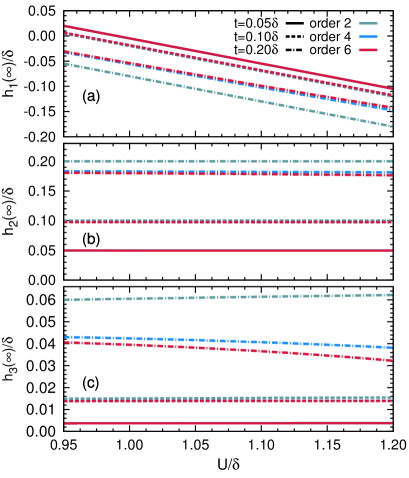
Figure 3: (Color online) The coefficiens $h_{1}(\infty)/\delta$ (a), $h_{2}(\infty)/\delta$ (b), and $h_{3}(\infty)/\delta$ (c) defined in Eq. (24) plotted versus the Hubbard interaction $U/\delta$. The results are obtained by applying the $D\!:\!0$ generator to the Hamiltonian (23). Each panel includes the results for the hopping parameters $t=0.05\delta$ (solid line), $t=0.10\delta$ (dashed line), and $t=0.20\delta$ (dotted-dashed line) in three diferent orders $2$ (green/light gray), $4$ (blue/dark gray), and $6$ (red/gray).

The underlying idea to eliminate processes changing the number of DOs is similar to the one used in the well-known derivation of the $t$-$J$ model from the Hubbard model Hirsch (1985); Fazekas (1999). We stress that the obtained effective Hamiltonian is a renormalized one and that can be systematically improved by including higher orders in $t/\delta$, see also Refs. Reischl et al., 2004; Hamerla et al., 2010; Yang et al., 2010. In Ref. Tincani et al., 2009, Tincani et al. investigated the IHM by restricting the local Hilbert space to the three states. They deal directly with the Hamiltonian (23a) omitting the other processes completely. Their findings for the transition points tend towards the results of the IHM in the limit $U,\delta\gg t$ Tincani et al. (2009).

III.3 The One-Quasiparticle Sector

The effective Hamiltonian derived in the previous subsection is still complicated. It includes various interactions between different QP sectors. These QPs are created and annihilated by the $g$-operators of spin $\uparrow$ and $\downarrow$. To determine the dispersion of a single quasiparticle (1QP), we need to decouple at least the zero- and one-QP sectors from the sectors with more QPs. The reduced generator $\eta_{g:1}$ is required for this goal. Various symmetries and simplification rules are used in order to decrease the runtime and the memory requirement in the deepCUT algorithm so that the high orders can be reached.

We use the symmetries of reflection, the rotation about the $z$-axis of the spins, and the self-adjointness of the Hamiltonian to reduce the number of representative terms by about a factor $8$. The various simplification rules we use are analogous to those introduced in the first paper on deepCUT Krull et al. (2012). In addition, we exploit the conservation of the particle number for each spin separately. For details about the implementation of the simplification rules we refer the reader to the Appendix A. In this way, we were able to reach order $20$ in the hopping parameter $t$ in the calculations for the 1QP dispersion. Up to this order no divergence in the numeric evaluation of the flow equations occurred in the investigated parameter regime.

The final effective Hamiltonian is translationally invariant so that the one-QP sector is diagonalized by a Fourier transformation. The resulting one-QP dispersion reads

$$\omega(k)=h_{0}+2\sum_{d=1}^{n}h_{2n}\cos(2nk)$$ (25)

where the prefactors $h_{d}$ is the hopping element from site $i$ to $i\pm d$. Only hopping elements over even distances occur because odd hops would violate the conservation of the total particle number of original particles, see Eq. (18). All bilinear terms acting on odd distances are of Bogoliubov type.

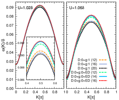
Figure 4: (Color online) The one-QP dispersion of the IHM for $t=0.05\delta$ and $U=1.02\delta$ (left panel) and $U=1.06\delta$ (right panel). The one-QP dispersion is obtained by a successive application of the generators $D\!:\!0$ and $g\!:\!1$, denoted by $D\!:\!0\!+\!g\!:\!1$. The order in $D\!:\!0$ step is fixed to $4$ and the step $g\!:\!1$ is realized in order $12$ (dotted-dashed line), $16$ (solid line), and $20$ (dashed line). The deviations between different orders are maximum close to $K=\frac{\pi}{2}$. In addition, the dispersion resulting from the combination of the deepCUT with ED, denoted $D\!:\!0\!+\!g\!:\!0\!+\!{\rm ED}$, see also main text below, is depicted. The largest deviation between the two approaches occurs around $K=\frac{\pi}{2}$, i.e., at the maximum value of the dispersion.

The one-QP dispersion (25) resulting from the consecutive application of the generators $D\!:\!0$ and $g\!:\!1$, denoted by $D\!:\!0+g\!:\!1$, is depicted in Fig. 4. The shorthand $D\!:\!0+g\!:\!1$ stand for a first application by applying the generator $\eta_{D:0}$. Then, the resulting effective Hamiltonian is block-diagonalized by applying the generator $\eta_{g:1}$. The left panel of Fig. 4 is for $U=1.02\delta$ and the right panel is for $U=1.06\delta$. The hopping prefactor $t$ in Eq. (17) is fixed to $0.05\delta$. The one-QP dispersion is presented for order $12$ (dotted-dashed line), $16$ (solid line), and $20$ (dashed line) in the hopping prefactor $t$.

The left panel in Fig. 4 shows that the results of different orders $12$, $16$, and $20$ accurately coincide in the whole range of momenta $0\leq K<\pi$ demonstrating a good convergence of the deepCUT method. The largest deviation occurs around the momentum $K=\frac{\pi}{2}$ where the dispersion is maximum as is shown in the inset.

But the convergence for increasing order is worse for $U=1.06\delta$ because we approach the transition point, $U_{c}\approx 1.07\delta$. Again, the largest deviation between different orders occurs near the total momentum $K=\frac{\pi}{2}$. The one-QP dispersion $\omega(k)$ shows a tendency to decrease on increasing the order of calculations.

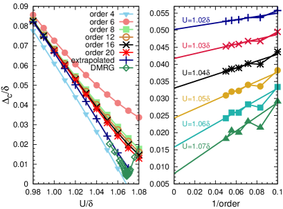
Figure 5: (Color online) The charge gap of the ionic Hubbard model for the hopping parameter $t=0.05\delta$. Left panel: The charge gap as a function of $U/\delta$ in various orders. The deepCUT results extrapolated to infinite order are also depicted. The extrapolated DMRG results Manmana et al. (2004) are shown for comparison. The deviation in our analysis at finite orders becomes large close to the transition point, $U_{c}=1.07\delta$. The difference between extrapolated deepCUT results and DMRG results is about $0.002\delta$. Right panel: The charge gap versus the inverse of the order for different values of Hubbard interaction $U$. The deepCUT results are extrapolated to infinite order by a linear fit to the last four points in $1/{\rm order}$.

The charge gap ($\Delta_{c}$) is defined as the energy necessary to add an electron plus the energy for taking an electron from the system

$$\Delta_{c}=E_{0}(N+1)+E_{0}(N-1)-2E_{0}(N),$$ (26)

where $E_{0}(N)$ is the ground state energy of the system with $N$ particles. For our electron-hole symmetric Hamiltonian (1), it is twice the minimum of the dispersion $\Delta_{c}=2\omega_{\rm min}$.

Besides the charge gap, the following gaps are relevant in the IHM as well. The exciton gap $\Delta_{e}$ is defined as the first excitation energy in the sector with the same particle number as in the ground state and with total spin zero

$$\Delta_{e}:=E_{1}(N,S=0)-E_{0}(N,S=0),$$ (27)

where $E_{1}$ stands for the first excited state in the corresponding sector. Similarly, the spin gap is defined as the first excitation energy in the sector with the same particle number, but with total spin one

$$\Delta_{s}:=E_{1}(N,S=1)-E_{0}(N,S=0).$$ (28)

In our formalism, the exciton gap is given by the lowest energy of the first singlet bound state and the spin gap by the first triplet bound state, if binding occurs. Otherwise, the lowest scattering states matter. Excited states of two QPs will be considered in detail below in Sect. III.4.

The charge gap for different orders of the hopping prefactor $t$ is plotted in the left panel of Fig. 5 as function of Hubbard interaction $U$. The deepCUT results extrapolated to infinite order by a linear fit in $1/{\rm order}$ are also depicted. The DMRG results, rescaled to the present units, are shown for comparison Manmana et al. (2004). Data is given up to $U=1.08\delta$ because around this point the phase transition to the SDI takes place (see the next subsection) and the QP picture breaks down. Fig. 5 shows that the results of the deepCUT at high orders coincide very well for $U<1.00\delta$. For $U>1.00\delta$, however, especially close to the transition point, the different orders separate due to the numerical deviations indicating a poorer convergence. The difference between the extrapolated deepCUT results and the DMRG results is about $0.002\delta$. We draw the reader’s attention to the accuracy of such data. The energy scale of the initial model before the renormalizing unitary transformations is $U+\delta\approx 2\delta$ so that the transformations are still precise on energy scales reduced by three orders of magnitude.

In the right panel of Fig. 5, the charge gap versus the inverse order is displayed for various values of $U$. The charge gap decreases on increasing order. The deepCUT results are extrapolated to infinite order by a linear fit to the last four points. This plot illustrates how the deepCUT calculations converge as function of the order in the hopping $t$. The deepCUT method as used in the present work is a renormalizing approach based on a truncation in real space. This means that processes are tracked only up to a certain range in real space. This range is determined by the order of the calculations interpreted as the maximum number of hops on the lattice. Thus it is clear that the approach as presented here runs into difficulties upon approaching continuous phase transitions where long-range processes become essential.

III.4 The Two-Quasiparticle Sector

In the framework of deepCUT, the treatment of sectors with higher number of QPs is also possible Knetter and Uhrig (2000); Windt et al. (2001); Knetter et al. (2001, 2003a); SCHMIDT and UHRIG (2005); Fischer et al. (2010); Krull et al. (2012). The two-QP sector can be decoupled by using the reduced generator $\eta_{g:2}$. This generator will yield an effective Hamiltonian that can be diagonalized for each combination of the total momentum $K$, total spin $S$, and total magnetic quantum number $M$. The two-QP states with fixed $K$, $S$, and $M$ read

$$\mathinner{|{K;d}\rangle}^{S,M}\!\! = \sum_{\sigma_{1}\sigma_{2}}A^{S,M}_{\sigma_{1},\sigma_{2}}\mathinner{|{K,\sigma_{1};d,\sigma_{2}}\rangle}$$

$$= \frac{1}{\sqrt{L}}\sum_{r}e^{iK(r+\frac{d}{2})}\sum_{\sigma_{1}\sigma_{2}}A^{S,M}_{\sigma_{1},\sigma_{2}}\mathinner{|{r,\sigma_{1};r+d,\sigma_{2}}\rangle},$$

where $\sigma_{1}$ and $\sigma_{2}$ indicate the spins of the QPs, $A^{S,M}_{\sigma_{1},\sigma_{2}}$ are the appropriate Clebsch-Gordon coefficients, $L$ is the system size, i.e, the number of sites. The sum runs over all lattice sites and $d>0$ is the distance between the two QPs which cannot be zero due to the hard-core property. Furthermore, because the two constituting fermions are indistinguishable after the particle-hole transformation, the Clebsch-Gordon coefficients take the contributions with negative $d$ into account.

The Hamiltonian matrix in the two-QP sector is composed of three different submatrices refering to different total charge. Both QPs can be original electrons, or holes, or one is an electron and the other a hole. Here we refer to the fermions before the particle-hole transformations. If the two-QP state (LABEL:eq:2qp_state) contains only odd distances $d$ it consists of an electron and a hole. But if the two-QP state is made of two original electrons or two holes, the distances between them are even, cf. Eq. (18). Here we focus on the case of two-QP states with one electron and one hole and discuss the possible triplet and singlet bound states.

The sector with two holes (or two electrons) is also very interesting in the context of superconductivity. A recent investigation of the IHM including next-nearest neighbor (NNN) hopping terms on the honeycomb lattice found evidence for superconducting behavior upon hole doping Watanabe and Ishihara (2013). A dynamic mean field theory study of the model also indicates an interesting half-metallic behavior on doping away from half-filling Garg et al. (2013). But these issues are beyond the scope of present article.

The Hamiltonian matrix can be constructed by applying the Hamiltonian parts $H_{1:1}$ and $H_{2:2}$ to the state $\mathinner{|{K,\sigma_{1};d,\sigma_{2}}\rangle}$. For $H_{1:1}$, we obtain

$$H_{1:1} \mathinner{|{K,\sigma_{1};d,\sigma_{2}}\rangle}=$$ (30)

$$+\sum_{n>-d}\sum_{\beta_{1}}e^{iK\frac{n}{2}}\prescript{\beta_{1}\!\!}{\sigma_{1}\!\!}{\Big{[}}{\mathcal{C}_{1}^{1}\Big{]}}^{\!n}\mathinner{|{K,\beta_{1};+d+n,\sigma_{2}}\rangle}$$

$$-\sum_{n<-d}\sum_{\beta_{1}}e^{iK\frac{n}{2}}\prescript{\beta_{1}\!\!}{\sigma_{1}\!\!}{\Big{[}}{\mathcal{C}_{1}^{1}}{\Big{]}}^{\!n}\mathinner{|{K,\sigma_{2};-d-n,\beta_{1}}\rangle}$$

$$+\sum_{n<d}\sum_{\beta_{2}}e^{iK\frac{n}{2}}\prescript{\beta_{2}\!\!}{\sigma_{2}\!\!}{\Big{[}}{\mathcal{C}_{1}^{1}}{\Big{]}}^{\!n}\mathinner{|{K,\sigma_{1};+d-n,\beta_{2}}\rangle}$$

$$-\sum_{n>d}\sum_{\beta_{2}}e^{iK\frac{n}{2}}\prescript{\beta_{2}\!\!}{\sigma_{2}\!\!}{\Big{[}}{\mathcal{C}_{1}^{1}}{\Big{]}}^{\!n}\mathinner{|{K,\beta_{2};-d+n,\sigma_{1}}\rangle},$$

where the appearance of the minus signs is due to the fermionic nature of the problem. We use the shorthand

$$\prescript{\beta\!\!}{\sigma\!\!}{\Big{[}}{\mathcal{C}_{1}^{1}}{\Big{]}}^{\!n}:=\mathinner{\langle{r\!-\!n,\beta}|}H_{1:1}\mathinner{|{r,\sigma}\rangle}.$$ (31)

Similarly, for $H_{2:2}$ we have

$$H_{2:2} \mathinner{|{K,\sigma_{1};d,\sigma_{2}}\rangle}=$$

$$-\sum_{n}\sum_{d^{\prime}>0}\sum_{\beta_{1}\beta_{2}}e^{iK\left(n+\frac{d-d^{\prime}}{2}\right)}\prescript{\beta_{1}\!\beta_{2}\!\!}{\sigma_{1}\!\sigma_{2}\!\!}{\Big{[}}{\mathcal{C}_{2}^{2}}{\Big{]}}^{\!nd^{\prime}}_{d}\mathinner{|{K,\beta_{1};d^{\prime},\beta_{2}}\rangle},$$

with the definition

$$\prescript{\beta_{1}\!\beta_{2}\!\!}{\sigma_{1}\!\sigma_{2}\!\!}{\Big{[}}{\mathcal{C}_{2}^{2}}{\Big{]}}^{\!nd^{\prime}}_{d}\!\!:=\!\mathinner{\langle{r\!-\!n,\beta_{1};r\!-\!n\!+\!d^{\prime},\beta_{2}}|}H_{2:2}\mathinner{|{r,\sigma_{1};r+d,\sigma_{2}}\rangle}.$$ (33)

In order to fix the fermionic sign in the definition (33) uniquely we assume from now on that in each monomial of $H_{2:2}$ the creation operators are placed in front of the annihilation operators and the annihilation and the creation parts are separately site-ordered.

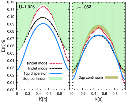
Figure 6: (Color online) Low-lying excitation spectrum including one-quasiparticle dispersion (solid line), two-quasiparticle and three-quasiparticle continuum (colored/shaded regions), singlet (dashed line) and triplet (dotted-dashed line) bound states. The results are obtained by consecutive application of the generators $D\!:\!0$ and $g\!:\!2$. The order of the transformation for $D\!:\!0$ is $4$ and for $g\!:\!2$ it is $12$ which is the highest converging order. The hopping element is $t=0.05\delta$. The Hubbard interaction $U$ is fixed to $1.02\delta$ for the left panel and to $U=1.06\delta$ for the right panel. There are two singlet bound states near the total momentum $K=\pi$ and around $K=\frac{\pi}{2}$. The triplet bound state is almost symmetric around $K=\frac{\pi}{2}$ and exists in the whole BZ. For $U=1.06\delta$, the two-quasiparticle continuum lies completely within the three-quasiparticle continuum.

The low-lying excitation spectra for $U=1.02\delta$ and $U=1.06\delta$ are depicted in the left and in the right panel of Fig. 6, respectively. The hopping $t$ is fixed to $0.05\delta$. The order of the second CUT is $12$. We cannot go beyond this order because the flow equations for the two-QP sector do not converge in higher orders. As can be seen in the right panel, the two-QP continuum lies within the three-QP continuum. The lower edge of the four-QP continuum (not shown) lies also close in energy to the lower edge of two-QP continuum. This large overlap between continua of different number of QPs is the major reason of divergence of the flow equations Fischer et al. (2010).

For both values of $U$ in Fig. 6 there are two singlet and one triplet bound states. The singlet bound modes occur only near the total momentum $K=\pi$ and around $K=\frac{\pi}{2}$. The triplet bound mode becomes more and more symmetric about $K=\frac{\pi}{2}$ as the Hubbard interaction $U$ is increased and approaches the transition point $U_{c1}\sim 1.07\delta$. We attribute the wiggling of the singlet mode for $U=1.06\delta$ around the total momentum $K=\frac{\pi}{2}$ to the truncation of the flow equations. For $U=1.06\delta$, the lowest excited state is the singlet bound state that appears at the total momentum $K=\pi$. This mode becomes soft, i.e, its energy vanishes, upon increasing the Hubbard interaction further indicating the first phase transition at $U_{c1}$ from the BI to the SDI phase.

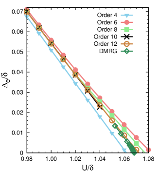
Figure 7: (Color online) The exciton (or singlet) gap $\Delta_{e}$ versus the Hubbard interaction in various orders. The hopping is fixed to $t=0.05\delta$. The exciton gap at becomes soft for $U_{c}=1.072\delta$ in order $12$. For comparison, the DMRG prediction of the first transition is $U_{c}=1.069\delta$ Manmana et al. (2004).

The exciton gap is plotted versus the interaction $U$ in Fig. 7 for different orders. Due to divergence of the flow equations no values are reported in order $10$ for $U>1.04\delta$. For the same reason, orders higher than $12$ were not accessible. The extrapolated DMRG results extracted from Ref. Manmana et al., 2004 and rescaled to the present units are also shown. The deepCUT results at high orders are very close to the DMRG results. The DMRG prediction of the transition point is $1.069\delta$. In our analysis in order $12$ the exciton gap vanishes at $U_{c}=1.072\delta$. The deepCUT results for the exciton gap $\Delta_{e}$ converge better upon increasing order than the deepCUT results for the charge gap $\Delta_{c}$ shown in Fig. 5. We attribute this to the larger separation in energy from the closest continuum.

We studied the energy difference between the spin and the charge gap. While this difference is finite in any finite order, its extrapolation in the inverse order is consistent with a zero difference in the BI phase, i.e., for $U\leq U_{c1}$. In view of the definitions (27) and (28) this implies that no binding between two QPs occurs in the two-QP sector with total $S=1$. These findings are to be compared to previous DMRG data. Takada and Kido extrapolated the DMRG results to infinite system size and deduced that the spin gap and charge gap become different before the first transition point $U_{c1}$ Takada and Kido (2001). The equality of spin and charge gaps up to the first transition point is supported by other extrapolated DMRG calculations Manmana et al. (2004); Lou et al. (2003); Kampf et al. (2003).

The deepCUT approach realized in real space, the range of processes taken into account is proportional to the order of the calculation. Thus we expect the deepCUT method to provide accurate results as long as the order is larger than the correlation length $\xi$ in units of the lattice spacing of the system. The correlation length can be estimated as Sørensen and Affleck (1993); Okunishi et al. (2001)

$$\xi\approx\frac{v}{\Delta},$$ (34)

where $v$ is the velocity for vanishing gap and $\Delta$ is the gap present in the system. The relation (34) stems from the assumption that the low-energy physics of the model fulfills an (approximate) Lorentzian symmetry.

In the IHM, the exciton gap is the smallest gap and hence we set $\Delta=\Delta_{e}$. The fermionic velocity can be obtained by fitting $\omega(k)=v\sin(k)$ to the one-QP dispersion. We find $\xi=\frac{0.09}{0.038}\approx 2.4$ for $U=1.02\delta$, $\xi=\frac{0.07}{0.008}\approx 8.8$ for $U=1.06\delta$, and $\xi=\frac{0.07}{0.0015}\approx 47$ for $U=1.07\delta$. The rapid increase of $\xi$ on approaching the transition point $U_{c1}$ reflects the vanishing exciton gap $\Delta_{e}$. This implies that the deepCUT approach parametrized in real space naturally becomes inaccurate on approaching $U_{c1}$.

IV Exact Diagonalization in the Thermodynamic Limit

The deepCUT results close to the transition point is not quantitative, especially for the charge gap for reasons given above. In this section, we aim at improving the results by following the route used previously in Ref. Fischer et al., 2010. The goal of the deepCUT is chosen less ambitious, i.e., less terms are rotated away. This makes the deepCUT step less prone to inaccuracies and convergence can be achieved more easily. But the disadvantage is that the resulting effective Hamiltonian is not yet diagonal or block-diagonal so that the subsequent analysis becomes more demanding. Here we will employ exact diagonalization in restricted subspaces for this purpose.

IV.1 Construction of the Hamiltonian Matrix

In order to take into account processes of longer range for the important excited states, we only decouple the ground state from the subspaces with finite number of QPs. This is achieved by applying the reduced generator $g\!:\!0$. This generator keeps interactions and transitions between different excited states. Because the system under study is fermionic, there are only terms in the Hamiltonian with even number of fermionic operators. Thus there is no process linking one QP and two QPs: $H_{2:1}=0$. Therefore, the major off-diagonal interaction for one-QP states is $H_{3:1}+H_{1:3}$ and for two-QP states it is $H_{4:2}+H_{2:4}$.

After applying the generator $g\!:\!0$, the effective Hamiltonian has the following structure

$$H_{\rm eff} = H_{0:0}+H_{1:1}+H_{2:2}+H_{3:3}+H_{4:4}$$ (35)

$$+(H_{3:1}+{\rm h.c.})+(H_{4:2}+{\rm h.c.})$$

$$+{\rm less\leavevmode\nobreak\ important\leavevmode\nobreak\ terms},$$

where the less important terms include the parts which involve states with more than four QPs. These interactions have much less effect than $H_{3:1}$ and $H_{4:2}$ on the low-energy spectrum given by the eigenvalues in the one-QP and in the two QP sectors.

The effect of off-diagonal interactions between one- and three-QP states and between two- and four-QP states can be considered by restricting the Hilbert space to four-QP states and performing an exact diagonalization (ED) within this restricted Hilbert space. The effect of the Hamiltonian is stored in two separate matrices, one for the states that are built from one and three QPs and the other for the states built from two and four QPs. We stress that also states with four QPs have to be considered to be able to address modifications in the two-QP spectrum.

Because the ground state is decoupled in the deepCUT step, we can work directly in the thermodynamic limit by introducing the states with specific total momentum $K$, total spin $S$, and total magnetic number $M$

$$\mathinner{|{K}\rangle}^{S,M}\! =\!\frac{1}{\sqrt{L}}\sum_{r}e^{iKr}\mathinner{|{r}\rangle}^{S,M},$$ (36a)

$$\mathinner{|{K;d}\rangle}^{S,M}\! =\!\frac{1}{\sqrt{L}}\sum_{r}e^{iK\left(r+\frac{d}{2}\right)}\mathinner{|{r;r\!+\!d}\rangle}^{S,M},$$ (36b)

$$\mathinner{|{K;d_{1};d_{2}}\rangle}^{S,M}_{\alpha}\! =\!\frac{1}{\sqrt{L}}\sum_{r}e^{iK\left(r+\frac{2d_{1}+d_{2}}{3}\right)}\times$$

$$\hskip 22.76228pt\times\mathinner{|{r;r\!+\!d_{1};r\!+\!d_{1}\!+\!d_{2}}\rangle}^{S,M}_{\alpha},$$ (36c)

$$\mathinner{|{K;d_{1};d_{2};d_{3}}\rangle}^{S,M}_{\alpha}\! =\!\frac{1}{\sqrt{L}}\sum_{r}e^{iK\left(r+\frac{3d_{1}+2d_{2}+d_{3}}{4}\right)}\times$$

$$\times\mathinner{|{r;r\!+\!d_{1};r\!+\!d_{1}\!+\!d_{2};r\!+\!d_{1}\!+\!d_{2}\!+\!d_{3}}\rangle}^{S,M}_{\alpha},$$ (36d)

where $d_{1}$, $d_{2}$, and $d_{3}$ are the distances between the QPs, and $\alpha$ is an additional quantum number that specifies the spin configuration. The quantum number $\alpha$ is required for distinction because there is more than one spin configuration with three and four QPs for given total spin and total $S_{z}$.

The Hamiltonian matrix is constructed for each fixed set of $K$, $S$, and $M$. The action of the parts of the Hamiltonian $H_{i:j}$ for $i,j\leq 4$ on the states (36) is calculated analytically. The effect of $H_{1:1}$ and $H_{2:2}$ on the two-QP state is already reported in Eqs. (30) and (LABEL:eq:H22_on_2qp). The effect of $H_{1:1}$ on two-QP state has $4$ contributions while it has $9$ and $16$ contributions for three- and four-QP states, respectively. The application of $H_{2:2}$ on three- and four-QP states lead to $9$ and $36$ different contributions. The numbers of contributions can be understood easily. For instance, $H_{1:1}$ has three different possibilities to annihilate a QP when it acts on a three-QP state and it can also create a QP in three distinct positions, namely to the left, between, and to the right of the two QPs on the chain, leading to $9$ contributions. The process is schematically shown in Fig. 8.

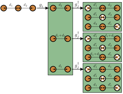
Figure 8: (Color online) Schematic representation of the application of $H_{1:1}=\sum_{i,j}t_{i,j}g_{i}^{\dagger}g_{j}^{\phantom{\dagger}}$ on the three-QP state $\mathinner{|{K;d_{1};d_{2}}\rangle}$ defined in (36c). There are three different possibilities for the operator $g_{j}^{\phantom{\dagger}}$ to annihilate a QP and the operator $g_{i}^{\dagger}$ can create a QP in three distinct positions: to the left, between, and to the right of the two QPs already present. This leads to $9$ different contributions.

The explicit expressions for the action of different parts of the Hamiltonian (35) on the states (36) are calculated and reported in the supplementary electronic material. These expressions are general and can be used for all hardcore fermionic or bosonic problems. The two-, three-, and four-QP states with total spin $S=0$ and $S=1$, total magnetic number $M=0$ and $M=1$, and the additional label $\alpha$ are also given in the supplementary electronic part.

The idea that we have applied here is similar to what had been introduced in Ref. Fischer et al., 2010 to describe QP decay with CUT. The main difference is that we have to take care of the fermionic minus sign and to consider also the states with four QPs. Including the four-QP states not only leads to large analytic expressions, but also limits the maximum relative distances that can be treated numerically. For the following results, the Hamiltonian matrix has been constructed with maximum distances $d_{1}^{\rm max}=d_{2}^{\rm max}=d_{3}^{\rm max}=24$.

IV.2 Low-lying Excitation Spectrum

The charge and exciton gaps obtained by the combination of deepCUT and ED are depicted in Fig. 9. We denote this approach by $D\!:\!0+g\!:\!0+{\rm ED}$ which means that the effective Hamiltonian is derived by the consecutive application of the generators $\eta_{D:0}$ and $\eta_{g:0}$. Then this effective Hamiltonian is analyzed by ED method as described above. Due to the restriction of the Hilbert space in the ED, its results overestimate the eigen values of the effective Hamiltonian, i.e., they provide upper bounds to them. But note that the effective Hamiltonian has only a limited accuracy due to the truncations in the course of the deepCUT $D\!:\!0+g\!:\!0$ so that the ED results cannot be taken as rigorous upper bounds. If we, however, assume that the inaccuracies introduced in the derivation of the effective Hamiltonian are of minor importance, the ED results can be taken as an upper bound for the correct eigen values.

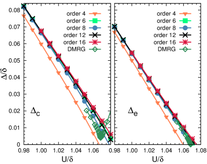
Figure 9: (Color online) The charge gap (left panel) and the exciton gap (right panel) vs. $U$ obtained by $D\!:\!0\!+\!g\!:\!0\!+\!{\rm ED}$, see main text. The order of the $D\!:\!0$ step is $4$ and $g\!:\!0$ is carried out in various orders, see legend. The data for charge gap appears to be more robust in $D\!:\!0\!+\!g\!:\!0\!+\!{\rm ED}$ than in the pure deepCUT analysis $D\!:\!0\!+\!g\!:\!2$.

The left panel of Fig. 9 shows that the difference between the data obtained by $D\!:\!0\!+\!g\!:\!0\!+\!{\rm ED}$ and the DMRG results is smaller than the difference of the data of the pure application of the deepCUT to the DMRG results, cf. Fig. 5. For the charge gap close to the phase transition, the deviation between our results and the DMRG data is decreased from about $1\%$ for the pure deepCUT to about $0.5\%$ for the combination of deepCUT and ED.

In the right panel of Fig. 9, the exciton gap is plotted vs. the Hubbard interaction $U$. The results agree nicely with the DMRG results for all orders higher than $4$. Inspecting the trend of the results for increasing order they appear to converge to values slightly higher than the DMRG results. We attribute this fact to the restriction of the Hilbert space in the ED treatment making it an upper bound.

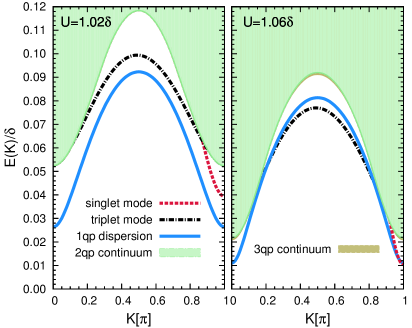
Figure 10: (Color online) The low-energy spectrum of the IHM including one-quasiparticle dispersion (solid line), two- and three-quasiparticle continuum (solid region), and singlet (dashed line) and triplet (dotted-dashed line) bound states. The results are obtained by $D\!:\!0\!+\!g\!:\!0\!+\!{\rm ED}$. The deepCUT steps $D\!:\!0$ and $g\!:\!0$ are performed in orders $4$ and $16$, respectively. For the ED, the Hamiltonian matrix is constructed for maximum relative distances of $24$. The hopping is fixed to $t=0.05\delta$ for both panels; $U=1.02\delta$ in the left panel and $U=1.06\delta$ in the right panel. For $U=1.06\delta$, the lower edge of two- and three-quasiparticle continuum are very close to each other. No singlet bound state is found near the total momentum $K=\pi/2$ in contrast to the pure deepCUT $D\!:\!0\!+\!g\!:\!2$, see Fig. 6.

The one-QP dispersion obtained by the combination $D\!:\!0+g\!:\!0+{\rm ED}$ is plotted in Fig. 4 for the two different values of the Hubbard interaction $U=1.02\delta$ (left panel) and $U=1.06\delta$ (right panel). In this figure, we compare the results of pure deepCUT with the results of the combination of deepCUT and ED. For $U=1.02\delta$, both methods coincide nicely except very close to $K=\frac{\pi}{2}$ where the maximum deviation occurs. Around $K=\frac{\pi}{2}$ the results of deepCUT plus ED lie a bit higher in energy than those by pure deepCUT, see also inset. It is not clear whether the small difference is due to the restriction of the Hilbert space in ED implying a certain overestimation or whether it is due to the effect of long-range processes that are less well captured by the pure deepCUT.

Next, we focus on the right panel of Fig. 4 where $U=1.06\delta$ close to the transition point. Here the difference between the two methods is larger. For the momenta near $0$ and $\pi$ the combination $D\!:\!0+g\!:\!0+{\rm ED}$ yields a dispersion with lower energy while for the momenta around $\frac{\pi}{2}$ the result from $D\!:\!0+g\!:\!2$ is the lower one. From the comparison with the extrapolated DMRG results for the charge gap we deduce that the dispersion of $D\!:\!0+g\!:\!0+{\rm ED}$ is more accurate near $K=0$ and $K=\pi$. Thus we presume that also around $K=\frac{\pi}{2}$ the $D\!:\!0+g\!:\!0+{\rm ED}$ data is more accurate, but there is no data from alternative approaches available to corroborate this conclusion.

Let us turn to Fig. 10 which shows the low-energy spectrum of the IHM obtained by $D\!:\!0+g\!:\!0+{\rm ED}$ with the orders $4$ and $16$ for the deepCUT steps $D\!:\!0$ and $g\!:\!0$, respectively. The left and right panels are again for $U=1.02\delta$ and $U=1.06\delta$. The lower edge of the three-QP continuum for $U=1.06\delta$ lies close to the lower edge of the two-QP continuum. The major difference between this figure and the pure deepCUT results plotted in Fig. 6 is the absence of the singlet bound state around the total momentum $K=\pi/2$. This difference may arise from the restricted relative distances of QPs in the ED treatment. The singlet bound state mode near $K=\pi/2$ has a small binding energy indicating that it is weakly bound and thus extending over large distances. Its extension is restricted due to computational limitations and the binding may be suppressed in the ED spuriously.

V Beyond the Transition Point: A Mean Field Study

The deepCUT approach realized in the previous sections is based on the QPs of the BI, i.e., the more complicated, dressed excitations close to the transition to the SDI are continuously mapped to the simple QPs of the BI. The same quantum numbers are used in analogy to Fermi liquid theory which uses the same quantum numbers as the Fermi gas. As long as the system is located on the BI side of the phase transition, only a few-particle problem remains to be solved in a subsequent step to find the low-lying excitation spectrum. But this QP picture breaks down when a phase transition occurs. Beyond the transition point, a macroscopic number of QPs of the BI condenses forming the new phase. This new phase displays other types of elementary excitations.

Our analysis of the BI of the IHM in the previous sections showed that the exciton gap decreases on increasing the Hubbard interaction and vanishes at a critical value $U_{c1}$. This critical interaction was found to be $U_{c1}=1.072\delta$ for $D\!:\!0+g\!:\!2$ in order $12$, see Fig. 7. How can we proceed beyond the transition and still profit from the effective Hamiltonians obtained by deepCUT? The most systematic way would be to set up a CUT with respect to the ground state and the elementary excitations for $U>U_{c1}$. But there are two obstacles to this route. The first one is that one has to know and to characterize the SDI ground state sufficiently well to be able to set up a CUT. The second one is that this approach would require to implement another, different CUT which is tedious.

Thus we choose a slightly modified approach and continue to use the implemented CUT to derive an effective Hamiltonian by applying $D\!:\!0+g\!:\!2$ and then to analyze this effective Hamiltonian by a perturbative approach. The guiding idea is that the terms driving the phase transition are small and can be treated perturbatively as long as the system is considered close to the phase transition. In this way, one continues to profit from the deepCUT implemented to obtain effective Hamiltonians. We use the deepCUT $D\!:\!0+g\!:\!2$ in order $12$ to derive the effective Hamiltonian that we analyse perturbatively in the sequel. This deepCUT is not yet so sensitive to be spoilt by the instability towards the SDI because the latter takes place on very low energy scales.

For simplicity, we choose here a mean-field approximation as a first step of a perturbative treatment. Although this approach is not able to capture the correct critical behavior in low dimensions and underestimates the role of fluctuations, it provides us with an estimate which phases are lower in energy. Since the exciton becomes soft at $U_{c1}$ the SDI can be seen as a condensate of excitons. The particle-hole transformation that we performed maps the original exciton into a bound state of two fermions, i.e., the exciton appears as Cooper pair. Thus we expect a BCS-type theory to describe the SDI phase transition.

The effective Hamiltonian is represented in terms of hardcore fermions $\{g_{i,\sigma}\}$ and it includes various interactions within and between sectors of different numbers of QPs. In the following, we consider this effective Hamiltonian up to quadrilinear interactions and ignore interaction terms acting on higher numbers of QPs. Hence the effective Hamiltonian takes the general form

$$H_{\rm eff}=H_{0:0}+H_{1:1}+H_{2:2},$$ (37a)

where

$$H_{0:0} = E_{0}\mathds{1},\allowdisplaybreaks[4]$$ (37b)

$$H_{1:1} = \sum_{ij}\Gamma_{j;i}\leavevmode\nobreak\ g^{\dagger}_{j}g^{\phantom{\dagger}}_{i},\allowdisplaybreaks[4]$$ (37c)

$$H_{2:2} = \sum_{ijkl}\Gamma_{kl;ij}\leavevmode\nobreak\ g^{\dagger}_{k}g^{\dagger}_{l}g^{\phantom{\dagger}}_{i}g^{\phantom{\dagger}}_{j}.$$ (37d)

The prefactors $\Gamma_{j;i}$ and $\Gamma_{kl;ij}$ are nonzero up to an interaction range proportional to the order of calculations. The processes of longer range are all zero. Because the effective Hamiltonian (37a) is obtained by applying the reduced generator $g\!:\!2$ no off-diagonal interactions such as $H_{3:1}$ appear.

In order to apply the Wick theorem, we neglect the hardcore property of the operators and treat them like usual fermions. Due to this approximation two fermions with different spin are allowed to occupy the same site. It is also possible to deal with the hardcore property by the slave-particle techniques, see Ref. Vaezi, 2011 and references therein, or by the Brueckner approach Kotov et al. (1998). But such analyses are beyond the scope of present investigation.

For a self-consistent mean-field approximation the symmetries of the ground state are essential. In order to describe the SDI phase of the IHM, we take the possibility of a spontaneous symmetry breaking into account with nonzero anomalous expectation values (see below). The broken symmetry is the parity with respect to reflection about a site. Thus adjacent bonds may become different even though in the original Hamiltonian the (directed) bond from site 0 to 1 was identical to the one from 0 to -1. This is characteristic of the SDI as found in previous studies based on variational quantum Monte Carlo Wilkens and Martin (2001) and DMRG Manmana et al. (2004); Takada and Kido (2001); Lou et al. (2003); Zhang et al. (2003); Kampf et al. (2003); Tincani et al. (2009); Legeza et al. (2006). Thus, we assume for the expectation values

$$\langle g^{\dagger}_{i,\sigma}g^{\dagger}_{i+m,\sigma}\rangle \neq \langle g^{\dagger}_{i+1,\sigma}g^{\dagger}_{i+m+1,\sigma}\rangle\neq 0,$$ (38a)

$$\langle g^{\dagger}_{i,\sigma}g^{\phantom{\dagger}}_{i+n,\sigma}\rangle = \langle g^{\dagger}_{i+1,\sigma}g^{\phantom{\dagger}}_{i+n+1,\sigma}\rangle\neq 0,$$ (38b)

where $m$ and $n$ stand for odd and even distances, respectively. The maximum values of $m$ and $n$ depend on the order in which the deepCUT was performed. All the above expectation values are zero in the BI phase where the ground state is the vacuum of “$g$-particles”, but they become finite as soon as the exciton begins to condense and the phase transition occurs.

For a transparent notation, we express the $g$-operators acting on even and odd sites by $a$- and $b$-operators, respectively. The resulting mean field Hamiltonian takes the BCS-form

$$H_{\rm BCS} = \frac{L}{2}(\epsilon^{A}_{0}+\epsilon^{B}_{0})\allowdisplaybreaks[4]$$ (39)

$$+\sum_{r\in{\rm even},\sigma}\!\!\left(t^{A}_{0}:a^{\dagger}_{r,\sigma}a^{\phantom{\dagger}}_{r,\sigma}:+\sum_{n=2,4,\cdots}\!\!t^{A}_{n}:a^{\dagger}_{r,\sigma}a^{\phantom{\dagger}}_{r+n,\sigma}+{\rm h.c.}:\right)\allowdisplaybreaks[4]$$

$$+\sum_{r\in{\rm odd},\sigma}\!\left(t^{B}_{0}:b^{\dagger}_{r,\sigma}b^{\phantom{\dagger}}_{r,\sigma}:+\sum_{n=2,4,\cdots}\!\!t^{B}_{n}:b^{\dagger}_{r,\sigma}b^{\phantom{\dagger}}_{r+n,\sigma}+{\rm h.c.}:\right)\allowdisplaybreaks[4]$$

$$+\sum_{r\in{\rm even},\sigma}\hskip 2.84544pt\sum_{m=1,3,\cdots}\Delta^{A}_{m}:a^{\dagger}_{r,\sigma}b^{\dagger}_{r+m,\sigma}:+{\rm h.c.}\allowdisplaybreaks[4]$$

$$+\sum_{r\in{\rm odd},\sigma}\hskip 5.69046pt\sum_{m=1,3,\cdots}\Delta^{B}_{m}:b^{\dagger}_{r,\sigma}a^{\dagger}_{r+m,\sigma}:+{\rm h.c.}$$

where we have divided the lattice into the two sublattices $A$ and $B$ of even sites and odd sites, respectively. The prefactors $\epsilon^{A}_{0}$, $\epsilon^{B}_{0}$, $t^{A}_{d}$, $t^{B}_{d}$, $\Delta^{A}_{d}$, and $\Delta^{B}_{d}$ depend on the coefficients of the effective Hamiltonian, which stem from the flow equations, see Eq. (6), and from the expectation values introduced in Eq. (38). Due to the identity (38b), the hopping prefactors of the two sublattices are identical. So we unify them omitting the sublattice index $t^{A}_{d}=t^{B}_{d}=:t_{d}$.

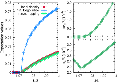
Figure 11: (Color online) Analysis of the effective Hamiltonian obtained by $D:0+g:2$ in order 12 within the BCS-type approximation. The hopping prefactor $t$ is $0.05\delta$. Left panel: Expectation values of the local density, the nearest-neighbor (NN) Bogoliubov term, and the next-nearest-neighbor (NNN) hopping term vs. the Hubbard interaction $U$. At the phase transition at $U_{c}=1.072\delta$ the expectation values become finite. The Bogoliubov term shows a square root behavior near the transition point. Right panel: The condensation energy per site $\Delta\epsilon_{0}$ (upper panel) and the charge gap $\Delta_{c}$ (lower panel) vs. Hubbard interaction $U$. The charge gap starts to increase beyond the transition point $U>U_{c1}$.

The BCS Hamiltonian (39) is diagonalized by a Bogoliubov transformation in momentum space. The self-consistency equations to be solved are found after some lengthy standard calculations

$$\langle a^{\dagger}_{r,\sigma}a^{\phantom{\dagger}}_{r+n,\sigma}\rangle = \langle b^{\dagger}_{r,\sigma}b^{\phantom{\dagger}}_{r+n,\sigma}\rangle$$ (40a)

$$= \frac{1}{\pi}\int_{0}^{\frac{\pi}{2}}\!\!dk\leavevmode\nobreak\ \frac{\lambda(k)-t(k)}{\lambda(k)}\cos(nk),\leavevmode\nobreak\ \leavevmode\nobreak\ \leavevmode\nobreak\ \leavevmode\nobreak\ \leavevmode\nobreak\ \leavevmode\nobreak\ \leavevmode\nobreak\ \leavevmode\nobreak\ \leavevmode\nobreak\ \leavevmode\nobreak\ \leavevmode\nobreak\ \allowdisplaybreaks[4]$$

$$\langle a^{\dagger}_{r,\sigma}b^{\dagger}_{r+m,\sigma}\rangle =$$ (40b)

$$\frac{1}{\pi}\int_{0}^{\frac{\pi}{2}}\!\!dk\leavevmode\nobreak\ \frac{{\rm Im}(\Delta(k))\sin(mk)-{\rm Re}(\Delta(k))\cos(mk)}{\lambda(k)},\allowdisplaybreaks[4]$$

$$\langle b^{\dagger}_{r,\sigma}a^{\dagger}_{r+m,\sigma}\rangle =$$ (40c)

$$\frac{1}{\pi}\int_{0}^{\frac{\pi}{2}}\!\!dk\leavevmode\nobreak\ \frac{{\rm Im}(\Delta(k))\sin(mk)+{\rm Re}(\Delta(k))\cos(mk)}{\lambda(k)},$$

where $n$ and $m$ take even and odd values, respectively. The functions $t(k)$, $\Delta(k)$, and $\lambda(k)$ are defined as

$$t(k)\! = \!t_{0}+2\sum_{n=2,4,\cdots}t_{n}\cos(nk),\allowdisplaybreaks[4]$$ (41a)

$$\Delta(k)\! = \!\sum_{m=1,3,\cdots}\left((\Delta^{A}_{m}\!-\!\Delta^{B}_{m})\cos(mk)\!-\!i(\Delta^{A}_{m}\!+\!\Delta^{B}_{m})\sin(mk)\right),$$

$$\lambda(k)\! = \!\sqrt{t^{2}(k)+|\Delta(k)|^{2}}.$$ (41c)

Once the parameters $t$ and $U$ are specified, the mean field equations (40) have to be solved self-consistently for the expectation values (38). The results are show in Fig. 11. The left panel displays the expectation values of the local density operator, of the NN Bogoliubov term, and of the NNN hopping term. For $U\leq 1.072\delta$, all the expectation values are zero; they continuously increase from zero for $U\geq 1.072\delta$. This critical Hubbard interaction $U_{c}=1.072\delta$ is precisely the value we found in our study of the BI phase in the previous sections based on the deepCUT $D:0+g:2$ in order 12, see Fig. 7. This demonstrates the overall consistency of the approach used.

The two NN Bogoliubov terms in the unit cell are related to each other by a minus sign

$$\langle a^{\dagger}_{r,\sigma}b^{\dagger}_{r+1,\sigma}\rangle=-\langle b^{\dagger}_{r+1,\sigma}a^{\dagger}_{r+2,\sigma}\rangle;\quad r\in{\rm even}.$$ (42)

Two equivalent solutions are possible corresponding to the two ground states. In one of them $\langle a^{\dagger}_{r,\sigma}b^{\dagger}_{r+1,\sigma}\rangle>0$ holds and in the other $\langle a^{\dagger}_{r,\sigma}b^{\dagger}_{r+1,\sigma}\rangle<0$. It is seen from the left panel of Fig. 11 that the expectation values of the local density and of the NNN hopping term are close to each other and behave linearly in the vicinity of the transition point. The NN Bogoliubov term displays a square root behavior around the transition point. This square root behavior of the order parameter near the transition point is what one expects from a mean-field theory without spatial fluctuations, i.e., Landau theory, for transitions from a unique ground state to a state with spontaneously broken symmetry.

We define the condensation energy as the energy difference between the vacuum of “$g$-particles” and the mean field ground state of the system. In the right panel of Fig. 11 the condensation energy per site $\Delta\epsilon_{0}$ and the charge gap are plotted vs. $U$. Of course, the condensation energy is zero in the BI phase and becomes finite when the condensation starts.

The mean field analysis shows that the charge gap starts to increase as soon as the transition has taken place. The behavior of the charge gap beyond the first transition point $U_{c1}$ has been discussed controversially in previous studies. Lou et al. Lou et al. (2003) concluded by extrapolating DMRG results to infinite chain length that the charge gap continues to decrease beyond $U_{c1}$ up to the second transition point $U_{c2}$. At this second transition point both charge and spin gaps vanish and for $U>U_{c2}$ the charge gap starts to increase while the spin gap remains zero Lou et al. (2003). The DMRG method employed by other groups, however, show that the charge gap starts to increase just from the first transition point on Manmana et al. (2004); Takada and Kido (2001); Kampf et al. (2003). Our findings clearly support the latter scenario.

Because the IHM can be mapped to the Heisenberg model in the limit $U-\Delta\gg t$, we expect a MI phase in the large $U$ limit with a vanishing spin gap. However, the effective Hamiltonian analysed on the mean field level shows no evidence for a second transition to the MI phase. But there is strong evidence for a second transition to the MI phase obtained by field theoretical approach Fabrizio et al. (1999); Torio et al. (2001) and by DMRG Manmana et al. (2004); Takada and Kido (2001); Lou et al. (2003); Zhang et al. (2003); Tincani et al. (2009); Legeza et al. (2006) even though it appears to be difficult to determine it unambiguously Wilkens and Martin (2001); Kampf et al. (2003).

The question arises why we do not see any evidence for the transition SDI to MI. From the employed approach two sources are conceivable. The first source consists in errors in the mapping of the IHM to the effective Hamiltonian using $D\!:\!0+g\!:\!2$. We have already seen that this effective Hamiltonian includes some inaccuracies. This is seen, for instance, in the charge gap calculated from the effective Hamiltonian and compared to DMRG results in the left panel of Fig. 5. But this is only a quantitative discrepancy which can explain quantitative deviations and it is unlikely that the qualitative aspect of a mechanism driving the system from the SDI to the MI is completely missed.

The second source arises from the analysis of the effective Hamiltonian. The mean field analysis can capture the essential aspects of the gaps of single fermionic excitations, but it is not powerful enough to provide information about binding phenomena. The physics of the MI is characterized by the massless excitations of a generalized Heisenberg model. In higher dimensions it would display magnetic long-range order. In 1D this order is reduced by quantum fluctuations to a quasi-long-range order with power law decay. Still we expect that the transition SDI to MI is driven by the softening of a magnetic $S=1$ excitation, i.e., a triplon. The condensation of such a triplon would indicate the transition to a phase dominated by magnetic fluctuations or with magnetic long-range order Sachdev and Bhatt (1990).

In terms of fermions, the triplon is an exciton with $S=1$, in contrast to the exciton with $S=0$ which signalled the BI to SDI transition. Thus we conclude that the second transition $U_{c2}$ can only be found if the binding of $S=1$ excitons formed by two fermionic excitations above the SDI ground state is analyzed. This is left to future research.

VI Conclusions

Summarizing we studied the ionic Hubbard model (IHM) with interaction $U$ at half-filling in one dimension in detail to understand the nature of its three phases: The band insulator (BI), the spontaneously dimerized insulator (SDI), and the Mott insulator (MI). We employed the recently developed deepCUT approach Krull et al. (2012) to derive an effective Hamiltonian in a systematically controlled fashion. The obtained effective Hamiltonian describes the physics in terms of the elementary excitations of the correlated BI, i.e., dressed electrons and holes in an empty and a filled band, respectively.

We quantitatively determined the dispersion of single fermionic excitations (quasiparticles, QP) in the whole Brillouin zone in the BI phase almost up to the first transition point $U_{c1}$. Very good accuracy could be reached if the system was not too close at the transition point. This has been established (i) by comparing the results of various orders establishing convergence for the limiting process towards infinite order, and (ii) by comparison of the results for the charge gap to DMRG data Manmana et al. (2004). We emphasize that our approach has the merit to address the full dispersion, going beyond the gap.

Technically, the use of the deepCUT is essential because the bare perturbative series contains powers of $t/(\delta-U)$ which imply its divergence for $U\to\delta$ from below. Thus any perturbative description necessarily breaks down at some point $U<\delta$ while the phase transition takes place at $U_{c1}\approx 1.07\delta$. We could show that this transition beyond the point $U=\delta$ is due to a renormalization of the local excitation energy $\delta-U$ to positive values when higher lying excitations are integrated out. Thus a strict perturbative approach fails, but the renormalizing properties of the deepCUT manages to capture this effect properly.

Moreover, we computed the binding phenomena occurring for two fermionic excitations. Our focus was the formation of a non-magnetic $S=0$ exciton at momentum $\pi$ which becomes soft on approaching the phase transition to the SDI. We have computed the dispersion of this collective excitation in the BI and also very close to the phase transition. To support the idea that the SDI is a phase with a condensate of these excitons we applied a straightforward mean field theory to the effective Hamiltonian beyond the phase transition, i.e., for $U>U_{c1}$. Indeed, we could establish that the condensation amplitude of the exciton grows from the phase transition at $U_{c1}$ on. This condensed phase displays the same symmetries as the SDI phase, namely an alternating bond strength. Thereby, a consistent picture of the BI to SDI quantum phase transition has been provided.

Furthermore, we argued that the second transition from the SDI to the MI is signalled by the softening of an $S=1$ exciton in the SDI phase. Its condensation would lead to the quasi-long-range order in the MI phase. But the computation of this binding effect and the determination of $U_{c2}$ was beyond the present investigation.

From the above, two possible extensions suggest themselves for future research. The first is to develop a quantitative transformation yielding an effective Hamiltonian for the SDI phase. This should allow for a determination of the softening of the collective magnetic excitation for $U\to U_{c2}$ from below, signalling the transition to the MI phase. Of course, such an effective Hamiltonian for the SDI has also to include the instability towards the BI by a softening $S=0$ excitation for $U\to U_{c1}$ from above.

Second, we recall that much less is known about the IHM in two and higher dimensions. So an application of the presented approach is called for. The first question is whether the BI becomes unstable towards some modulated phase similar to the SDI. This would be seen in the softening of an $S=0$ exciton at the corresponding wave vector. Alternatively, it is possible that no modulated phase occurs but that the BI becomes unstable directly towards a MI phase. This would be signalled by the softening of an $S=1$ exciton. Another scenario would be that no collective bosonic excitation condenses, but that the fermionic dispersion becomes negative leading to a strongly correlated metallic behavior. Thus further research is called for to clarify these issues.

Appendix A Simplification Rules

The algebraic part of the deepCUT method requires to keeping track of many monomials and to calculate their commutators. The number of monomials to be tracked can be substantially reduced if we are interested in sectors with only a few QPs and in processes up to a specific order $n$ in the formal expansion parameter. For the bookkeeping Krull et al. (2012), we define two different orders for each monomial $A_{i}$. The first is the minimal order $O_{\rm min}(A_{i})$ which is the order in which the monomial $A_{i}$ appears.

The second is the maximal order $O_{\rm max}(A_{i})$ which gives the order up to which the prefactor of the monomial $A_{i}$ is needed to describe the targeted sector up to order $n$. By the term “targeted” we simply express that it is this sector that we want to know and to compute finally. The maximal orders of monomials can be determined from the minimal orders and the flow equations in an iterative way, see Ref.  Krull et al., 2012 for details and examples. Finally, if $O_{\rm max}(A_{i})<O_{\rm min}(A_{i})$ holds the monomial $A_{i}$ has no effect on the targeted quantities up to order $n$ and we can discard it.

This omission of unnecessary monomials is possible only after determining the flow equations. The idea of simplification rules (SRs) is to find an upper bound $\widetilde{O}_{\rm max}$ for the maximal order of each monomial $A_{i}$ during the algebraic part of the calculations. Then this bound $\widetilde{O}_{\rm max}$ is used to discard at least some of the unnecessary monomials in the algebraic calculations leading to an acceleration of the algorithm and reduced memory requirements.

Here, we present two different kinds of SRs: a-posteriori and a-priori SRs. They are employed in our second application of the deepCUT analysis where effective Hamiltonians are drived which preserve the number of fermionic QPs.

A.1 The a-posteriori Simplification Rules

The a-posteriori SRs are applied after the calculation of each commutator. They check whether a monomial can be discarded or not. In the sequel, it is assumed that the order of calculations is $n$. First, we discuss the simplifications if the sector with zero QPs is targeted, i.e., the ground state because this is the simplest case. But we also discuss what is necessary to target sectors with $q$ QPs.

For an upper bound to the maximal order of the monomial $A$, let us assume that $c_{\sigma}$ and $a_{\sigma}$ are the number of creation and annihilation operators with spin $\sigma$ which occur in $A_{i}$. We explain the idea for the creation operators. The annihilation operators can be treated in the same way.

The ground state energy is just a number so that its corresponding operator is the identity $\mathds{1}$. For the monomial $A_{i}$ to influence the ground state energy, all creation operators have to be cancelled in the commutation process. The generator $\eta$ comprises the monomials

$$\eta_{\rm eff}^{(1)}=\sum_{i,\sigma}\left(g^{\dagger}_{i,\sigma}g^{\dagger}_{i+1,\sigma}+{\rm h.c.}\right)$$ (43)

in first order. In commutation, this generator term can compensate two creation or two annihilation operators with the same spin. This is the key observation for the SR. We point out that the higher order terms in the generator may be able to compensate more than two operators, but the ratio between the number of compensated operators and the minimal order of the generator term is always equal or less than $2$. Thus it is sufficient to consider just the first order term of the generator in our analysis Krull et al. (2012). The minimal number of commutations needed to cancel all the creation operators reads

$$K_{0}^{c}=\sum_{\sigma}\Big{\lceil}\frac{c_{\sigma}}{2}\Big{\rceil}$$ (44)

where the ceiling brackets stand for the smallest integer larger than the argument. A lower number of commutations is necessary if sectors with more QPs are targeted. If we want to target $q$ QPs we denote the required minimal number of commutations by $K_{q}^{c}$. The least number of commutations are required if these operators are chosen from monomials with an odd number of operators. In this way, one can reach the sector with $q$ quasiparticles by a minimum of

$$K_{q}^{c}={\max}\left(K_{0}^{c}-d_{c}-\left\lfloor\frac{q-d_{c}}{2}\right\rfloor,0\right)$$ (45)

commutations with $d_{c}:={\rm min}(q,\alpha_{c})$. The floor brackets stand for the largest integer smaller than the argument. The parameter $\alpha_{c}$ is zero if both the numbers of creation operators with spin up and with spin down are even; it is one if one of them is even and the other odd; it is two if both of them are odd. Analogously, $K_{q}^{a}$ for the annihilation part is defined.

Because each commutation with the generator (43) increases the order by one, we deduce from the above considerations the upper bound

$$\widetilde{O}_{\rm max}(A)=n-K_{q}^{c}-K_{q}^{a}$$ (46)

for the maximal order of the monomial $A$. The monomial $A$ is safely omitted if $\widetilde{O}_{\rm max}(A)<O_{\rm min}(A)$. We refer to the described analysis for the maximal order as basic a-posteriori SR.

The above upper bound of the maximal order can be reduced further by considering the structure of the generator terms on the lattice. The term (43) contains two creation or annihilation operators with the same spin only on adjacent sites. This means that the compensation of two operators which do not act on neighboring sites needs at least two commutations with leading to an increase by two in the maximal order.

We point out that in the generator there are also other terms with extended structure in real space, but they occur in higher minimal orders Krull et al. (2012) so that it is sufficient to focus on the first order term (43). To exploit this structural aspects on the lattice, the clusters of creation and annihilation operators with spin $\sigma$ are divided into different linked subclusters. We denote the number of creation and annihilation operators with spin $\sigma$ in the subcluster labelled by $i$ by $k_{i}^{c,\sigma}$ and $k_{i}^{a,\sigma}$, respectively Krull et al. (2012). The number of commutations with (43) needed to compensate all the creation operators reads

$$K_{0}^{c}=\sum_{i,\sigma}\left\lceil\frac{k_{i}^{c,\sigma}}{2}\right\rceil.$$ (47)

This equation extends (44) by considering the real space structure of the monomials. In full analogy to the basic a-posteriori SR, the relation (47) can be generalized to $K_{q}^{c}$ if the sectors with $q$ QPs are targeted. In order to minimize $K_{q}^{c}$, the $q$ operators are taken at first from subclusters with odd number of sites saving one commutation for each operator. Then the remaining operators are taken from even subclusters which needs at least two operators to save one commutation. Eventually, we obtain

$$K_{q}^{c}={\max}\left(K_{0}^{c}-d_{c}-\left\lfloor\frac{q-d_{c}}{2}\right\rfloor,0\right)$$ (48)

where $d_{c}:={\rm min}(q,\alpha_{c})$ and $\alpha_{c}$ is the number of odd-size linked subclusters present in both spin up and spin down creation clusters. Similarly, one can find the corresponding relation for annihilation yielding $K_{q}^{a}$. Replacing them for $K_{q}^{c}$ and $K_{q}^{a}$ in Eq. (46) leads to a maximal order which is lower than the estimate of the basic a-posteriori SR. This improved analysis for the maximal order which takes into account the real space structure of the monomials is called extended a-posteriori SR.

A.2 The a-priori Simplification Rules

The a-priori SRs are applied before commutators are computed explicitly. Thus they allow for an additional speed-up. This type of SRs checks whether the result of the commutator $\left[T,D\right]=TD-DT$ leads to any monomial which can pass the a-posteriori SRs or not. Here $T$ stands for any monomial from the generator and $D$ for any monomial from the Hamiltonian. If all the monomials which may ensue from the studied commutator are unnecessary, one can ignore this commutator improving the computational speed. Two different basic and extended a-priori SRs can be defined corresponding to the basic and extended a-posteriori SRs.

In the basic a-priori SR, the minimal number of creation and annihilation operators with spin $\sigma$ which result from the products $TD$ and $DT$ are estimated separately. Then the basic a-posteriori SR is employed to obtain an upper bound for the maximal orders of $TD$ and $DT$. We explain the method for $TD$; the product $DT$ can be analyzed in the same way.

Let $a_{T}^{\sigma}$ and $c_{T}^{\sigma}$ be the numbers of creation and annihilation operators with spin $\sigma$ in the monomial $T$. Similarly, we define $a_{D}^{\sigma}$ and $c_{D}^{\sigma}$ for the monomial $D$. Next, the product $TD$ is normal-ordered, the creation operators are sorted left to the annihilation operators by appropriate commuations. In the course of this normal-ordering, the number $s^{\sigma}_{TD}:=\min(a_{T}^{\sigma},c_{D}^{\sigma})$ from the creation and annihilation parts with spin $\sigma$ may cancel at maximum. Therefore, the minimal number of creation and annihilation operators of the normal-ordered product $TD$ is given by

$$c_{TD}^{\sigma} = c_{T}^{\sigma}+c_{D}^{\sigma}-s^{\sigma}_{TD},$$ (49)

$$a_{TD}^{\sigma} = a_{D}^{\sigma}+a_{T}^{\sigma}-s^{\sigma}_{TD}.$$ (50)

Using these estimates, one can find the upper bound for the maximal order of the normal-ordered product $TD$. Eventually, we conclude that the commutator $\left[T,D\right]$ can be ignored if

$$\max\left(\widetilde{O}_{\max}(TD),\widetilde{O}_{\max}(DT)\right)<O_{\min}(T)+O_{\min}(D).$$ (51)

In the extended a-priori SR, similar to the extended a-posteriori SR, the lattice structure of monomials is considered as well. Using this property, one can manage to identify more unnecessary commutators before computing them. Again, we describe the method for $TD$; $DT$ is treated in the same fashion. All we have to do is to evaluate the clusters of creation and annihilation operators of the normal-ordered product $TD$ for up and down spins. Then, the method uses the extended a-posteriori SR to find the maximal order of $TD$ based on the estimated clusters.

Because the operator algebra is local, only operators acting on the same sites can cancel in the normal-ordering. This means that the spin-$\sigma$ creation operators of $T$ and the spin-$\sigma$ annihilation operators of $D$ which are elements of the set

$$\mathbf{S}_{TD}^{\sigma}:=\mathbf{A}_{T}^{\sigma}\cap\mathbf{C}_{D}^{\sigma}$$ (52)

may cancel in the normal-ordering. The sets $\mathbf{A}_{X}^{\sigma}$ and $\mathbf{C}_{X}^{\sigma}$ denote the spin-$\sigma$ creation and annihilation clusters of operator $X$. Hence, the creation and annihilation clusters of $TD$ are given by

$$\mathbf{C}_{TD}^{\sigma} = \mathbf{C}_{T}^{\sigma}\cup\left(\mathbf{C}_{D}^{\sigma}\setminus\mathbf{S}_{TD}^{\sigma}\right),$$ (53a)

$$\mathbf{A}_{TD}^{\sigma} = \mathbf{A}_{D}^{\sigma}\cup\left(\mathbf{A}_{T}^{\sigma}\setminus\mathbf{S}_{TD}^{\sigma}\right).$$ (53b)

Similar results can be obtained for the product $DT$. Using the extended a-posteriori SR, one obtains an upper bound for the maximal orders of $TD$ and $DT$. The commutator $\left[T,D\right]$ is ignored finally if (51) is fulfilled.

Although the extended a-priori SR can cancel more commutators compared to the basic a-priori SR, it has a caveat. In contrast to the basic a-priori SR, the extended version has to be applied individually to each element of the translation symmetry group, which is computationally expensive. Therefore, in order to reach the highest efficiency we use a combination of these a-priori SRs in practice Krull et al. (2012).

Supplemental Material

A.1 Matrix Elements of the Effective Hamiltonian

In this section, the action of the various parts of the Hamiltonian (35) on the states (36) is presented. For the sake of completeness, the effects of $H_{2:1}$, $H_{3:2}$, and $H_{4:3}$, which are absent in a pure fermionic problem, are also included. The results are obtained for a pure fermionic problem. However, they are in priciple applicable to either a bosonic or a fermionic algebra or even to an algebra composed of both fermionic and bosonic operators. The user has to take care only about the fermionic sign factors which appear in front of the prefactors.

A.1.1 $H_{1:1}$

The action of the operator $H_{1:1}$ on the one-QP state $\mathinner{|{K}\rangle}$ is given by

$$H_{1:1}\mathinner{|{K,\sigma}\rangle}=\sum_{n}\sum_{\beta}e^{iKn}\prescript{\beta\!\!}{\sigma\!\!}{\Big{[}\mathcal{C}_{1}^{1}}{\Big{]}}^{\!n}\mathinner{|{K,\beta}\rangle}$$ (54)

with the definition

$$\prescript{\beta\!\!}{\sigma\!\!}{\Big{[}\mathcal{C}_{1}^{1}}{\Big{]}}^{\!n}=\mathinner{\langle{r\!-\!n,\beta}|}H_{1:1}\mathinner{|{r,\sigma}\rangle}.$$ (55)

For the action of $H_{1:1}$ on the two-QP state $\mathinner{|{K,\sigma_{1};d,\sigma_{2}}\rangle}$, we find

$$H_{1:1}\mathinner{|{K,\sigma_{1};d,\sigma_{2}}\rangle}= + \sum_{n>-d}\sum_{\beta_{1}}e^{iK\frac{n}{2}}\prescript{\beta_{1}\!\!}{\sigma_{1}\!\!}{\Big{[}\mathcal{C}_{1}^{1}}{\Big{]}}^{\!n}\mathinner{|{K,\beta_{1};+d+n,\sigma_{2}}\rangle}\allowdisplaybreaks[4]$$ (56)

$$- \sum_{n<-d}\sum_{\beta_{1}}e^{iK\frac{n}{2}}\prescript{\beta_{1}\!\!}{\sigma_{1}\!\!}{\Big{[}\mathcal{C}_{1}^{1}}{\Big{]}}^{\!n}\mathinner{|{K,\sigma_{2};-d-n,\beta_{1}}\rangle}\allowdisplaybreaks[4]$$

$$+ \sum_{n<d}\sum_{\beta_{2}}e^{iK\frac{n}{2}}\prescript{\beta_{2}\!\!}{\sigma_{2}\!\!}{\Big{[}\mathcal{C}_{1}^{1}}{\Big{]}}^{\!n}\mathinner{|{K,\sigma_{1};+d-n,\beta_{2}}\rangle}\allowdisplaybreaks[4]$$

$$- \sum_{n>d}\sum_{\beta_{2}}e^{iK\frac{n}{2}}\prescript{\beta_{2}\!\!}{\sigma_{2}\!\!}{\Big{[}\mathcal{C}_{1}^{1}}{\Big{]}}^{\!n}\mathinner{|{K,\beta_{2};-d+n,\sigma_{1}}\rangle}.$$

The action of $H_{1:1}$ on the three-QP state $\mathinner{|{K,\sigma_{1};d_{1},\sigma_{2};d_{2},\sigma_{3}}\rangle}$ leads to $9$ contributions given below

$$H_{1:1}\mathinner{|{K,\sigma_{1};d_{1},\sigma_{2};d_{2},\sigma_{3}}\rangle}= + \sum_{\phantom{(d_{1})<}n>-d_{1}\phantom{-+d_{2}}}\sum_{\beta_{1}}e^{iK\frac{n}{3}}\prescript{\beta_{1}\!\!}{\sigma_{1}\!\!}{\Big{[}\mathcal{C}_{1}^{1}}{\Big{]}}^{\!n}\mathinner{|{K,\beta_{1};+d_{1}+n,\sigma_{2};+d_{2},\sigma_{3}}\rangle}\allowdisplaybreaks[4]$$ (57)

$$- \sum_{-(d_{1}+d_{2})<n<-d_{1}}\sum_{\beta_{1}}e^{iK\frac{n}{3}}\prescript{\beta_{1}\!\!}{\sigma_{1}\!\!}{\Big{[}\mathcal{C}_{1}^{1}}{\Big{]}}^{\!n}\mathinner{|{K,\sigma_{2};-d_{1}-n,\beta_{1};d_{1}+d_{2}+n,\sigma_{3}}\rangle}\allowdisplaybreaks[4]$$

$$+ \sum_{\phantom{d_{1}}n<-(d_{1}+d_{2})\phantom{->}}\sum_{\beta_{1}}e^{iK\frac{n}{3}}\prescript{\beta_{1}\!\!}{\sigma_{1}\!\!}{\Big{[}\mathcal{C}_{1}^{1}}{\Big{]}}^{\!n}\mathinner{|{K,\sigma_{2};+d_{2},\sigma_{3};-d_{1}-d_{2}-n,\beta_{1}}\rangle}\allowdisplaybreaks[4]$$

$$+ \sum_{\phantom{d_{1}}-d_{2}<n<d_{1}\phantom{(+-)}}\sum_{\beta_{2}}e^{iK\frac{n}{3}}\prescript{\beta_{2}\!\!}{\sigma_{2}\!\!}{\Big{[}\mathcal{C}_{1}^{1}}{\Big{]}}^{\!n}\mathinner{|{K,\sigma_{1};d_{1}-n,\beta_{2};d_{2}+n,\sigma_{3}}\rangle}\allowdisplaybreaks[4]$$

$$- \sum_{\phantom{(d_{1})<}n<-d_{2}\phantom{-+d_{2}}}\sum_{\beta_{2}}e^{iK\frac{n}{3}}\prescript{\beta_{2}\!\!}{\sigma_{2}\!\!}{\Big{[}\mathcal{C}_{1}^{1}}{\Big{]}}^{\!n}\mathinner{|{K,\sigma_{1};d_{1}+d_{2},\sigma_{3};-d_{2}-n,\beta_{2}}\rangle}\allowdisplaybreaks[4]$$

$$- \sum_{\phantom{(-d_{1})<}n>d_{1}\phantom{-+d_{2}}}\sum_{\beta_{2}}e^{iK\frac{n}{3}}\prescript{\beta_{2}\!\!}{\sigma_{2}\!\!}{\Big{[}\mathcal{C}_{1}^{1}}{\Big{]}}^{\!n}\mathinner{|{K,\beta_{2};-d_{1}+n,\sigma_{1};d_{1}+d_{2},\sigma_{3}}\rangle}\allowdisplaybreaks[4]$$

$$+ \sum_{\phantom{(-d_{1})<}n<d_{2}\phantom{-+d_{2}}}\sum_{\beta_{3}}e^{iK\frac{n}{3}}\prescript{\beta_{3}\!\!}{\sigma_{3}\!\!}{\Big{[}\mathcal{C}_{1}^{1}}{\Big{]}}^{\!n}\mathinner{|{K,\sigma_{1};d_{1},\sigma_{2};d_{2}-n,\beta_{3}}\rangle}\allowdisplaybreaks[4]$$

$$- \sum_{\phantom{--}d_{2}<n<(d_{1}+d_{2})}\sum_{\beta_{3}}e^{iK\frac{n}{3}}\prescript{\beta_{3}\!\!}{\sigma_{3}\!\!}{\Big{[}\mathcal{C}_{1}^{1}}{\Big{]}}^{\!n}\mathinner{|{K,\sigma_{1};d_{1}+d_{2}-n,\beta_{3};-d_{2}+n,\sigma_{2}}\rangle}\allowdisplaybreaks[4]$$

$$+ \sum_{\phantom{(-<)}n>d_{1}+d_{2}\phantom{-d_{1}}}\sum_{\beta_{3}}e^{iK\frac{n}{3}}\prescript{\beta_{3}\!\!}{\sigma_{3}\!\!}{\Big{[}\mathcal{C}_{1}^{1}}{\Big{]}}^{\!n}\mathinner{|{K,\beta_{3};-d_{1}-d_{2}+n,\sigma_{1};d_{1},\sigma_{2}}\rangle}.$$

Finally, the application of $H_{1:1}$ on the four-QP state $\mathinner{|{K,\sigma_{1};d_{1},\sigma_{2};d_{2},\sigma_{3};d_{3},\sigma_{4}}\rangle}$ reads

$$H_{1:1}\mathinner{|{K,\sigma_{1};d_{1},\sigma_{2};d_{2},\sigma_{3};d_{3},\sigma_{4}}\rangle}= + \sum_{\phantom{{}_{23}-}-d_{1}<n\phantom{<d_{12}}}\sum_{\beta_{1}}e^{iK\frac{n}{4}}\prescript{\beta_{1}\!\!}{\sigma_{1}\!\!}{\Big{[}\mathcal{C}_{1}^{1}}{\Big{]}}^{\!n}\mathinner{|{K,\beta_{1};+d_{1}+n,\sigma_{2};+d_{2},\sigma_{3};+d_{3},\sigma_{4}}\rangle}\allowdisplaybreaks[4]$$ (58)

$$- \sum_{\phantom{{}_{3}}-d_{12}<n<-d_{1\phantom{2}}}\sum_{\beta_{1}}e^{iK\frac{n}{4}}\prescript{\beta_{1}\!\!}{\sigma_{1}\!\!}{\Big{[}\mathcal{C}_{1}^{1}}{\Big{]}}^{\!n}\mathinner{|{K,\sigma_{2};-d_{1}-n,\beta_{1};d_{12}+n,\sigma_{3};d_{3},\sigma_{4}}\rangle}\allowdisplaybreaks[4]$$

$$+ \sum_{-d_{123}<n<-d_{12}}\sum_{\beta_{1}}e^{iK\frac{n}{4}}\prescript{\beta_{1}\!\!}{\sigma_{1}\!\!}{\Big{[}\mathcal{C}_{1}^{1}}{\Big{]}}^{\!n}\mathinner{|{K,\sigma_{2};d_{2},\sigma_{3};-d_{12}-n,\beta_{1};n+d_{123},\sigma_{4}}\rangle}\allowdisplaybreaks[4]$$

$$- \sum_{\phantom{-d_{12}}n<-d_{123}\phantom{<}}\sum_{\beta_{1}}e^{iK\frac{n}{4}}\prescript{\beta_{1}\!\!}{\sigma_{1}\!\!}{\Big{[}\mathcal{C}_{1}^{1}}{\Big{]}}^{\!n}\mathinner{|{K,\sigma_{2};d_{2},\sigma_{3};d_{3},\sigma_{4};-n-d_{123},\beta_{1}}\rangle}\allowdisplaybreaks[4]$$

$$- \sum_{\phantom{-_{23}-}d_{1}<n\phantom{<d_{12}}}\sum_{\beta_{2}}e^{iK\frac{n}{4}}\prescript{\beta_{2}\!\!}{\sigma_{2}\!\!}{\Big{[}\mathcal{C}_{1}^{1}}{\Big{]}}^{\!n}\mathinner{|{K,\beta_{2};n-d_{1},\sigma_{1};d_{12},\sigma_{3};d_{3},\sigma_{4}}\rangle}\allowdisplaybreaks[4]$$

$$+ \sum_{\phantom{{}_{23}}-d_{2}<n<d_{1}{\phantom{{}_{2}-}}}\sum_{\beta_{2}}e^{iK\frac{n}{4}}\prescript{\beta_{2}\!\!}{\sigma_{2}\!\!}{\Big{[}\mathcal{C}_{1}^{1}}{\Big{]}}^{\!n}\mathinner{|{K,\sigma_{1};d_{1}-n,\beta_{2};d_{2}+n,\sigma_{3};d_{3},\sigma_{4}}\rangle}\allowdisplaybreaks[4]$$

$$- \sum_{\phantom{{}_{1}}-d_{23}<n<-d_{2}{\phantom{{}_{1}}}}\sum_{\beta_{2}}e^{iK\frac{n}{4}}\prescript{\beta_{2}\!\!}{\sigma_{2}\!\!}{\Big{[}\mathcal{C}_{1}^{1}}{\Big{]}}^{\!n}\mathinner{|{K,\sigma_{1};d_{12},\sigma_{3};-d_{2}-n,\beta_{2};d_{23}+n,\sigma_{4}}\rangle}\allowdisplaybreaks[4]$$

$$+ \sum_{\phantom{d_{123}}n<-d_{23}\phantom{-<}}\sum_{\beta_{2}}e^{iK\frac{n}{4}}\prescript{\beta_{2}\!\!}{\sigma_{2}\!\!}{\Big{[}\mathcal{C}_{1}^{1}}{\Big{]}}^{\!n}\mathinner{|{K,\sigma_{1};d_{12},\sigma_{3};d_{3},\sigma_{4};-d_{23}-n,\beta_{2}}\rangle}\allowdisplaybreaks[4]$$

$$+ \sum_{\phantom{-_{3}-}d_{12}<n\phantom{<d_{23}}}\sum_{\beta_{3}}e^{iK\frac{n}{4}}\prescript{\beta_{3}\!\!}{\sigma_{3}\!\!}{\Big{[}\mathcal{C}_{1}^{1}}{\Big{]}}^{\!n}\mathinner{|{K,\beta_{3};n-d_{12},\sigma_{1};d_{1},\sigma_{2};d_{23},\sigma_{4}}\rangle}\allowdisplaybreaks[4]$$

$$- \sum_{\phantom{-_{13}}d_{2}<n<d_{12}\phantom{-}}\sum_{\beta_{3}}e^{iK\frac{n}{4}}\prescript{\beta_{3}\!\!}{\sigma_{3}\!\!}{\Big{[}\mathcal{C}_{1}^{1}}{\Big{]}}^{\!n}\mathinner{|{K,\sigma_{1};d_{12}-n,\beta_{3};n-d_{2},\sigma_{2};d_{23},\sigma_{4}}\rangle}\allowdisplaybreaks[4]$$

$$+ \sum_{\phantom{{}_{13}}-d_{3}<n<d_{2}\phantom{-_{1}}}\sum_{\beta_{3}}e^{iK\frac{n}{4}}\prescript{\beta_{3}\!\!}{\sigma_{3}\!\!}{\Big{[}\mathcal{C}_{1}^{1}}{\Big{]}}^{\!n}\mathinner{|{K,\sigma_{1};d_{1},\sigma_{2};d_{2}-n,\beta_{3};d_{3}+n,\sigma_{4}}\rangle}\allowdisplaybreaks[4]$$

$$- \sum_{\phantom{d_{13}<}n<-d_{3}\phantom{{}_{12}-}}\sum_{\beta_{3}}e^{iK\frac{n}{4}}\prescript{\beta_{3}\!\!}{\sigma_{3}\!\!}{\Big{[}\mathcal{C}_{1}^{1}}{\Big{]}}^{\!n}\mathinner{|{K,\sigma_{1};d_{1},\sigma_{2};d_{23},\sigma_{4};-d_{3}-n,\beta_{3}}\rangle}\allowdisplaybreaks[4]$$

$$- \sum_{\phantom{-<}d_{123}<n\phantom{-d_{31}}}\sum_{\beta_{4}}e^{iK\frac{n}{4}}\prescript{\beta_{4}\!\!}{\sigma_{4}\!\!}{\Big{[}\mathcal{C}_{1}^{1}}{\Big{]}}^{\!n}\mathinner{|{K,\beta_{4};n-d_{123},\sigma_{1};d_{1},\sigma_{2};d_{2},\sigma_{3}}\rangle}\allowdisplaybreaks[4]$$

$$+ \sum_{\phantom{-}d_{23}<n<d_{123}\phantom{-}}\sum_{\beta_{4}}e^{iK\frac{n}{4}}\prescript{\beta_{4}\!\!}{\sigma_{4}\!\!}{\Big{[}\mathcal{C}_{1}^{1}}{\Big{]}}^{\!n}\mathinner{|{K,\sigma_{1};d_{123}-n,\beta_{4};n-d_{23},\sigma_{2};d_{2},\sigma_{3}}\rangle}\allowdisplaybreaks[4]$$

$$- \sum_{\phantom{{}_{2}-}d_{3}<n<d_{23}\phantom{{}_{1}-}}\sum_{\beta_{4}}e^{iK\frac{n}{4}}\prescript{\beta_{4}\!\!}{\sigma_{4}\!\!}{\Big{[}\mathcal{C}_{1}^{1}}{\Big{]}}^{\!n}\mathinner{|{K,\sigma_{1};d_{1},\sigma_{2};d_{23}-n,\beta_{4};n-d_{3},\sigma_{3}}\rangle}\allowdisplaybreaks[4]$$

$$+ \sum_{\phantom{d_{12}<}n<d_{3}\phantom{{}_{12}--}}\sum_{\beta_{4}}e^{iK\frac{n}{4}}\prescript{\beta_{4}\!\!}{\sigma_{4}\!\!}{\Big{[}\mathcal{C}_{1}^{1}}{\Big{]}}^{\!n}\mathinner{|{K,\sigma_{1};d_{1},\sigma_{2};d_{2},\sigma_{3};d_{3}-n,\beta_{4}}\rangle},$$

where $d_{ij}:=d_{i}+d_{j}$ and $d_{ijk}:=d_{i}+d_{j}+d_{k}$.

A.1.2 $H_{2:2}$

The action of $H_{2:2}$ on the two-QP state is given by

$$H_{2:2}\mathinner{|{K,\sigma_{1};d,\sigma_{2}}\rangle}=-\sum_{n}\sum_{d^{\prime}>0}\sum_{\beta_{1}\beta_{2}}e^{iK\left(n+\frac{d-d^{\prime}}{2}\right)}\prescript{\beta_{1}\!\beta_{2}\!\!}{\sigma_{1}\!\sigma_{2}\!\!}{\Big{[}\mathcal{C}_{2}^{2}}{\Big{]}}^{\!nd^{\prime}}_{d}\mathinner{|{K,\beta_{1};d^{\prime},\beta_{2}}\rangle},$$ (59)

with the definition

$$\prescript{\beta_{1}\!\beta_{2}\!\!}{\sigma_{1}\!\sigma_{2}\!\!}{\Big{[}\mathcal{C}_{2}^{2}}{\Big{]}}^{\!nd^{\prime}}_{d}=\mathinner{\langle{r\!-\!n,\beta_{1};r\!-\!n\!+\!d^{\prime},\beta_{2}}|}H_{2:2}\mathinner{|{r,\sigma_{1};r+d,\sigma_{2}}\rangle}.$$ (60)

In order to fix the fermionic sign in Eqs. (59) and (60) we assume here and from now on that in $H_{2:2}$ all annihilation operators are put on the right of creation operators and annihilation and creation parts are site-ordered, separately.

For the action of $H_{2:2}$ on three-QP state, we obtain

$$H_{2:2}\mathinner{|{K,\sigma_{1};d_{1},\sigma_{2};d_{2},\sigma_{3}}\rangle} = \sum_{d^{\prime}>0}\Big{\{}\allowdisplaybreaks[4]$$ (61)

$$-\sum_{\phantom{d_{12}<}n<-d_{12}\phantom{d^{\prime}-}}\sum_{\beta_{1}\beta_{2}}e^{iK\left(\frac{2n+d_{1}-d^{\prime}}{3}\right)}\prescript{\beta_{1}\!\beta_{2}\!\!}{\sigma_{1}\!\sigma_{2}\!\!}{\Big{[}\mathcal{C}_{2}^{2}}{\Big{]}}^{\!nd^{\prime}}_{d_{1}}\mathinner{|{K,\sigma_{3};-n-d_{12},\beta_{1};d^{\prime},\beta_{2}}\rangle}\allowdisplaybreaks[4]$$

$$-\sum_{\phantom{<-}d^{\prime}-d_{12}<n\phantom{d_{12}}}\sum_{\beta_{1}\beta_{2}}e^{iK\left(\frac{2n+d_{1}-d^{\prime}}{3}\right)}\prescript{\beta_{1}\!\beta_{2}\!\!}{\sigma_{1}\!\sigma_{2}\!\!}{\Big{[}\mathcal{C}_{2}^{2}}{\Big{]}}^{\!nd^{\prime}}_{d_{1}}\mathinner{|{K,\beta_{1};d^{\prime},\beta_{2};n+d_{12}-d^{\prime},\sigma_{3}}\rangle}\allowdisplaybreaks[4]$$

$$+\sum_{-d_{12}<n<d^{\prime}-d_{12}}\sum_{\beta_{1}\beta_{2}}e^{iK\left(\frac{2n+d_{1}-d^{\prime}}{3}\right)}\prescript{\beta_{1}\!\beta_{2}\!\!}{\sigma_{1}\!\sigma_{2}\!\!}{\Big{[}\mathcal{C}_{2}^{2}}{\Big{]}}^{\!nd^{\prime}}_{d_{1}}\mathinner{|{K,\beta_{1};n+d_{12},\sigma_{3};d^{\prime}-d_{12}-n,\beta_{2}}\rangle}\allowdisplaybreaks[4]$$

$$+\sum_{\phantom{-d_{12}}n<-d_{1}\phantom{{}_{2}d^{\prime}<}}\sum_{\beta_{1}\beta_{3}}e^{iK\left(\frac{2n+d_{12}-d^{\prime}}{3}\right)}\prescript{\beta_{1}\!\beta_{3}\!\!}{\sigma_{1}\!\sigma_{3}\!\!}{\Big{[}\mathcal{C}_{2}^{2}}{\Big{]}}^{\!nd^{\prime}}_{d_{12}}\mathinner{|{K,\sigma_{2};-n-d_{1},\beta_{1};d^{\prime},\beta_{3}}\rangle}\allowdisplaybreaks[4]$$

$$-\sum_{-d_{1}<n<d^{\prime}-d_{1}\phantom{{}_{12}}}\sum_{\beta_{1}\beta_{3}}e^{iK\left(\frac{2n+d_{12}-d^{\prime}}{3}\right)}\prescript{\beta_{1}\!\beta_{3}\!\!}{\sigma_{1}\!\sigma_{3}\!\!}{\Big{[}\mathcal{C}_{2}^{2}}{\Big{]}}^{\!nd^{\prime}}_{d_{12}}\mathinner{|{K,\beta_{1};n+d_{1},\sigma_{2};d^{\prime}-d_{1}-n,\beta_{3}}\rangle}\allowdisplaybreaks[4]$$

$$+\sum_{\phantom{<d_{1}}d^{\prime}-d_{1}<n\phantom{{}_{12}-}}\sum_{\beta_{1}\beta_{3}}e^{iK\left(\frac{2n+d_{12}-d^{\prime}}{3}\right)}\prescript{\beta_{1}\!\beta_{3}\!\!}{\sigma_{1}\!\sigma_{3}\!\!}{\Big{[}\mathcal{C}_{2}^{2}}{\Big{]}}^{\!nd^{\prime}}_{d_{12}}\mathinner{|{K,\beta_{1};d^{\prime},\beta_{3};n+d_{1}-d^{\prime},\sigma_{2}}\rangle}\allowdisplaybreaks[4]$$

$$+\sum_{\phantom{{}_{1}-}d_{1}<n<d_{1}+d^{\prime}\phantom{{}_{1}}}\sum_{\beta_{2}\beta_{3}}e^{iK\left(\frac{2n+d_{2}-d^{\prime}}{3}\right)}\prescript{\beta_{2}\!\beta_{3}\!\!}{\sigma_{2}\!\sigma_{3}\!\!}{\Big{[}\mathcal{C}_{2}^{2}}{\Big{]}}^{\!nd^{\prime}}_{d_{2}}\mathinner{|{K,\beta_{2};n-d_{1},\sigma_{1};d_{1}+d^{\prime}-n,\beta_{3}}\rangle}\allowdisplaybreaks[4]$$

$$-\sum_{\phantom{d_{12}-}d_{1}+d^{\prime}<n\phantom{{}_{1}>}}\sum_{\beta_{2}\beta_{3}}e^{iK\left(\frac{2n+d_{2}-d^{\prime}}{3}\right)}\prescript{\beta_{2}\!\beta_{3}\!\!}{\sigma_{2}\!\sigma_{3}\!\!}{\Big{[}\mathcal{C}_{2}^{2}}{\Big{]}}^{\!nd^{\prime}}_{d_{2}}\mathinner{|{K,\beta_{2};d^{\prime},\beta_{3};n-d_{1}-d^{\prime},\sigma_{1}}\rangle}\allowdisplaybreaks[4]$$

$$-\sum_{\phantom{-d_{12}}n<d_{1}\phantom{-d_{1}>^{\prime}}}\sum_{\beta_{2}\beta_{3}}e^{iK\left(\frac{2n+d_{2}-d^{\prime}}{3}\right)}\prescript{\beta_{2}\!\beta_{3}\!\!}{\sigma_{2}\!\sigma_{3}\!\!}{\Big{[}\mathcal{C}_{2}^{2}}{\Big{]}}^{\!nd^{\prime}}_{d_{2}}\mathinner{|{K,\sigma_{1};d_{1}-n,\beta_{2};d^{\prime},\beta_{3}}\rangle}\Big{\}}.$$

The result of the application of $H_{2:2}$ to the four-QP state is given by

$$H_{2:2}\mathinner{|{K,\sigma_{1};d_{1},\sigma_{2};d_{2},\sigma_{3};d_{3},\sigma_{4}}\rangle} =$$ (62)

$$-\sum_{d^{\prime}>0\phantom{{}_{1}}}\sum_{\beta_{1}\beta_{2}}\sum_{d^{\prime}-d_{12}<n}e^{iK\left(\frac{2n+d_{1}-d^{\prime}}{3}\right)}\prescript{\beta_{1}\!\beta_{2}\!\!}{\sigma_{1}\!\sigma_{2}\!\!}{\Big{[}\mathcal{C}_{2}^{2}}{\Big{]}}^{\!nd^{\prime}}_{d_{1}}\mathinner{|{K,\beta_{1};d^{\prime},\beta_{2};n+d_{12}-d^{\prime},\sigma_{3};d_{3},\sigma_{4}}\rangle}\allowdisplaybreaks[4]$$

$$+\sum_{d^{\prime}>d_{3}}\sum_{\beta_{1}\beta_{2}}\sum_{{\begin{subarray}{c}d^{\prime}-d_{123}<n\\ d^{\prime}-d_{12}>n\end{subarray}}}e^{iK\left(\frac{2n+d_{1}-d^{\prime}}{3}\right)}\prescript{\beta_{1}\!\beta_{2}\!\!}{\sigma_{1}\!\sigma_{2}\!\!}{\Big{[}\mathcal{C}_{2}^{2}}{\Big{]}}^{\!nd^{\prime}}_{d_{1}}\mathinner{|{K,\beta_{1};n\!+\!d_{12},\sigma_{3};d^{\prime}\!-\!n\!-\!d_{12},\beta_{2};n\!+\!d_{123}\!-\!d^{\prime},\sigma_{4}}\rangle}\allowdisplaybreaks[4]$$

$$-\sum_{d^{\prime}>d_{3}}\sum_{\beta_{1}\beta_{2}}\sum_{{\begin{subarray}{c}-d_{12}<n\\ d^{\prime}-d_{123}>n\end{subarray}}}e^{iK\left(\frac{2n+d_{1}-d^{\prime}}{3}\right)}\prescript{\beta_{1}\!\beta_{2}\!\!}{\sigma_{1}\!\sigma_{2}\!\!}{\Big{[}\mathcal{C}_{2}^{2}}{\Big{]}}^{\!nd^{\prime}}_{d_{1}}\mathinner{|{K,\beta_{1};n\!+\!d_{12},\sigma_{3};d_{3},\sigma_{4};d^{\prime}\!-\!n\!-\!d_{123},\beta_{2}}\rangle}\allowdisplaybreaks[4]$$

$$-\sum_{d^{\prime}<d_{3}}\sum_{\beta_{1}\beta_{2}}\sum_{{\begin{subarray}{c}d^{\prime}-d_{123}<n\\ -d_{12}>n\end{subarray}}}e^{iK\left(\frac{2n+d_{1}-d^{\prime}}{3}\right)}\prescript{\beta_{1}\!\beta_{2}\!\!}{\sigma_{1}\!\sigma_{2}\!\!}{\Big{[}\mathcal{C}_{2}^{2}}{\Big{]}}^{\!nd^{\prime}}_{d_{1}}\mathinner{|{K,\sigma_{3};-n\!-\!d_{12},\beta_{1};d^{\prime},\beta_{2};n\!+\!d_{123}-d^{\prime},\sigma_{4}}\rangle}\allowdisplaybreaks[4]$$

$$+\sum_{d^{\prime}<d_{3}}\sum_{\beta_{1}\beta_{2}}\sum_{{\begin{subarray}{c}-d_{123}<n\\ d^{\prime}-d_{123}>n\end{subarray}}}e^{iK\left(\frac{2n+d_{1}-d^{\prime}}{3}\right)}\prescript{\beta_{1}\!\beta_{2}\!\!}{\sigma_{1}\!\sigma_{2}\!\!}{\Big{[}\mathcal{C}_{2}^{2}}{\Big{]}}^{\!nd^{\prime}}_{d_{1}}\mathinner{|{K,\sigma_{3};\!-n\!-\!d_{12},\beta_{1};n\!+\!d_{123},\sigma_{4};d^{\prime}\!-\!n\!-\!d_{123},\beta_{2}}\rangle}\allowdisplaybreaks[4]$$

$$-\sum_{d^{\prime}>0\phantom{{}_{3}}}\sum_{\beta_{1}\beta_{2}}\sum_{-d_{123}>n}e^{iK\left(\frac{2n+d_{1}-d^{\prime}}{3}\right)}\prescript{\beta_{1}\!\beta_{2}\!\!}{\sigma_{1}\!\sigma_{2}\!\!}{\Big{[}\mathcal{C}_{2}^{2}}{\Big{]}}^{\!nd^{\prime}}_{d_{1}}\mathinner{|{K,\sigma_{3};d_{3},\sigma_{4};-n\!-\!d_{123},\beta_{1};d^{\prime},\beta_{2}}\rangle}\allowdisplaybreaks[4]$$

$$+\sum_{d^{\prime}>0\phantom{{}_{3}}}\sum_{\beta_{1}\beta_{3}}\sum_{d^{\prime}-d_{1}<n}e^{iK\left(\frac{2n+d_{12}-d^{\prime}}{3}\right)}\prescript{\beta_{1}\!\beta_{3}\!\!}{\sigma_{1}\!\sigma_{3}\!\!}{\Big{[}\mathcal{C}_{2}^{2}}{\Big{]}}^{\!nd^{\prime}}_{d_{12}}\mathinner{|{K,\beta_{1};d^{\prime},\beta_{3};d_{1}\!+\!n\!-\!d^{\prime},\sigma_{2};d_{23},\sigma_{4}}\rangle}\allowdisplaybreaks[4]$$

$$-\sum_{d^{\prime}>0\phantom{{}_{3}}}\sum_{\beta_{1}\beta_{3}}\sum_{\begin{subarray}{c}-d_{1}<n\\ d^{\prime}-d_{123}<n\\ d^{\prime}-d_{1}>n\end{subarray}}e^{iK\left(\frac{2n+d_{12}-d^{\prime}}{3}\right)}\prescript{\beta_{1}\!\beta_{3}\!\!}{\sigma_{1}\!\sigma_{3}\!\!}{\Big{[}\mathcal{C}_{2}^{2}}{\Big{]}}^{\!nd^{\prime}}_{d_{12}}\mathinner{|{K,\beta_{1};d_{1}\!+\!n,\sigma_{2};d^{\prime}\!-\!d_{1}\!-\!n,\beta_{3};n\!+\!d_{123}\!-\!d^{\prime},\sigma_{4}}\rangle}\allowdisplaybreaks[4]$$

$$+\sum_{d^{\prime}>0\phantom{{}_{3}}}\sum_{\beta_{1}\beta_{3}}\sum_{\begin{subarray}{c}-d_{1}<n\\ d^{\prime}-d_{123}>n\end{subarray}}e^{iK\left(\frac{2n+d_{12}-d^{\prime}}{3}\right)}\prescript{\beta_{1}\!\beta_{3}\!\!}{\sigma_{1}\!\sigma_{3}\!\!}{\Big{[}\mathcal{C}_{2}^{2}}{\Big{]}}^{\!nd^{\prime}}_{d_{12}}\mathinner{|{K,\beta_{1};d_{1}\!+\!n,\sigma_{2};d_{23},\sigma_{4};d^{\prime}\!-\!d_{123}\!-\!n,\beta_{3}}\rangle}\allowdisplaybreaks[4]$$

$$+\sum_{d^{\prime}>0\phantom{{}_{3}}}\sum_{\beta_{1}\beta_{3}}\sum_{\begin{subarray}{c}-d_{1}>n\\ d^{\prime}-d_{123}<n\end{subarray}}e^{iK\left(\frac{2n+d_{12}-d^{\prime}}{3}\right)}\prescript{\beta_{1}\!\beta_{3}\!\!}{\sigma_{1}\!\sigma_{3}\!\!}{\Big{[}\mathcal{C}_{2}^{2}}{\Big{]}}^{\!nd^{\prime}}_{d_{12}}\mathinner{|{K,\sigma_{2};-d_{1}\!-\!n,\beta_{1};d^{\prime},\beta_{3};n\!+\!d_{123}\!-\!d^{\prime},\sigma_{4}}\rangle}\allowdisplaybreaks[4]$$

$$-\sum_{d^{\prime}<d_{23}}\sum_{\beta_{1}\beta_{3}}\sum_{\begin{subarray}{c}-d_{123}<n\\ d^{\prime}-d_{123}>n\end{subarray}}e^{iK\left(\frac{2n+d_{12}-d^{\prime}}{3}\right)}\prescript{\beta_{1}\!\beta_{3}\!\!}{\sigma_{1}\!\sigma_{3}\!\!}{\Big{[}\mathcal{C}_{2}^{2}}{\Big{]}}^{\!nd^{\prime}}_{d_{12}}\mathinner{|{K,\sigma_{2};-d_{1}\!-\!n,\beta_{1};n+d_{123},\sigma_{4};d^{\prime}\!-\!n\!-\!d_{123},\beta_{3}}\rangle}\allowdisplaybreaks[4]$$

$$+\sum_{d^{\prime}>0\phantom{{}_{1}}}\sum_{\beta_{1}\beta_{3}}\sum_{-d_{123}>n}e^{iK\left(\frac{2n+d_{12}-d^{\prime}}{3}\right)}\prescript{\beta_{1}\!\beta_{3}\!\!}{\sigma_{1}\!\sigma_{3}\!\!}{\Big{[}\mathcal{C}_{2}^{2}}{\Big{]}}^{\!nd^{\prime}}_{d_{12}}\mathinner{|{K,\sigma_{2};d_{23},\sigma_{4};-n-d_{123},\beta_{1};d^{\prime},\beta_{3}}\rangle}\allowdisplaybreaks[4]$$

$$-\sum_{d^{\prime}>0\phantom{{}_{1}}}\sum_{\beta_{1}\beta_{4}}\sum_{d^{\prime}-d_{1}<n}e^{iK\left(\frac{2n+d_{123}-d^{\prime}}{3}\right)}\prescript{\beta_{1}\!\beta_{4}\!\!}{\sigma_{1}\!\sigma_{4}\!\!}{\Big{[}\mathcal{C}_{2}^{2}}{\Big{]}}^{\!nd^{\prime}}_{d_{123}}\mathinner{|{K,\beta_{1};d^{\prime},\beta_{4};d_{1}\!+\!n\!-\!d^{\prime},\sigma_{2};d_{2},\sigma_{3}}\rangle}\allowdisplaybreaks[4]$$

$$+\sum_{d^{\prime}>d_{2}}\sum_{\beta_{1}\beta_{4}}\sum_{\begin{subarray}{c}d^{\prime}-d_{1}>n\\ d^{\prime}-d_{12}<n\end{subarray}}e^{iK\left(\frac{2n+d_{123}-d^{\prime}}{3}\right)}\prescript{\beta_{1}\!\beta_{4}\!\!}{\sigma_{1}\!\sigma_{4}\!\!}{\Big{[}\mathcal{C}_{2}^{2}}{\Big{]}}^{\!nd^{\prime}}_{d_{123}}\mathinner{|{K,\beta_{1};d_{1}\!+\!n,\sigma_{2};d^{\prime}\!-\!d_{1}\!-\!n,\beta_{4};n\!+\!d_{12}\!-\!d^{\prime},\sigma_{3}}\rangle}\allowdisplaybreaks[4]$$

$$-\sum_{d^{\prime}>0\phantom{{}_{2}}}\sum_{\beta_{1}\beta_{4}}\sum_{\begin{subarray}{c}-d_{1}<n\\ d^{\prime}-d_{12}>n\end{subarray}}e^{iK\left(\frac{2n+d_{123}-d^{\prime}}{3}\right)}\prescript{\beta_{1}\!\beta_{4}\!\!}{\sigma_{1}\!\sigma_{4}\!\!}{\Big{[}\mathcal{C}_{2}^{2}}{\Big{]}}^{\!nd^{\prime}}_{d_{123}}\mathinner{|{K,\beta_{1};d_{1}\!+\!n,\sigma_{2};d_{2},\sigma_{3};d^{\prime}\!-\!n\!-\!d_{12},\beta_{4}}\rangle}\allowdisplaybreaks[4]$$

$$-\sum_{d^{\prime}>0\phantom{{}_{2}}}\sum_{\beta_{1}\beta_{4}}\sum_{\begin{subarray}{c}-d_{1}>n\\ d^{\prime}-d_{12}<n\end{subarray}}e^{iK\left(\frac{2n+d_{123}-d^{\prime}}{3}\right)}\prescript{\beta_{1}\!\beta_{4}\!\!}{\sigma_{1}\!\sigma_{4}\!\!}{\Big{[}\mathcal{C}_{2}^{2}}{\Big{]}}^{\!nd^{\prime}}_{d_{123}}\mathinner{|{K,\sigma_{2};-d_{1}\!-\!n,\beta_{1};d^{\prime},\beta_{4};n\!+\!d_{12}\!-\!d^{\prime},\sigma_{3}}\rangle}\allowdisplaybreaks[4]$$

$$+\sum_{d^{\prime}<d_{2}}\sum_{\beta_{1}\beta_{4}}\sum_{\begin{subarray}{c}-d_{12}<n\\ d^{\prime}-d_{12}>n\end{subarray}}e^{iK\left(\frac{2n+d_{123}-d^{\prime}}{3}\right)}\prescript{\beta_{1}\!\beta_{4}\!\!}{\sigma_{1}\!\sigma_{4}\!\!}{\Big{[}\mathcal{C}_{2}^{2}}{\Big{]}}^{\!nd^{\prime}}_{d_{123}}\mathinner{|{K,\sigma_{2};\!-d_{1}\!-\!n,\beta_{1};n\!+\!d_{12},\sigma_{3};d^{\prime}\!-\!n\!-\!d_{12},\beta_{4}}\rangle}\allowdisplaybreaks[4]$$

$$-\sum_{d^{\prime}>0\phantom{{}_{2}}}\sum_{\beta_{1}\beta_{4}}\sum_{-d_{12}>n}e^{iK\left(\frac{2n+d_{123}-d^{\prime}}{3}\right)}\prescript{\beta_{1}\!\beta_{4}\!\!}{\sigma_{1}\!\sigma_{4}\!\!}{\Big{[}\mathcal{C}_{2}^{2}}{\Big{]}}^{\!nd^{\prime}}_{d_{123}}\mathinner{|{K,\sigma_{2};d_{2},\sigma_{3};-n\!-\!d_{12},\beta_{1};d^{\prime},\beta_{4}}\rangle}\allowdisplaybreaks[4]$$

$$-\sum_{d^{\prime}>0\phantom{{}_{2}}}\sum_{\beta_{2}\beta_{3}}\sum_{\begin{subarray}{c}d_{1}>n\\ d^{\prime}-d_{23}<n\end{subarray}}e^{iK\left(\frac{2n+d_{2}-d^{\prime}}{3}\right)}\prescript{\beta_{2}\!\beta_{3}\!\!}{\sigma_{2}\!\sigma_{3}\!\!}{\Big{[}\mathcal{C}_{2}^{2}}{\Big{]}}^{\!nd^{\prime}}_{d_{2}}\mathinner{|{K,\sigma_{1};d_{1}\!-\!n,\beta_{2};d^{\prime},\beta_{3};n\!+\!d_{23}\!-\!d^{\prime},\sigma_{4}}\rangle}\allowdisplaybreaks[4]$$

$$+\sum_{d^{\prime}>0\phantom{{}_{2}}}\sum_{\beta_{2}\beta_{3}}\sum_{\begin{subarray}{c}d_{1}<n\\ d_{1}+d^{\prime}>n\\ d^{\prime}-d_{23}<n\end{subarray}}e^{iK\left(\frac{2n+d_{2}-d^{\prime}}{3}\right)}\prescript{\beta_{2}\!\beta_{3}\!\!}{\sigma_{2}\!\sigma_{3}\!\!}{\Big{[}\mathcal{C}_{2}^{2}}{\Big{]}}^{\!nd^{\prime}}_{d_{2}}\mathinner{|{K,\beta_{2};n\!-\!d_{1},\sigma_{1};d_{1}\!+\!d^{\prime}\!-\!n,\beta_{3};n\!+\!d_{23}\!-\!d^{\prime},\sigma_{4}}\rangle}\allowdisplaybreaks[4]$$

$$-\sum_{d^{\prime}>0\phantom{{}_{2}}}\sum_{\beta_{2}\beta_{3}}\sum_{\begin{subarray}{c}d_{1}<n\\ d^{\prime}-d_{123}>n\end{subarray}}e^{iK\left(\frac{2n+d_{2}-d^{\prime}}{3}\right)}\prescript{\beta_{2}\!\beta_{3}\!\!}{\sigma_{2}\!\sigma_{3}\!\!}{\Big{[}\mathcal{C}_{2}^{2}}{\Big{]}}^{\!nd^{\prime}}_{d_{2}}\mathinner{|{K,\beta_{2};n\!-\!d_{1},\sigma_{1};d_{123},\sigma_{4};d^{\prime}\!-\!n\!-\!d_{23},\beta_{3}}\rangle}\allowdisplaybreaks[4]$$

$$-\sum_{d^{\prime}>0\phantom{{}_{2}}}\sum_{\beta_{2}\beta_{3}}\sum_{d_{1}+d^{\prime}<n}e^{iK\left(\frac{2n+d_{2}-d^{\prime}}{3}\right)}\prescript{\beta_{2}\!\beta_{3}\!\!}{\sigma_{2}\!\sigma_{3}\!\!}{\Big{[}\mathcal{C}_{2}^{2}}{\Big{]}}^{\!nd^{\prime}}_{d_{2}}\mathinner{|{K,\beta_{2};d^{\prime},\beta_{3};n\!-\!d_{1}\!-\!d^{\prime},\sigma_{1};d_{123},\sigma_{4}}\rangle}\allowdisplaybreaks[4]$$

$$+\sum_{d^{\prime}>0\phantom{{}_{2}}}\sum_{\beta_{2}\beta_{3}}\sum_{\begin{subarray}{c}d_{1}>n\\ -d_{23}<n\\ d^{\prime}-d_{23}>n\end{subarray}}e^{iK\left(\frac{2n+d_{2}-d^{\prime}}{3}\right)}\prescript{\beta_{2}\!\beta_{3}\!\!}{\sigma_{2}\!\sigma_{3}\!\!}{\Big{[}\mathcal{C}_{2}^{2}}{\Big{]}}^{\!nd^{\prime}}_{d_{2}}\mathinner{|{K,\sigma_{1};d_{1}\!-\!n,\beta_{2};n\!+\!d_{23},\sigma_{4};d^{\prime}\!-\!n\!-\!d_{23},\beta_{3}}\rangle}\allowdisplaybreaks[4]$$

$$-\sum_{d^{\prime}>0\phantom{{}_{2}}}\sum_{\beta_{2}\beta_{3}}\sum_{-d_{23}>n}e^{iK\left(\frac{2n+d_{2}-d^{\prime}}{3}\right)}\prescript{\beta_{2}\!\beta_{3}\!\!}{\sigma_{2}\!\sigma_{3}\!\!}{\Big{[}\mathcal{C}_{2}^{2}}{\Big{]}}^{\!nd^{\prime}}_{d_{2}}\mathinner{|{K,\sigma_{1};d_{123},\sigma_{4};-n\!-\!d_{23},\beta_{2};d^{\prime},\beta_{3}}\rangle}\allowdisplaybreaks[4]$$

$$+\sum_{d^{\prime}>0\phantom{{}_{2}}}\sum_{\beta_{2}\beta_{4}}\sum_{d_{1}+d^{\prime}<n}e^{iK\left(\frac{2n+d_{23}-d^{\prime}}{3}\right)}\prescript{\beta_{2}\!\beta_{4}\!\!}{\sigma_{2}\!\sigma_{4}\!\!}{\Big{[}\mathcal{C}_{2}^{2}}{\Big{]}}^{\!nd^{\prime}}_{d_{23}}\mathinner{|{K,\beta_{2};d^{\prime},\beta_{4};n\!-\!d_{1}\!-\!d^{\prime},\sigma_{1};d_{12},\sigma_{3}}\rangle}\allowdisplaybreaks[4]$$

$$-\sum_{d^{\prime}>0\phantom{{}_{2}}}\sum_{\beta_{2}\beta_{4}}\sum_{\begin{subarray}{c}d_{1}<n\\ d_{1}+d^{\prime}>n\\ d^{\prime}-d_{2}<n\end{subarray}}e^{iK\left(\frac{2n+d_{23}-d^{\prime}}{3}\right)}\prescript{\beta_{2}\!\beta_{4}\!\!}{\sigma_{2}\!\sigma_{4}\!\!}{\Big{[}\mathcal{C}_{2}^{2}}{\Big{]}}^{\!nd^{\prime}}_{d_{23}}\mathinner{|{K,\beta_{2};n\!-\!d_{1},\sigma_{1};d_{1}\!+\!d^{\prime}\!-\!n,\beta_{4};n\!+\!d_{2}\!-\!d^{\prime},\sigma_{3}}\rangle}\allowdisplaybreaks[4]$$

$$+\sum_{d^{\prime}>0\phantom{{}_{2}}}\sum_{\beta_{2}\beta_{4}}\sum_{\begin{subarray}{c}d_{1}<n\\ d^{\prime}-d_{2}>n\end{subarray}}e^{iK\left(\frac{2n+d_{23}-d^{\prime}}{3}\right)}\prescript{\beta_{2}\!\beta_{4}\!\!}{\sigma_{2}\!\sigma_{4}\!\!}{\Big{[}\mathcal{C}_{2}^{2}}{\Big{]}}^{\!nd^{\prime}}_{d_{23}}\mathinner{|{K,\beta_{2};n\!-\!d_{1},\sigma_{1};d_{12},\sigma_{3};d^{\prime}\!-\!n\!-\!d_{2},\beta_{4}}\rangle}\allowdisplaybreaks[4]$$

$$+\sum_{d^{\prime}>0\phantom{{}_{2}}}\sum_{\beta_{2}\beta_{4}}\sum_{\begin{subarray}{c}d_{1}>n\\ d^{\prime}-d_{2}<n\end{subarray}}e^{iK\left(\frac{2n+d_{23}-d^{\prime}}{3}\right)}\prescript{\beta_{2}\!\beta_{4}\!\!}{\sigma_{2}\!\sigma_{4}\!\!}{\Big{[}\mathcal{C}_{2}^{2}}{\Big{]}}^{\!nd^{\prime}}_{d_{23}}\mathinner{|{K,\sigma_{1};d_{1}\!-\!n,\beta_{2};d^{\prime},\beta_{4};n\!+\!d_{2}\!-\!d^{\prime},\sigma_{3}}\rangle}\allowdisplaybreaks[4]$$

$$-\sum_{d^{\prime}>0\phantom{{}_{2}}}\sum_{\beta_{2}\beta_{4}}\sum_{\begin{subarray}{c}d_{1}>n\\ -d_{2}<n\\ d^{\prime}-d_{2}>n\end{subarray}}e^{iK\left(\frac{2n+d_{23}-d^{\prime}}{3}\right)}\prescript{\beta_{2}\!\beta_{4}\!\!}{\sigma_{2}\!\sigma_{4}\!\!}{\Big{[}\mathcal{C}_{2}^{2}}{\Big{]}}^{\!nd^{\prime}}_{d_{23}}\mathinner{|{K,\sigma_{1};d_{1}\!-\!n,\beta_{2};n\!+\!d_{2},\sigma_{3};d^{\prime}\!-\!n\!-\!d_{2},\beta_{4}}\rangle}\allowdisplaybreaks[4]$$

$$+\sum_{d^{\prime}>0\phantom{{}_{2}}}\sum_{\beta_{2}\beta_{4}}\hskip 2.84544pt\sum_{-d_{2}>n}e^{iK\left(\frac{2n+d_{23}-d^{\prime}}{3}\right)}\prescript{\beta_{2}\!\beta_{4}\!\!}{\sigma_{2}\!\sigma_{4}\!\!}{\Big{[}\mathcal{C}_{2}^{2}}{\Big{]}}^{\!nd^{\prime}}_{d_{23}}\mathinner{|{K,\sigma_{1};d_{12},\sigma_{3};-n\!-\!d_{2},\beta_{2};d^{\prime},\beta_{4}}\rangle}\allowdisplaybreaks[4]$$

$$-\sum_{d^{\prime}>0\phantom{{}_{2}}}\sum_{\beta_{3}\beta_{4}}\hskip 2.84544pt\sum_{d^{\prime}+d_{12}<n}e^{iK\left(\frac{2n+d_{3}-d^{\prime}}{3}\right)}\prescript{\beta_{3}\!\beta_{4}\!\!}{\sigma_{3}\!\sigma_{4}\!\!}{\Big{[}\mathcal{C}_{2}^{2}}{\Big{]}}^{\!nd^{\prime}}_{d_{3}}\mathinner{|{K,\beta_{3};d^{\prime},\beta_{4};n\!-\!d_{12}\!-\!d^{\prime},\sigma_{1};d_{1},\sigma_{2}}\rangle}\allowdisplaybreaks[4]$$

$$+\sum_{d^{\prime}>0\phantom{{}_{2}}}\sum_{\beta_{3}\beta_{4}}\sum_{\begin{subarray}{c}d_{12}<n\\ d^{\prime}+d_{12}>n\\ d^{\prime}+d_{2}<n\end{subarray}}e^{iK\left(\frac{2n+d_{3}-d^{\prime}}{3}\right)}\prescript{\beta_{3}\!\beta_{4}\!\!}{\sigma_{3}\!\sigma_{4}\!\!}{\Big{[}\mathcal{C}_{2}^{2}}{\Big{]}}^{\!nd^{\prime}}_{d_{3}}\mathinner{|{K,\beta_{3};n\!-\!d_{12},\sigma_{1};d_{12}\!+\!d^{\prime}\!-\!n,\beta_{4};n\!-\!d_{2}\!-\!d^{\prime},\sigma_{2}}\rangle}\allowdisplaybreaks[4]$$

$$-\sum_{d^{\prime}>0\phantom{{}_{2}}}\sum_{\beta_{3}\beta_{4}}\sum_{\begin{subarray}{c}d_{12}<n\\ d^{\prime}+d_{2}>n\end{subarray}}e^{iK\left(\frac{2n+d_{3}-d^{\prime}}{3}\right)}\prescript{\beta_{3}\!\beta_{4}\!\!}{\sigma_{3}\!\sigma_{4}\!\!}{\Big{[}\mathcal{C}_{2}^{2}}{\Big{]}}^{\!nd^{\prime}}_{d_{3}}\mathinner{|{K,\beta_{3};n\!-\!d_{12},\sigma_{1};d_{1},\sigma_{2};d_{2}\!+\!d^{\prime}\!-\!n,\beta_{4}}\rangle}\allowdisplaybreaks[4]$$

$$-\sum_{d^{\prime}>0\phantom{{}_{2}}}\sum_{\beta_{3}\beta_{4}}\sum_{\begin{subarray}{c}d_{12}>n\\ d^{\prime}+d_{2}<n\end{subarray}}e^{iK\left(\frac{2n+d_{3}-d^{\prime}}{3}\right)}\prescript{\beta_{3}\!\beta_{4}\!\!}{\sigma_{3}\!\sigma_{4}\!\!}{\Big{[}\mathcal{C}_{2}^{2}}{\Big{]}}^{\!nd^{\prime}}_{d_{3}}\mathinner{|{K,\sigma_{1};d_{12}\!-\!n,\beta_{3};d^{\prime},\beta_{4};n\!-\!d^{\prime}\!-\!d_{2},\sigma_{2}}\rangle}\allowdisplaybreaks[4]$$

$$+\sum_{d^{\prime}>0\phantom{{}_{2}}}\sum_{\beta_{3}\beta_{4}}\sum_{\begin{subarray}{c}d_{12}>n\\ d_{2}<n\\ d_{2}+d^{\prime}>n\end{subarray}}e^{iK\left(\frac{2n+d_{3}-d^{\prime}}{3}\right)}\prescript{\beta_{3}\!\beta_{4}\!\!}{\sigma_{3}\!\sigma_{4}\!\!}{\Big{[}\mathcal{C}_{2}^{2}}{\Big{]}}^{\!nd^{\prime}}_{d_{3}}\mathinner{|{K,\sigma_{1};d_{12}\!-\!n,\beta_{3};n\!-\!d_{2},\sigma_{2};d_{2}\!+\!d^{\prime}\!-\!n,\beta_{4}}\rangle}\allowdisplaybreaks[4]$$

$$-\sum_{d^{\prime}>0\phantom{{}_{2}}}\sum_{\beta_{3}\beta_{4}}\hskip 2.84544pt\sum_{d_{2}>n}e^{iK\left(\frac{2n+d_{3}-d^{\prime}}{3}\right)}\prescript{\beta_{3}\!\beta_{4}\!\!}{\sigma_{3}\!\sigma_{4}\!\!}{\Big{[}\mathcal{C}_{2}^{2}}{\Big{]}}^{\!nd^{\prime}}_{d_{3}}\mathinner{|{K,\sigma_{1};d_{1},\sigma_{2};d_{2}\!-\!n,\beta_{3};d^{\prime},\beta_{4}}\rangle}.$$

A.1.3 $H_{3:3}$

The effect of $H_{3:3}$ on the three-QP state is given by

$$H_{3:3}\mathinner{|{K,\sigma_{1};d_{1},\sigma_{2};d_{2},\sigma_{3}}\rangle}=-\sum_{d^{\prime}_{1}d^{\prime}_{2}}\sum_{\beta_{1}\beta_{2}\beta_{3}}\sum_{n}e^{iK\left(n+\frac{2(d_{1}-d^{\prime}_{1})+(d_{2}-d^{\prime}_{2})}{3}\right)}\prescript{\beta_{1}\!\beta_{2}\!\beta_{3}\!\!}{\sigma_{1}\!\sigma_{2}\!\sigma_{3}\!\!}{\Big{[}\mathcal{C}_{3}^{3}}{\Big{]}}^{\!nd^{\prime}_{1}\!d^{\prime}_{2}}_{\!d_{1}\!d_{2}}\mathinner{|{K,\beta_{1};d^{\prime}_{1},\beta_{2};d^{\prime}_{2},\beta_{3}}\rangle},$$ (63)

where $d^{\prime}_{1}$ and $d^{\prime}_{2}$ take positive integer values. We have also defined

$$\prescript{\beta_{1}\!\beta_{2}\!\beta_{3}\!\!}{\sigma_{1}\!\sigma_{2}\!\sigma_{3}\!\!}{\Big{[}\mathcal{C}_{3}^{3}}{\Big{]}}^{\!nd^{\prime}_{1}\!d^{\prime}_{2}}_{\!d_{1}\!d_{2}}:=\mathinner{\langle{r\!-\!n,\beta_{1};r\!-\!n\!+\!d^{\prime}_{1},\beta_{2};r\!-\!n\!+\!d^{\prime}_{12},\beta_{3}}|}H_{3:3}\mathinner{|{r,\sigma_{1};r\!+\!d_{1},\sigma_{2};r\!+\!d_{12},\sigma_{3}}\rangle},$$

where $d^{\prime}_{ij}=d^{\prime}_{i}+d^{\prime}_{j}$.

The action of $H_{3:3}$ on the four-QP state reads

$$H_{3:3}\mathinner{|{K,\sigma_{1};d_{1},\sigma_{2};d_{2},\sigma_{3};d_{3},\sigma_{4}}\rangle} = \sum_{d^{\prime}_{1}d^{\prime}_{2}>0}\Big{\{}\allowdisplaybreaks[4]$$ (65)

$$-\sum_{n>d^{\prime}_{12}-d_{123}}e^{iK\left(\frac{D_{33}}{4}\right)}\sum_{\beta_{1}\beta_{2}\beta_{3}}\prescript{\beta_{1}\!\beta_{2}\!\beta_{3}\!\!}{\sigma_{1}\!\sigma_{2}\!\sigma_{3}\!\!}{\Big{[}\mathcal{C}_{3}^{3}}{\Big{]}}^{\!nd^{\prime}_{1}\!d^{\prime}_{2}}_{\!d_{1}\!d_{2}}\mathinner{|{K,\beta_{1};d^{\prime}_{1},\beta_{2};d^{\prime}_{2},\beta_{3};n\!+\!d_{123}\!-\!d^{\prime}_{12},\sigma_{4}}\rangle}\allowdisplaybreaks[4]$$

$$+\sum_{\begin{subarray}{c}n<d^{\prime}_{12}-d_{123}\\ n>d^{\prime}_{1}-d_{123}\end{subarray}}e^{iK\left(\frac{D_{33}}{4}\right)}\sum_{\beta_{1}\beta_{2}\beta_{3}}\prescript{\beta_{1}\!\beta_{2}\!\beta_{3}\!\!}{\sigma_{1}\!\sigma_{2}\!\sigma_{3}\!\!}{\Big{[}\mathcal{C}_{3}^{3}}{\Big{]}}^{\!nd^{\prime}_{1}\!d^{\prime}_{2}}_{\!d_{1}\!d_{2}}\mathinner{|{K,\beta_{1};d^{\prime}_{1},\beta_{2};n\!+\!d_{123}\!-\!d^{\prime}_{1},\sigma_{4};d^{\prime}_{12}\!-\!n\!-\!d_{123},\beta_{3}}\rangle}\allowdisplaybreaks[4]$$

$$-\sum_{\begin{subarray}{c}n<d^{\prime}_{1}-d_{123}\\ n>-d_{123}\end{subarray}}e^{iK\left(\frac{D_{33}}{4}\right)}\sum_{\beta_{1}\beta_{2}\beta_{3}}\prescript{\beta_{1}\!\beta_{2}\!\beta_{3}\!\!}{\sigma_{1}\!\sigma_{2}\!\sigma_{3}\!\!}{\Big{[}\mathcal{C}_{3}^{3}}{\Big{]}}^{\!nd^{\prime}_{1}\!d^{\prime}_{2}}_{\!d_{1}\!d_{2}}\mathinner{|{K,\beta_{1};n\!+\!d_{123},\sigma_{4};d^{\prime}_{1}\!-\!n\!-\!d_{123},\beta_{2};d^{\prime}_{2},\beta_{3}}\rangle}\allowdisplaybreaks[4]$$

$$+\sum_{n<-d_{123}}e^{iK\left(\frac{D_{33}}{4}\right)}\sum_{\beta_{1}\beta_{2}\beta_{3}}\prescript{\beta_{1}\!\beta_{2}\!\beta_{3}\!\!}{\sigma_{1}\!\sigma_{2}\!\sigma_{3}\!\!}{\Big{[}\mathcal{C}_{3}^{3}}{\Big{]}}^{\!nd^{\prime}_{1}\!d^{\prime}_{2}}_{\!d_{1}\!d_{2}}\mathinner{|{K,\sigma_{4};-\!n\!-\!d_{123},\beta_{1};d^{\prime}_{1},\beta_{2};d^{\prime}_{2},\beta_{3}}\rangle}\allowdisplaybreaks[4]$$

$$+\sum_{n>d^{\prime}_{12}-d_{12}}e^{iK\left(\frac{D_{33}+d_{3}}{4}\right)}\sum_{\beta_{1}\beta_{2}\beta_{4}}\prescript{\beta_{1}\!\beta_{2}\!\beta_{4}\!\!}{\sigma_{1}\!\sigma_{2}\!\sigma_{4}\!\!}{\Big{[}\mathcal{C}_{3}^{3}}{\Big{]}}^{\!nd^{\prime}_{1}\!d^{\prime}_{2}}_{\!d_{1}\!d_{23}}\mathinner{|{K,\beta_{1};d^{\prime}_{1},\beta_{2};d^{\prime}_{2},\beta_{4};n\!+\!d_{12}\!-\!d^{\prime}_{12},\sigma_{3}}\rangle}\allowdisplaybreaks[4]$$

$$-\sum_{\begin{subarray}{c}n<d^{\prime}_{12}-d_{12}\\ n>d^{\prime}_{1}-d_{12}\end{subarray}}e^{iK\left(\frac{D_{33}+d_{3}}{4}\right)}\sum_{\beta_{1}\beta_{2}\beta_{4}}\prescript{\beta_{1}\!\beta_{2}\!\beta_{4}\!\!}{\sigma_{1}\!\sigma_{2}\!\sigma_{4}\!\!}{\Big{[}\mathcal{C}_{3}^{3}}{\Big{]}}^{\!nd^{\prime}_{1}\!d^{\prime}_{2}}_{\!d_{1}\!d_{23}}\mathinner{|{K,\beta_{1};d^{\prime}_{1},\beta_{2};n\!+\!d_{12}\!-\!d^{\prime}_{1},\sigma_{3};d^{\prime}_{12}\!-\!n\!-\!d_{12},\beta_{4}}\rangle}\allowdisplaybreaks[4]$$

$$+\sum_{\begin{subarray}{c}n<d^{\prime}_{1}-d_{12}\\ n>-d_{12}\end{subarray}}e^{iK\left(\frac{D_{33}+d_{3}}{4}\right)}\sum_{\beta_{1}\beta_{2}\beta_{4}}\prescript{\beta_{1}\!\beta_{2}\!\beta_{4}\!\!}{\sigma_{1}\!\sigma_{2}\!\sigma_{4}\!\!}{\Big{[}\mathcal{C}_{3}^{3}}{\Big{]}}^{\!nd^{\prime}_{1}\!d^{\prime}_{2}}_{\!d_{1}\!d_{23}}\mathinner{|{K,\beta_{1};n\!+\!d_{12},\sigma_{3};d^{\prime}_{1}\!-\!n\!-\!d_{12},\beta_{2};d^{\prime}_{2},\beta_{4}}\rangle}\allowdisplaybreaks[4]$$

$$-\sum_{n<-d_{12}}e^{iK\left(\frac{D_{33}+d_{3}}{4}\right)}\sum_{\beta_{1}\beta_{2}\beta_{4}}\prescript{\beta_{1}\!\beta_{2}\!\beta_{4}\!\!}{\sigma_{1}\!\sigma_{2}\!\sigma_{4}\!\!}{\Big{[}\mathcal{C}_{3}^{3}}{\Big{]}}^{\!nd^{\prime}_{1}\!d^{\prime}_{2}}_{\!d_{1}\!d_{23}}\mathinner{|{K,\sigma_{3};-\!n\!-\!d_{12},\beta_{1};d^{\prime}_{1},\beta_{2};d^{\prime}_{2},\beta_{4}}\rangle}\allowdisplaybreaks[4]$$

$$-\sum_{n>d^{\prime}_{12}-d_{1}}e^{iK\left(\frac{D_{33}+d_{23}}{4}\right)}\sum_{\beta_{1}\beta_{3}\beta_{4}}\prescript{\beta_{1}\!\beta_{3}\!\beta_{4}\!\!}{\sigma_{1}\!\sigma_{3}\!\sigma_{4}\!\!}{\Big{[}\mathcal{C}_{3}^{3}}{\Big{]}}^{\!nd^{\prime}_{1}\!d^{\prime}_{2}}_{\!d_{12}\!d_{3}}\mathinner{|{K,\beta_{1};d^{\prime}_{1},\beta_{3};d^{\prime}_{2},\beta_{4};n\!+\!d_{1}\!-\!d^{\prime}_{12},\sigma_{2}}\rangle}\allowdisplaybreaks[4]$$

$$+\sum_{\begin{subarray}{c}n<d^{\prime}_{12}-d_{1}\\ n>d^{\prime}_{1}-d_{1}\end{subarray}}e^{iK\left(\frac{D_{33}+d_{23}}{4}\right)}\sum_{\beta_{1}\beta_{3}\beta_{4}}\prescript{\beta_{1}\!\beta_{3}\!\beta_{4}\!\!}{\sigma_{1}\!\sigma_{3}\!\sigma_{4}\!\!}{\Big{[}\mathcal{C}_{3}^{3}}{\Big{]}}^{\!nd^{\prime}_{1}\!d^{\prime}_{2}}_{\!d_{12}\!d_{3}}\mathinner{|{K,\beta_{1};d^{\prime}_{1},\beta_{3};n\!+\!d_{1}\!-\!d^{\prime}_{1},\sigma_{2};d^{\prime}_{12}\!-\!n\!-\!d_{1},\beta_{4}}\rangle}\allowdisplaybreaks[4]$$

$$-\sum_{\begin{subarray}{c}n<d^{\prime}_{1}-d_{1}\\ n>-d_{1}\end{subarray}}e^{iK\left(\frac{D_{33}+d_{23}}{4}\right)}\sum_{\beta_{1}\beta_{3}\beta_{4}}\prescript{\beta_{1}\!\beta_{3}\!\beta_{4}\!\!}{\sigma_{1}\!\sigma_{3}\!\sigma_{4}\!\!}{\Big{[}\mathcal{C}_{3}^{3}}{\Big{]}}^{\!nd^{\prime}_{1}\!d^{\prime}_{2}}_{\!d_{12}\!d_{3}}\mathinner{|{K,\beta_{1};n\!+\!d_{1},\sigma_{2};d^{\prime}_{1}\!-\!n\!+\!d_{1},\beta_{3};d^{\prime}_{2},\beta_{4}}\rangle}\allowdisplaybreaks[4]$$

$$+\sum_{n<-d_{1}}e^{iK\left(\frac{D_{33}+d_{23}}{4}\right)}\sum_{\beta_{1}\beta_{3}\beta_{4}}\prescript{\beta_{1}\!\beta_{3}\!\beta_{4}\!\!}{\sigma_{1}\!\sigma_{3}\!\sigma_{4}\!\!}{\Big{[}\mathcal{C}_{3}^{3}}{\Big{]}}^{\!nd^{\prime}_{1}\!d^{\prime}_{2}}_{\!d_{12}\!d_{3}}\mathinner{|{K,\sigma_{2};-\!n\!-\!d_{1},\beta_{1};d^{\prime}_{1},\beta_{3};d^{\prime}_{2},\beta_{4}}\rangle}\allowdisplaybreaks[4]$$

$$+\sum_{n>d_{1}+d^{\prime}_{12}}e^{iK\left(\frac{D_{33}+d_{23}-2d_{1}}{4}\right)}\sum_{\beta_{2}\beta_{3}\beta_{4}}\prescript{\beta_{2}\!\beta_{3}\!\beta_{4}\!\!}{\sigma_{2}\!\sigma_{3}\!\sigma_{4}\!\!}{\Big{[}\mathcal{C}_{3}^{3}}{\Big{]}}^{\!nd^{\prime}_{1}\!d^{\prime}_{2}}_{\!d_{2}\!d_{3}}\mathinner{|{K,\beta_{2};d^{\prime}_{1},\beta_{3};d^{\prime}_{2},\beta_{4};\!n\!-\!d_{1}-\!d^{\prime}_{12},\sigma_{1}}\rangle}\allowdisplaybreaks[4]$$

$$-\sum_{\begin{subarray}{c}n>d_{1}+d^{\prime}_{1}\\ n<d_{1}+d^{\prime}_{12}\end{subarray}}e^{iK\left(\frac{D_{33}+d_{23}-2d_{1}}{4}\right)}\sum_{\beta_{2}\beta_{3}\beta_{4}}\prescript{\beta_{2}\!\beta_{3}\!\beta_{4}\!\!}{\sigma_{2}\!\sigma_{3}\!\sigma_{4}\!\!}{\Big{[}\mathcal{C}_{3}^{3}}{\Big{]}}^{\!nd^{\prime}_{1}\!d^{\prime}_{2}}_{\!d_{2}\!d_{3}}\mathinner{|{K,\beta_{2};d^{\prime}_{1},\beta_{3};\!n\!-\!d_{1}\!-\!d^{\prime}_{1},\sigma_{1};d_{1}\!+\!d^{\prime}_{12}\!-\!n,\beta_{4}}\rangle}\allowdisplaybreaks[4]$$

$$+\sum_{\begin{subarray}{c}n<d_{1}+d^{\prime}_{1}\\ n>d_{1}\end{subarray}}e^{iK\left(\frac{D_{33}+d_{23}-2d_{1}}{4}\right)}\sum_{\beta_{2}\beta_{3}\beta_{4}}\prescript{\beta_{2}\!\beta_{3}\!\beta_{4}\!\!}{\sigma_{2}\!\sigma_{3}\!\sigma_{4}\!\!}{\Big{[}\mathcal{C}_{3}^{3}}{\Big{]}}^{\!nd^{\prime}_{1}\!d^{\prime}_{2}}_{\!d_{2}\!d_{3}}\mathinner{|{K,\beta_{2};n\!-\!d_{1},\sigma_{1};d_{1}\!+\!d^{\prime}_{1}\!-\!n,\beta_{3};d^{\prime}_{2},\beta_{4}}\rangle}\allowdisplaybreaks[4]$$

$$-\sum_{n<d_{1}}e^{iK\left(\frac{D_{33}+d_{23}-2d_{1}}{4}\right)}\sum_{\beta_{2}\beta_{3}\beta_{4}}\prescript{\beta_{2}\!\beta_{3}\!\beta_{4}\!\!}{\sigma_{2}\!\sigma_{3}\!\sigma_{4}\!\!}{\Big{[}\mathcal{C}_{3}^{3}}{\Big{]}}^{\!nd^{\prime}_{1}\!d^{\prime}_{2}}_{\!d_{2}\!d_{3}}\mathinner{|{K,\sigma_{1};d_{1}\!-\!n,\beta_{2};d^{\prime}_{1},\beta_{3};d^{\prime}_{2},\beta_{4}}\rangle}\Big{\}},$$

where $D_{33}:=2d_{1}+2d^{\prime}_{1}+d_{2}+d^{\prime}_{2}$.

A.1.4 $H_{4:4}$

The action of $H_{4:4}$ on the four-QP state is given by

$$H_{4:4}\mathinner{|{K,\sigma_{1};d_{1},\sigma_{2};d_{2},\sigma_{3};d_{3},\sigma_{4}}\rangle}=+\!\!\!\!\!\sum_{d^{\prime}_{1}d^{\prime}_{2}d^{\prime}_{3}>0}\sum_{\begin{subarray}{c}\beta_{1}\beta_{2}\\ \beta_{3}\beta_{4}\end{subarray}}\sum_{n}e^{iK\left(n+\frac{D_{44}}{4}\right)}\prescript{\beta_{1}\!\beta_{2}\!\beta_{3}\!\beta_{4}\!\!}{\sigma_{1}\!\sigma_{2}\!\sigma_{3}\!\sigma_{4}\!\!}{\Big{[}\mathcal{C}_{4}^{4}}{\Big{]}}^{\!nd^{\prime}_{1}\!d^{\prime}_{2}\!d^{\prime}_{3}}_{\!d_{1}\!d_{2}\!d_{3}}\mathinner{|{K,\beta_{1};d^{\prime}_{1},\beta_{2};d^{\prime}_{2},\beta_{3};d^{\prime}_{3},\beta_{4}}\rangle},$$ (66)

where $D_{44}=3(d_{1}-d^{\prime}_{1})+2(d_{2}-d^{\prime}_{2})+(d_{3}-d^{\prime}_{3})$. We have also defined

$$\prescript{\beta_{1}\!\beta_{2}\!\beta_{3}\!\beta_{4}\!\!}{\sigma_{1}\!\sigma_{2}\!\sigma_{3}\!\sigma_{4}\!\!}{\Big{[}\mathcal{C}_{4}^{4}}{\Big{]}}^{\!nd^{\prime}_{1}\!d^{\prime}_{2}\!d^{\prime}_{3}}_{\!d_{1}\!d_{2}\!d_{3}}:=\mathinner{\langle{r^{\prime},\beta_{1};r^{\prime}\!+\!d^{\prime}_{1},\beta_{2};r^{\prime}\!+\!d^{\prime}_{12},\beta_{3};r^{\prime}\!+\!d^{\prime}_{123},\beta_{4}}|}H_{3:3}\mathinner{|{r,\sigma_{1};r\!+\!d_{1},\sigma_{2};r\!+\!d_{12},\sigma_{3};r\!+\!d_{123},\sigma_{4}}\rangle},$$ (67)

where $r^{\prime}:=r\!-\!n$ and $d^{\prime}_{ijk}:=d^{\prime}_{i}+d^{\prime}_{j}+d^{\prime}_{k}$.

A.1.5 $H_{2:1}$

The action of the off-diagonal interaction $H_{2:1}$ on the one-QP state is given by

$$H_{2:1}\mathinner{|{K,\sigma}\rangle}=+\sum_{d^{\prime}>0}\sum_{n}\sum_{\beta_{1}\beta_{2}}e^{iK\left(n-\frac{d^{\prime}}{2}\right)}\prescript{\beta_{1}\!\beta_{2}\!\!}{\sigma\!\!}{\Big{[}\mathcal{C}_{1}^{2}}{\Big{]}}^{\!nd^{\prime}}\mathinner{|{K,\beta_{1};d^{\prime},\beta_{2}}\rangle},$$ (68)

where

$$\prescript{\beta_{1}\!\beta_{2}\!\!}{\sigma\!\!}{\Big{[}\mathcal{C}_{1}^{2}}{\Big{]}}^{\!nd^{\prime}}:=\mathinner{\langle{r\!-\!n,\beta_{1};r\!-\!n\!+\!d^{\prime},\beta_{2}}|}H_{2:1}\mathinner{|{r,\sigma}\rangle}.$$ (69)

The action of $H_{2:1}$ on the two-QP state leads to $6$ contributions given here

$$H_{2:1}\mathinner{|{K,\sigma_{1};d_{1},\sigma_{2}}\rangle}=\sum_{d^{\prime}_{1}>0}\Big{\{} + \sum_{d^{\prime}_{1}-d_{1}<n}\sum_{\beta_{1}\beta_{3}}e^{iK\left(\frac{4n+d_{1}-2d^{\prime}_{1}}{6}\right)}\prescript{\beta_{1}\!\beta_{3}\!\!}{\sigma_{1}\!\!}{\Big{[}\mathcal{C}_{1}^{2}}{\Big{]}}^{\!nd^{\prime}_{1}}\mathinner{|{K,\beta_{1};d^{\prime}_{1},\beta_{3};n\!+\!d_{1}\!-\!d^{\prime}_{1},\sigma_{2}}\rangle}\allowdisplaybreaks[4]$$ (70)

$$- \sum_{\begin{subarray}{c}d^{\prime}_{1}-d_{1}>n\\ -d_{1}<n\end{subarray}}\sum_{\beta_{1}\beta_{3}}e^{iK\left(\frac{4n+d_{1}-2d^{\prime}_{1}}{6}\right)}\prescript{\beta_{1}\!\beta_{3}\!\!}{\sigma_{1}\!\!}{\Big{[}\mathcal{C}_{1}^{2}}{\Big{]}}^{\!nd^{\prime}_{1}}\mathinner{|{K,\beta_{1};n\!+\!d_{1},\sigma_{2};d^{\prime}_{1}\!-\!n\!-\!d_{1},\beta_{3}}\rangle}\allowdisplaybreaks[4]$$

$$+ \sum_{-d_{1}>n}\hskip 4.26773pt\sum_{\beta_{1}\beta_{3}}e^{iK\left(\frac{4n+d_{1}-2d^{\prime}_{1}}{6}\right)}\prescript{\beta_{1}\!\beta_{3}\!\!}{\sigma_{1}\!\!}{\Big{[}\mathcal{C}_{1}^{2}}{\Big{]}}^{\!nd^{\prime}_{1}}\mathinner{|{K,\sigma_{2};-n\!-\!d_{1},\beta_{1};d^{\prime}_{1},\beta_{3}}\rangle}\allowdisplaybreaks[4]$$

$$- \sum_{d_{1}>n}\hskip 8.5359pt\sum_{\beta_{2}\beta_{3}}e^{iK\left(\frac{4n-d_{1}-2d^{\prime}_{1}}{6}\right)}\prescript{\beta_{2}\!\beta_{3}\!\!}{\sigma_{2}\!\!}{\Big{[}\mathcal{C}_{1}^{2}}{\Big{]}}^{\!nd^{\prime}_{1}}\mathinner{|{K,\sigma_{1};d_{1}\!-\!n,\beta_{2};d^{\prime}_{1},\beta_{3}}\rangle}\allowdisplaybreaks[4]$$

$$+ \sum_{\begin{subarray}{c}d_{1}+d^{\prime}_{1}>n\\ d_{1}<n\end{subarray}}\sum_{\beta_{2}\beta_{3}}e^{iK\left(\frac{4n-d_{1}-2d^{\prime}_{1}}{6}\right)}\prescript{\beta_{2}\!\beta_{3}\!\!}{\sigma_{2}\!\!}{\Big{[}\mathcal{C}_{1}^{2}}{\Big{]}}^{\!nd^{\prime}_{1}}\mathinner{|{K,\beta_{2};n\!-\!d_{1},\sigma_{1};d_{1}\!+\!d^{\prime}_{1}\!-\!n,\beta_{3}}\rangle}\allowdisplaybreaks[4]$$

$$- \sum_{d_{1}+d^{\prime}_{1}<n}\sum_{\beta_{2}\beta_{3}}e^{iK\left(\frac{4n-d_{1}-2d^{\prime}_{1}}{6}\right)}\prescript{\beta_{2}\!\beta_{3}\!\!}{\sigma_{2}\!\!}{\Big{[}\mathcal{C}_{1}^{2}}{\Big{]}}^{\!nd^{\prime}_{1}}\mathinner{|{K,\beta_{2};d^{\prime}_{1},\beta_{3};n\!-\!d_{1}\!-\!d^{\prime}_{1},\sigma_{1}}\rangle}\Big{\}}.$$

The application of $H_{2:1}$ on the three-QP state is given by

$$H_{2:1}\mathinner{|{K,\sigma_{1};d_{1},\sigma_{2};d_{2},\sigma_{3}}\rangle} = \sum_{d^{\prime}_{1}>0}\Big{\{}+\sum_{d^{\prime}_{1}-d_{1}<n}\sum_{\beta_{1}\beta_{4}}e^{iK\left(\frac{D_{21}}{12}\right)}\prescript{\beta_{1}\!\beta_{4}\!\!}{\sigma_{1}\!\!}{\Big{[}\mathcal{C}_{1}^{2}}{\Big{]}}^{\!nd^{\prime}_{1}}\mathinner{|{K,\beta_{1};d^{\prime}_{1},\beta_{4};n\!+\!d_{1}\!-\!d^{\prime}_{1},\sigma_{2};d_{2},\sigma_{3}}\rangle}\allowdisplaybreaks[4]$$ (71)

$$-\sum_{\begin{subarray}{c}d^{\prime}_{1}-d_{1}>n\\ -d_{1}<n\\ d^{\prime}_{1}-d_{12}<n\end{subarray}}\sum_{\beta_{1}\beta_{4}}e^{iK\left(\frac{D_{21}}{12}\right)}\prescript{\beta_{1}\!\beta_{4}\!\!}{\sigma_{1}\!\!}{\Big{[}\mathcal{C}_{1}^{2}}{\Big{]}}^{\!nd^{\prime}_{1}}\mathinner{|{K,\beta_{1};n\!+\!d_{1},\sigma_{2};d^{\prime}_{1}\!-\!n\!-\!d_{1},\beta_{4};n\!+\!d_{12}\!-\!d^{\prime}_{1},\sigma_{3}}\rangle}\allowdisplaybreaks[4]$$

$$+\sum_{\begin{subarray}{c}d^{\prime}_{1}-d_{12}>n\\ -d_{1}<n\end{subarray}}\sum_{\beta_{1}\beta_{4}}e^{iK\left(\frac{D_{21}}{12}\right)}\prescript{\beta_{1}\!\beta_{4}\!\!}{\sigma_{1}\!\!}{\Big{[}\mathcal{C}_{1}^{2}}{\Big{]}}^{\!nd^{\prime}_{1}}\mathinner{|{K,\beta_{1};n\!+\!d_{1},\sigma_{2};d_{2},\sigma_{3};d^{\prime}_{1}\!-\!n\!-\!d_{12},\beta_{4}}\rangle}\allowdisplaybreaks[4]$$

$$+\sum_{\begin{subarray}{c}d^{\prime}_{1}-d_{12}<n\\ -d_{1}>n\end{subarray}}\sum_{\beta_{1}\beta_{4}}e^{iK\left(\frac{D_{21}}{12}\right)}\prescript{\beta_{1}\!\beta_{4}\!\!}{\sigma_{1}\!\!}{\Big{[}\mathcal{C}_{1}^{2}}{\Big{]}}^{\!nd^{\prime}_{1}}\mathinner{|{K,\sigma_{2};-n\!-\!d_{1},\beta_{1};d^{\prime}_{1},\beta_{4};n\!+\!d_{12}\!-\!d^{\prime}_{1},\sigma_{3}}\rangle}\allowdisplaybreaks[4]$$

$$-\sum_{\begin{subarray}{c}d^{\prime}_{1}-d_{12}>n\\ -d_{1}>n\\ -d_{12}<n\end{subarray}}\sum_{\beta_{1}\beta_{4}}e^{iK\left(\frac{D_{21}}{12}\right)}\prescript{\beta_{1}\!\beta_{4}\!\!}{\sigma_{1}\!\!}{\Big{[}\mathcal{C}_{1}^{2}}{\Big{]}}^{\!nd^{\prime}_{1}}\mathinner{|{K,\sigma_{2};-n\!-\!d_{1},\beta_{1};n\!+\!d_{12},\sigma_{3};d^{\prime}_{1}\!-\!d_{12}\!-\!n,\beta_{4}}\rangle}\allowdisplaybreaks[4]$$

$$+\sum_{-d_{12}>n}\hskip 5.69046pt\sum_{\beta_{1}\beta_{4}}e^{iK\left(\frac{D_{21}}{12}\right)}\prescript{\beta_{1}\!\beta_{4}\!\!}{\sigma_{1}\!\!}{\Big{[}\mathcal{C}_{1}^{2}}{\Big{]}}^{\!nd^{\prime}_{1}}\mathinner{|{K,\sigma_{2};d_{2},\sigma_{3};-n\!-\!d_{12},\beta_{1};d^{\prime}_{1},\beta_{4}}\rangle}\allowdisplaybreaks[4]$$

$$-\sum_{d_{1}+d^{\prime}_{1}<n}\sum_{\beta_{2}\beta_{4}}e^{iK\left(\frac{D_{21}-3d_{1}}{12}\right)}\prescript{\beta_{2}\!\beta_{4}\!\!}{\sigma_{2}\!\!}{\Big{[}\mathcal{C}_{1}^{2}}{\Big{]}}^{\!nd^{\prime}_{1}}\mathinner{|{K,\beta_{2};d^{\prime}_{1},\beta_{4};n\!-\!d_{1}\!-\!d^{\prime}_{1},\sigma_{1};d_{12},\sigma_{3}}\rangle}\allowdisplaybreaks[4]$$

$$+\sum_{\begin{subarray}{c}d_{1}+d^{\prime}_{1}>n\\ d^{\prime}_{1}-d_{2}<n\\ d_{1}<n\end{subarray}}\sum_{\beta_{2}\beta_{4}}e^{iK\left(\frac{D_{21}-3d_{1}}{12}\right)}\prescript{\beta_{2}\!\beta_{4}\!\!}{\sigma_{2}\!\!}{\Big{[}\mathcal{C}_{1}^{2}}{\Big{]}}^{\!nd^{\prime}_{1}}\mathinner{|{K,\beta_{2};n\!-\!d_{1},\sigma_{1};d^{\prime}_{1}\!+\!d_{1}\!-\!n,\beta_{4};n\!+\!d_{2}\!-\!d^{\prime}_{1},\sigma_{3}}\rangle}\allowdisplaybreaks[4]$$

$$-\sum_{\begin{subarray}{c}d^{\prime}_{1}-d_{2}>n\\ d_{1}<n\end{subarray}}\sum_{\beta_{2}\beta_{4}}e^{iK\left(\frac{D_{21}-3d_{1}}{12}\right)}\prescript{\beta_{2}\!\beta_{4}\!\!}{\sigma_{2}\!\!}{\Big{[}\mathcal{C}_{1}^{2}}{\Big{]}}^{\!nd^{\prime}_{1}}\mathinner{|{K,\beta_{2};n\!-\!d_{1},\sigma_{1};d_{12},\sigma_{3};d^{\prime}_{1}\!-\!d_{2}\!-\!n,\beta_{4}}\rangle}\allowdisplaybreaks[4]$$

$$-\sum_{\begin{subarray}{c}d^{\prime}_{1}-d_{2}<n\\ d_{1}>n\end{subarray}}\sum_{\beta_{2}\beta_{4}}e^{iK\left(\frac{D_{21}-3d_{1}}{12}\right)}\prescript{\beta_{2}\!\beta_{4}\!\!}{\sigma_{2}\!\!}{\Big{[}\mathcal{C}_{1}^{2}}{\Big{]}}^{\!nd^{\prime}_{1}}\mathinner{|{K,\sigma_{1};d_{1}\!-\!n,\beta_{2};d^{\prime}_{1},\beta_{4};n\!+\!d_{2}\!-\!d^{\prime}_{1},\sigma_{3}}\rangle}\allowdisplaybreaks[4]$$

$$+\sum_{\begin{subarray}{c}d^{\prime}_{1}-d_{2}>n\\ d_{1}>n\\ -d_{2}<n\end{subarray}}\sum_{\beta_{2}\beta_{4}}e^{iK\left(\frac{D_{21}-3d_{1}}{12}\right)}\prescript{\beta_{2}\!\beta_{4}\!\!}{\sigma_{2}\!\!}{\Big{[}\mathcal{C}_{1}^{2}}{\Big{]}}^{\!nd^{\prime}_{1}}\mathinner{|{K,\sigma_{1};d_{1}\!-\!n,\beta_{2};d_{2}\!+\!n,\sigma_{3};d^{\prime}_{1}\!-\!n\!-\!d_{2},\beta_{4}}\rangle}\allowdisplaybreaks[4]$$

$$-\sum_{-d_{2}>n}\hskip 5.69046pt\sum_{\beta_{2}\beta_{4}}e^{iK\left(\frac{D_{21}-3d_{1}}{12}\right)}\prescript{\beta_{2}\!\beta_{4}\!\!}{\sigma_{2}\!\!}{\Big{[}\mathcal{C}_{1}^{2}}{\Big{]}}^{\!nd^{\prime}_{1}}\mathinner{|{K,\sigma_{1};d_{12},\sigma_{3};-d_{2}\!-\!n,\beta_{2};d^{\prime}_{1},\beta_{4}}\rangle}\allowdisplaybreaks[4]$$

$$+\sum_{d_{12}+d^{\prime}_{1}<n}\sum_{\beta_{3}\beta_{4}}e^{iK\left(\frac{D_{21}-3d_{12}}{12}\right)}\prescript{\beta_{3}\!\beta_{4}\!\!}{\sigma_{3}\!\!}{\Big{[}\mathcal{C}_{1}^{2}}{\Big{]}}^{\!nd^{\prime}_{1}}\mathinner{|{K,\beta_{3};d^{\prime}_{1},\beta_{4};n\!-\!d_{12}\!-\!d^{\prime}_{1},\sigma_{1};d_{1},\sigma_{2}}\rangle}\allowdisplaybreaks[4]$$

$$-\sum_{\begin{subarray}{c}d_{12}+d^{\prime}_{1}>n\\ d_{12}<n\\ d^{\prime}_{1}+d_{2}<n\end{subarray}}\sum_{\beta_{3}\beta_{4}}e^{iK\left(\frac{D_{21}-3d_{12}}{12}\right)}\prescript{\beta_{3}\!\beta_{4}\!\!}{\sigma_{3}\!\!}{\Big{[}\mathcal{C}_{1}^{2}}{\Big{]}}^{\!nd^{\prime}_{1}}\mathinner{|{K,\beta_{3};n\!-\!d_{12},\sigma_{1};d_{12}\!+\!d^{\prime}_{1}\!-\!n,\beta_{4};n\!-\!d_{2}\!-\!d^{\prime}_{1},\sigma_{2}}\rangle}\allowdisplaybreaks[4]$$

$$+\sum_{\begin{subarray}{c}d_{2}+d^{\prime}_{1}>n\\ d_{12}<n\end{subarray}}\sum_{\beta_{3}\beta_{4}}e^{iK\left(\frac{D_{21}-3d_{12}}{12}\right)}\prescript{\beta_{3}\!\beta_{4}\!\!}{\sigma_{3}\!\!}{\Big{[}\mathcal{C}_{1}^{2}}{\Big{]}}^{\!nd^{\prime}_{1}}\mathinner{|{K,\beta_{3};n\!-\!d_{12},\sigma_{1};d_{1},\sigma_{2};d_{2}\!+\!d^{\prime}_{1}\!-\!n,\beta_{4}}\rangle}\allowdisplaybreaks[4]$$

$$+\sum_{\begin{subarray}{c}d_{2}+d^{\prime}_{1}<n\\ d_{12}>n\end{subarray}}\sum_{\beta_{3}\beta_{4}}e^{iK\left(\frac{D_{21}-3d_{12}}{12}\right)}\prescript{\beta_{3}\!\beta_{4}\!\!}{\sigma_{3}\!\!}{\Big{[}\mathcal{C}_{1}^{2}}{\Big{]}}^{\!nd^{\prime}_{1}}\mathinner{|{K,\sigma_{1};d_{12}\!-\!n,\beta_{3};d^{\prime}_{1},\beta_{4};n\!-\!d^{\prime}_{1}\!-\!d_{2},\sigma_{2}}\rangle}\allowdisplaybreaks[4]$$

$$-\sum_{\begin{subarray}{c}d_{2}+d^{\prime}_{1}>n\\ d_{12}>n\\ d_{2}<n\end{subarray}}\sum_{\beta_{3}\beta_{4}}e^{iK\left(\frac{D_{21}-3d_{12}}{12}\right)}\prescript{\beta_{3}\!\beta_{4}\!\!}{\sigma_{3}\!\!}{\Big{[}\mathcal{C}_{1}^{2}}{\Big{]}}^{\!nd^{\prime}_{1}}\mathinner{|{K,\sigma_{1};d_{12}\!-\!n,\beta_{3};n\!-\!d_{2},\sigma_{2};d_{2}\!+\!d^{\prime}_{1}\!-\!n,\beta_{4}}\rangle}\allowdisplaybreaks[4]$$

$$+\sum_{d_{2}>n}\hskip 5.69046pt\sum_{\beta_{3}\beta_{4}}e^{iK\left(\frac{D_{21}-3d_{12}}{12}\right)}\prescript{\beta_{3}\!\beta_{4}\!\!}{\sigma_{3}\!\!}{\Big{[}\mathcal{C}_{1}^{2}}{\Big{]}}^{\!nd^{\prime}_{1}}\mathinner{|{K,\sigma_{1};d_{1},\sigma_{2};d_{2}\!-\!n,\beta_{3};d^{\prime}_{1},\beta_{4}}\rangle}\Big{\}},$$

with $D_{21}:=6n+2d_{1}+d_{2}-3d^{\prime}_{1}$.

A.1.6 $H_{3:1}$

The action of $H_{3:1}$ on the one-QP state is given by

$$H_{3:1}\mathinner{|{K,\sigma}\rangle}=+\sum_{d^{\prime}_{1}d^{\prime}_{2}}\sum_{n}\sum_{\beta_{1}\beta_{2}\beta_{3}}e^{iK\left(n-\frac{2d^{\prime}_{1}+d^{\prime}_{2}}{3}\right)}\prescript{\beta_{1}\!\beta_{2}\!\beta_{3}\!\!}{\sigma\!\!}{\Big{[}\mathcal{C}_{1}^{3}}{\Big{]}}^{\!nd^{\prime}_{1}d^{\prime}_{2}}\mathinner{|{K,\beta_{1};d^{\prime}_{1},\beta_{2};d^{\prime}_{2},\beta_{3}}\rangle},$$ (72)

where

$$\prescript{\beta_{1}\!\beta_{2}\!\beta_{3}\!\!}{\sigma\!\!}{\Big{[}\mathcal{C}_{1}^{3}}{\Big{]}}^{\!nd^{\prime}_{1}d^{\prime}_{2}}:=\mathinner{\langle{r\!-\!n,\beta_{1};r\!-\!n\!+\!d^{\prime}_{1},\beta_{2};r\!-\!n\!+\!d^{\prime}_{12},\beta_{3}}|}H_{3:1}\mathinner{|{r,\sigma}\rangle}.$$ (73)

The action of $H_{3:1}$ on the two-QP state is given by

$$H_{3:1}\mathinner{|{K,\sigma_{1};d_{1},\sigma_{2}}\rangle} = \sum_{d^{\prime}_{1}d^{\prime}_{2}}\Big{\{}+\sum_{n>d^{\prime}_{12}-d_{1}}e^{iK\left(\frac{D_{31}}{4}\right)}\sum_{\beta_{1}\beta_{3}\beta_{4}}\prescript{\beta_{1}\!\beta_{3}\!\beta_{4}\!\!}{\sigma_{1}\!\!}{\Big{[}\mathcal{C}_{1}^{3}}{\Big{]}}^{\!nd^{\prime}_{1}\!d^{\prime}_{2}}\mathinner{|{K,\beta_{1};d^{\prime}_{1},\beta_{3};d^{\prime}_{2},\beta_{4};n\!+\!d_{1}\!-\!d^{\prime}_{12},\sigma_{2}}\rangle}\allowdisplaybreaks[4]$$ (74)

$$-\sum_{\begin{subarray}{c}n<d^{\prime}_{12}-d_{1}\\ n>d^{\prime}_{1}-d_{1}\end{subarray}}e^{iK\left(\frac{D_{31}}{4}\right)}\sum_{\beta_{1}\beta_{3}\beta_{4}}\prescript{\beta_{1}\!\beta_{3}\!\beta_{4}\!\!}{\sigma_{1}\!\!}{\Big{[}\mathcal{C}_{1}^{3}}{\Big{]}}^{\!nd^{\prime}_{1}\!d^{\prime}_{2}}\mathinner{|{K,\beta_{1};d^{\prime}_{1},\beta_{3};n\!+\!d_{1}\!-\!d^{\prime}_{1},\sigma_{2};d^{\prime}_{12}\!-\!n\!-\!d_{1},\beta_{4}}\rangle}\allowdisplaybreaks[4]$$

$$+\sum_{\begin{subarray}{c}n<d^{\prime}_{1}-d_{1}\\ n>-d_{1}\end{subarray}}e^{iK\left(\frac{D_{31}}{4}\right)}\sum_{\beta_{1}\beta_{3}\beta_{4}}\prescript{\beta_{1}\!\beta_{3}\!\beta_{4}\!\!}{\sigma_{1}\!\!}{\Big{[}\mathcal{C}_{1}^{3}}{\Big{]}}^{\!nd^{\prime}_{1}\!d^{\prime}_{2}}\mathinner{|{K,\beta_{1};d_{1}\!+\!n,\sigma_{2};d^{\prime}_{1}\!-\!n\!-\!d_{1},\beta_{3};d^{\prime}_{2},\beta_{4}}\rangle}\allowdisplaybreaks[4]$$

$$-\sum_{n<-d_{1}}e^{iK\left(\frac{D_{31}}{4}\right)}\sum_{\beta_{1}\beta_{3}\beta_{4}}\prescript{\beta_{1}\!\beta_{3}\!\beta_{4}\!\!}{\sigma_{1}\!\!}{\Big{[}\mathcal{C}_{1}^{3}}{\Big{]}}^{\!nd^{\prime}_{1}\!d^{\prime}_{2}}\mathinner{|{K,\sigma_{2};-d_{1}\!-\!n,\beta_{1};d^{\prime}_{1},\beta_{3};d^{\prime}_{2},\beta_{4}}\rangle}\allowdisplaybreaks[4]$$

$$+\sum_{n<d_{1}}e^{iK\left(\frac{D_{31}-2d_{1}}{4}\right)}\sum_{\beta_{2}\beta_{3}\beta_{4}}\prescript{\beta_{2}\!\beta_{3}\!\beta_{4}\!\!}{\sigma_{2}\!\!}{\Big{[}\mathcal{C}_{1}^{3}}{\Big{]}}^{\!nd^{\prime}_{1}\!d^{\prime}_{2}}\mathinner{|{K,\sigma_{1};d_{1}\!-\!n,\beta_{2};d^{\prime}_{1},\beta_{3};d^{\prime}_{2},\beta_{4}}\rangle}\allowdisplaybreaks[4]$$

$$-\sum_{\begin{subarray}{c}n>d_{1}\\ n<d_{1}+d^{\prime}_{1}\end{subarray}}e^{iK\left(\frac{D_{31}-2d_{1}}{4}\right)}\sum_{\beta_{2}\beta_{3}\beta_{4}}\prescript{\beta_{2}\!\beta_{3}\!\beta_{4}\!\!}{\sigma_{2}\!\!}{\Big{[}\mathcal{C}_{1}^{3}}{\Big{]}}^{\!nd^{\prime}_{1}\!d^{\prime}_{2}}\mathinner{|{K,\beta_{2};n\!-\!d_{1},\sigma_{1};d_{1}\!+\!d^{\prime}_{1}\!-\!n,\beta_{3};d^{\prime}_{2},\beta_{4}}\rangle}\allowdisplaybreaks[4]$$

$$+\sum_{\begin{subarray}{c}n>d_{1}+d^{\prime}_{1}\\ n<d_{1}+d^{\prime}_{12}\end{subarray}}e^{iK\left(\frac{D_{31}-2d_{1}}{4}\right)}\sum_{\beta_{2}\beta_{3}\beta_{4}}\prescript{\beta_{2}\!\beta_{3}\!\beta_{4}\!\!}{\sigma_{2}\!\!}{\Big{[}\mathcal{C}_{1}^{3}}{\Big{]}}^{\!nd^{\prime}_{1}\!d^{\prime}_{2}}\mathinner{|{K,\beta_{2};d^{\prime}_{1},\beta_{3};n\!-\!d_{1}\!-\!d^{\prime}_{1},\sigma_{1};d_{1}\!+\!d^{\prime}_{12}\!-\!n,\beta_{4}}\rangle}\allowdisplaybreaks[4]$$

$$-\sum_{n>d_{1}+d^{\prime}_{12}}e^{iK\left(\frac{D_{31}-2d_{1}}{4}\right)}\sum_{\beta_{2}\beta_{3}\beta_{4}}\prescript{\beta_{2}\!\beta_{3}\!\beta_{4}\!\!}{\sigma_{2}\!\!}{\Big{[}\mathcal{C}_{1}^{3}}{\Big{]}}^{\!nd^{\prime}_{1}\!d^{\prime}_{2}}\mathinner{|{K,\beta_{2};d^{\prime}_{1},\beta_{3};d^{\prime}_{2},\beta_{4};n\!-\!d_{1}\!-\!d^{\prime}_{12},\sigma_{1}}\rangle}\Big{\}},$$

where $D_{31}:=3n+d_{1}-2d^{\prime}_{1}-d^{\prime}_{2}$.

A.1.7 $H_{4:1}$

The action of $H_{4:1}$ on the one-QP state is given by

$$H_{4:1}\mathinner{|{K,\sigma}\rangle}=+\sum_{d^{\prime}_{1}d^{\prime}_{2}d^{\prime}_{3}}\sum_{n}\sum_{\begin{subarray}{c}\beta_{1}\beta_{2}\\ \beta_{3}\beta_{4}\end{subarray}}e^{iK\left(n-\frac{3d^{\prime}_{1}+2d^{\prime}_{2}+d^{\prime}_{3}}{4}\right)}\prescript{\beta_{1}\!\beta_{2}\!\beta_{3}\!\beta_{4}\!\!}{\sigma\!\!}{\Big{[}\mathcal{C}_{1}^{4}}{\Big{]}}^{\!nd^{\prime}_{1}d^{\prime}_{2}d^{\prime}_{3}}\mathinner{|{K,\beta_{1};d^{\prime}_{1},\beta_{2};d^{\prime}_{2},\beta_{3};d^{\prime}_{3},\beta_{4}}\rangle},$$ (75)

where

$$\prescript{\beta_{1}\!\beta_{2}\!\beta_{3}\!\beta_{4}\!\!}{\sigma\!\!}{\Big{[}\mathcal{C}_{1}^{4}}{\Big{]}}^{\!nd^{\prime}_{1}d^{\prime}_{2}d^{\prime}_{3}}:=\mathinner{\langle{r\!-\!n,\beta_{1};r\!-\!n\!+\!d^{\prime}_{1},\beta_{2};r\!-\!n\!+\!d^{\prime}_{12},\beta_{3};r\!-\!n\!+\!d^{\prime}_{123},\beta_{4}}|}H_{4:1}\mathinner{|{r,\sigma}\rangle}.$$ (76)

A.1.8 $H_{3:2}$

The action of $H_{3:2}$ on the two-QP state is given by

$$H_{3:2}\mathinner{|{K,\sigma_{1};d_{1},\sigma_{2}}\rangle}=-\sum_{d^{\prime}_{1}d^{\prime}_{2}}\sum_{n}\sum_{\beta_{1}\beta_{2}\beta_{3}}e^{iK\left(n+\frac{d_{1}}{2}-\frac{2d^{\prime}_{1}+d^{\prime}_{2}}{3}\right)}\prescript{\beta_{1}\!\beta_{2}\!\beta_{3}\!\!}{\sigma_{1}\!\sigma_{2}\!\!}{\Big{[}\mathcal{C}_{2}^{3}}{\Big{]}}^{\!nd^{\prime}_{1}d^{\prime}_{2}}_{d_{1}}\mathinner{|{K,\beta_{1};d^{\prime}_{1},\beta_{2};d^{\prime}_{2},\beta_{3}}\rangle},$$ (77)

where

$$\prescript{\beta_{1}\!\beta_{2}\!\beta_{3}\!\!}{\sigma_{1}\sigma_{2}\!\!}{\Big{[}\mathcal{C}_{2}^{3}}{\Big{]}}^{\!nd^{\prime}_{1}d^{\prime}_{2}}_{d_{1}}:=\mathinner{\langle{r\!-\!n,\beta_{1};r\!-\!n\!+\!d^{\prime}_{1},\beta_{2};r\!-\!n\!+\!d^{\prime}_{12},\beta_{3}}|}H_{3:1}\mathinner{|{r,\sigma_{1};r\!+\!d_{1},\sigma_{2}}\rangle}.$$ (78)

For the application of $H_{3:2}$ on the three-QP state, we find

$$H_{3:2}\mathinner{|{K,\sigma_{1};d_{1},\sigma_{2};d_{2},\sigma_{3}}\rangle} = \sum_{d^{\prime}_{1}d^{\prime}_{2}}\Big{\{}+\sum_{-d_{12}>n}e^{iK\left(\frac{D_{32}}{12}\right)}\sum_{\beta_{1}\beta_{2}\beta_{4}}\prescript{\beta_{1}\!\beta_{2}\!\beta_{4}\!\!}{\sigma_{1}\!\sigma_{2}\!\!}{\Big{[}\mathcal{C}_{2}^{3}}{\Big{]}}^{\!nd^{\prime}_{1}d^{\prime}_{2}}_{d_{1}}\mathinner{|{K,\sigma_{3};-n\!-\!d_{12},\beta_{1};d^{\prime}_{1},\beta_{2};d^{\prime}_{2},\beta_{4}}\rangle}\allowdisplaybreaks[4]$$ (79)

$$-\sum_{\begin{subarray}{c}d^{\prime}_{1}-d_{12}>n\\ -d_{12}<n\end{subarray}}e^{iK\left(\frac{D_{32}}{12}\right)}\sum_{\beta_{1}\beta_{2}\beta_{4}}\prescript{\beta_{1}\!\beta_{2}\!\beta_{4}\!\!}{\sigma_{1}\!\sigma_{2}\!\!}{\Big{[}\mathcal{C}_{2}^{3}}{\Big{]}}^{\!nd^{\prime}_{1}d^{\prime}_{2}}_{d_{1}}\mathinner{|{K,\beta_{1};n\!+\!d_{12},\sigma_{3};d^{\prime}_{1}\!-\!n\!-\!d_{12},\beta_{2};d^{\prime}_{2},\beta_{4}}\rangle}\allowdisplaybreaks[4]$$

$$+\sum_{\begin{subarray}{c}d^{\prime}_{1}-d_{12}<n\\ d^{\prime}_{12}-d_{12}>n\end{subarray}}e^{iK\left(\frac{D_{32}}{12}\right)}\sum_{\beta_{1}\beta_{2}\beta_{4}}\prescript{\beta_{1}\!\beta_{2}\!\beta_{4}\!\!}{\sigma_{1}\!\sigma_{2}\!\!}{\Big{[}\mathcal{C}_{2}^{3}}{\Big{]}}^{\!nd^{\prime}_{1}d^{\prime}_{2}}_{d_{1}}\mathinner{|{K,\beta_{1};d^{\prime}_{1},\beta_{2};n\!+\!d_{12}\!-\!d^{\prime}_{1},\sigma_{3};d^{\prime}_{12}\!-\!n\!-\!d_{12},\beta_{4}}\rangle}\allowdisplaybreaks[4]$$

$$-\sum_{d^{\prime}_{12}-d_{12}<n}e^{iK\left(\frac{D_{32}}{12}\right)}\sum_{\beta_{1}\beta_{2}\beta_{4}}\prescript{\beta_{1}\!\beta_{2}\!\beta_{4}\!\!}{\sigma_{1}\!\sigma_{2}\!\!}{\Big{[}\mathcal{C}_{2}^{3}}{\Big{]}}^{\!nd^{\prime}_{1}d^{\prime}_{2}}_{d_{1}}\mathinner{|{K,\beta_{1};d^{\prime}_{1},\beta_{2};d^{\prime}_{2},\beta_{4};n\!+\!d_{12}\!-\!d^{\prime}_{12},\sigma_{3}}\rangle}\allowdisplaybreaks[4]$$

$$-\sum_{-d_{1}>n}e^{iK\left(\frac{D_{32}+3d_{2}}{12}\right)}\sum_{\beta_{1}\beta_{3}\beta_{4}}\prescript{\beta_{1}\!\beta_{3}\!\beta_{4}\!\!}{\sigma_{1}\!\sigma_{3}\!\!}{\Big{[}\mathcal{C}_{2}^{3}}{\Big{]}}^{\!nd^{\prime}_{1}d^{\prime}_{2}}_{d_{12}}\mathinner{|{K,\sigma_{2};-n\!-\!d_{1},\beta_{1};d^{\prime}_{1},\beta_{3};d^{\prime}_{2},\beta_{4}}\rangle}\allowdisplaybreaks[4]$$

$$+\sum_{\begin{subarray}{c}d^{\prime}_{1}-d_{1}>n\\ -d_{1}<n\end{subarray}}e^{iK\left(\frac{D_{32}+3d_{2}}{12}\right)}\sum_{\beta_{1}\beta_{3}\beta_{4}}\prescript{\beta_{1}\!\beta_{3}\!\beta_{4}\!\!}{\sigma_{1}\!\sigma_{3}\!\!}{\Big{[}\mathcal{C}_{2}^{3}}{\Big{]}}^{\!nd^{\prime}_{1}d^{\prime}_{2}}_{d_{12}}\mathinner{|{K,\beta_{1};n\!+\!d_{1},\sigma_{2};d^{\prime}_{1}\!-\!n\!-\!d_{1},\beta_{3};d^{\prime}_{2},\beta_{4}}\rangle}\allowdisplaybreaks[4]$$

$$-\sum_{\begin{subarray}{c}d^{\prime}_{12}-d_{1}>n\\ d^{\prime}_{1}-d_{1}<n\end{subarray}}e^{iK\left(\frac{D_{32}+3d_{2}}{12}\right)}\sum_{\beta_{1}\beta_{3}\beta_{4}}\prescript{\beta_{1}\!\beta_{3}\!\beta_{4}\!\!}{\sigma_{1}\!\sigma_{3}\!\!}{\Big{[}\mathcal{C}_{2}^{3}}{\Big{]}}^{\!nd^{\prime}_{1}d^{\prime}_{2}}_{d_{12}}\mathinner{|{K,\beta_{1};d^{\prime}_{1},\beta_{3};n\!+\!d_{1}\!-\!d^{\prime}_{1},\sigma_{2};d^{\prime}_{12}\!-\!n\!-\!d_{1},\beta_{4}}\rangle}\allowdisplaybreaks[4]$$

$$+\sum_{d^{\prime}_{12}-d_{1}<n}e^{iK\left(\frac{D_{32}+3d_{2}}{12}\right)}\sum_{\beta_{1}\beta_{3}\beta_{4}}\prescript{\beta_{1}\!\beta_{3}\!\beta_{4}\!\!}{\sigma_{1}\!\sigma_{3}\!\!}{\Big{[}\mathcal{C}_{2}^{3}}{\Big{]}}^{\!nd^{\prime}_{1}d^{\prime}_{2}}_{d_{12}}\mathinner{|{K,\beta_{1};d^{\prime}_{1},\beta_{3};d^{\prime}_{2},\beta_{4};n\!+\!d_{1}\!-\!d^{\prime}_{12},\sigma_{2}}\rangle}\allowdisplaybreaks[4]$$

$$-\sum_{d_{1}>n}e^{iK\left(\frac{D_{32}+3d_{2}-6d_{1}}{12}\right)}\sum_{\beta_{2}\beta_{3}\beta_{4}}\prescript{\beta_{2}\!\beta_{3}\!\beta_{4}\!\!}{\sigma_{2}\!\sigma_{3}\!\!}{\Big{[}\mathcal{C}_{2}^{3}}{\Big{]}}^{\!nd^{\prime}_{1}d^{\prime}_{2}}_{d_{2}}\mathinner{|{K,\sigma_{1};d_{1}\!-\!n,\beta_{2};d^{\prime}_{1},\beta_{3};d^{\prime}_{2},\beta_{4}}\rangle}\allowdisplaybreaks[4]$$

$$+\sum_{\begin{subarray}{c}d_{1}<n\\ d_{1}+d^{\prime}_{1}>n\end{subarray}}e^{iK\left(\frac{D_{32}+3d_{2}-6d_{1}}{12}\right)}\sum_{\beta_{2}\beta_{3}\beta_{4}}\prescript{\beta_{2}\!\beta_{3}\!\beta_{4}\!\!}{\sigma_{2}\!\sigma_{3}\!\!}{\Big{[}\mathcal{C}_{2}^{3}}{\Big{]}}^{\!nd^{\prime}_{1}d^{\prime}_{2}}_{d_{2}}\mathinner{|{K,\beta_{2};n\!-\!d_{1},\sigma_{1};d^{\prime}_{1}\!+\!d_{1}\!-\!n,\beta_{3};d^{\prime}_{2},\beta_{4}}\rangle}\allowdisplaybreaks[4]$$

$$-\sum_{\begin{subarray}{c}d_{1}+d^{\prime}_{1}<n\\ d_{1}+d^{\prime}_{12}>n\end{subarray}}e^{iK\left(\frac{D_{32}+3d_{2}-6d_{1}}{12}\right)}\sum_{\beta_{2}\beta_{3}\beta_{4}}\prescript{\beta_{2}\!\beta_{3}\!\beta_{4}\!\!}{\sigma_{2}\!\sigma_{3}\!\!}{\Big{[}\mathcal{C}_{2}^{3}}{\Big{]}}^{\!nd^{\prime}_{1}d^{\prime}_{2}}_{d_{2}}\mathinner{|{K,\beta_{2};d^{\prime}_{1},\beta_{3};n\!-\!d_{1}\!-\!d^{\prime}_{1},\sigma_{1};d^{\prime}_{12}\!+\!d_{1}\!-\!n,\beta_{4}}\rangle}\allowdisplaybreaks[4]$$

$$+\sum_{d_{1}+d^{\prime}_{12}<n}e^{iK\left(\frac{D_{32}+3d_{2}-6d_{1}}{12}\right)}\sum_{\beta_{2}\beta_{3}\beta_{4}}\prescript{\beta_{2}\!\beta_{3}\!\beta_{4}\!\!}{\sigma_{2}\!\sigma_{3}\!\!}{\Big{[}\mathcal{C}_{2}^{3}}{\Big{]}}^{\!nd^{\prime}_{1}d^{\prime}_{2}}_{d_{2}}\mathinner{|{K,\beta_{2};d^{\prime}_{1},\beta_{3};d^{\prime}_{2},\beta_{4};n\!-\!d_{1}\!-\!d^{\prime}_{12},\sigma_{1}}\rangle}\Big{\}},$$

with $D_{32}:=9n+5d_{1}+d_{2}-6d^{\prime}_{1}-3d^{\prime}_{2}$.

A.1.9 $H_{4:2}$

The action of $H_{4:2}$ on the two-QP state is given by

$$H_{4:2}\mathinner{|{K,\sigma_{1};d_{1},\sigma_{2}}\rangle}=-\sum_{d^{\prime}_{1}d^{\prime}_{2}d^{\prime}_{3}}\sum_{n}\sum_{\begin{subarray}{c}\beta_{1}\beta_{2}\\ \beta_{3}\beta_{4}\end{subarray}}e^{iK\left(n+\frac{d_{1}}{2}-\frac{3d^{\prime}_{1}+2d^{\prime}_{2}+d^{\prime}_{3}}{4}\right)}\prescript{\beta_{1}\!\beta_{2}\!\beta_{3}\!\beta_{4}\!\!}{\sigma_{1}\!\sigma_{2}\!\!}{\Big{[}\mathcal{C}_{2}^{4}}{\Big{]}}^{\!nd^{\prime}_{1}d^{\prime}_{2}d^{\prime}_{3}}_{d_{1}}\mathinner{|{K,\beta_{1};d^{\prime}_{1},\beta_{2};d^{\prime}_{2},\beta_{3};d^{\prime}_{3},\beta_{4}}\rangle},$$ (80)

where we have defined

$$\prescript{\beta_{1}\!\beta_{2}\!\beta_{3}\!\beta_{4}\!\!}{\sigma_{1}\!\sigma_{2}\!\!}{\Big{[}\mathcal{C}_{2}^{4}}{\Big{]}}^{\!nd^{\prime}_{1}d^{\prime}_{2}d^{\prime}_{3}}_{d_{1}}:=\mathinner{\langle{r^{\prime},\beta_{1};r^{\prime}\!+\!d^{\prime}_{1},\beta_{2};r^{\prime}\!+\!d^{\prime}_{12},\beta_{3};r^{\prime}\!+\!d^{\prime}_{123},\beta_{4}}|}H_{4:2}\mathinner{|{r,\sigma_{1};r\!+\!d_{1},\sigma_{2}}\rangle},$$ (81)

with $r^{\prime}:=r\!-\!n$.

A.1.10 $H_{4:3}$

The action of $H_{4:3}$ on the three-QP state is given by

$$H_{4:3}\mathinner{|{K,\sigma_{1};d_{1},\sigma_{2};d_{2},\sigma_{3}}\rangle}=-\!\!\!\sum_{d^{\prime}_{1}d^{\prime}_{2}d^{\prime}_{3}}\sum_{n}\sum_{\begin{subarray}{c}\beta_{1}\beta_{2}\\ \beta_{3}\beta_{4}\end{subarray}}e^{iK\left(n+\frac{2d_{1}+d_{2}}{3}-\frac{3d^{\prime}_{1}+2d^{\prime}_{2}+d^{\prime}_{3}}{4}\right)}\prescript{\beta_{1}\!\beta_{2}\!\beta_{3}\!\beta_{4}\!\!}{\sigma_{1}\!\sigma_{2}\!\sigma_{3}\!\!}{\Big{[}\mathcal{C}_{3}^{4}}{\Big{]}}^{\!nd^{\prime}_{1}d^{\prime}_{2}d^{\prime}_{3}}_{d_{1}d_{2}}\mathinner{|{K,\beta_{1};d^{\prime}_{1},\beta_{2};d^{\prime}_{2},\beta_{3};d^{\prime}_{3},\beta_{4}}\rangle},$$

where we have defined

$$\prescript{\beta_{1}\!\beta_{2}\!\beta_{3}\!\beta_{4}\!\!}{\sigma_{1}\!\sigma_{2}\!\sigma_{3}\!\!}{\Big{[}\mathcal{C}_{3}^{4}}{\Big{]}}^{\!nd^{\prime}_{1}d^{\prime}_{2}d^{\prime}_{3}}_{d_{1}d_{2}}:=\mathinner{\langle{r^{\prime},\beta_{1};r^{\prime}\!+\!d^{\prime}_{1},\beta_{2};r^{\prime}\!+\!d^{\prime}_{12},\beta_{3};r^{\prime}\!+\!d^{\prime}_{123},\beta_{4}}|}H_{4:3}\mathinner{|{r,\sigma_{1};r\!+\!d_{1},\sigma_{2};r\!+\!d_{12},\sigma_{3}}\rangle},$$ (83)

with $r^{\prime}:=r\!-\!n$.

A.2 Spin Eigen States

The electron-hole transformation (11) on the odd sites of the IHM affects the spin eigen states and makes them deviate from their standard form. For instance, the two-QP state $\mathinner{|{K;d}\rangle}$ with total spin zero reads

$$\mathinner{|{K;d}\rangle}^{S=0,M=0}=\begin{cases}\frac{1}{\sqrt{2}}\big{(}\mathinner{|{K,+;d,+}\rangle}+\mathinner{|{K,-;d,-}\rangle}\big{)}&{\rm for}\leavevmode\nobreak\ d\in{\rm odd}\\ \frac{1}{\sqrt{2}}\big{(}\mathinner{|{K,+;d,-}\rangle}-\mathinner{|{K,-;d,+}\rangle}\big{)}&{\rm for}\leavevmode\nobreak\ d\in{\rm even}\\ \end{cases}$$ (84)

where $d$ is the distance between the two QPs. For constructing the Hamiltonian matrix in the ED, it is more suitable to apply the transformation $g^{\dagger}_{i,\sigma}\rightarrow g^{\dagger}_{i,\bar{\sigma}}$ to the odd sites of the effective Hamiltonian derived from the deepCUT calculations. The aim of this transformation is to make the spin eigen states independent of relative distances up to a sign factor.

The one-, two-, three-, and four-QP states with total spins $S=0,\frac{1}{2},1$ and corresponding total magnetic numbers $M=0,\frac{1}{2},1$ are presented in Table 2. These relations are used for the construction of the Hamiltonian matrix in the ED treatment.

$\mathinner{|{K}\rangle}^{S=1/2,M=1/2}$	$\mathinner{|{K+}\rangle}$
$\mathinner{|{K;d_{1}}\rangle}^{S=1,M=1}$	$\mathinner{|{K+;d+}\rangle}$
$\mathinner{|{K;d_{1}}\rangle}^{S=0,M=0}$	$\frac{1}{\sqrt{2}}\Big{(}\mathinner{|{K+;d_{1}-}\rangle}-(-1)^{d_{1}}\mathinner{|{K-;d_{1}+}\rangle}\Big{)}$
$\mathinner{|{K;d_{1};d_{2}}\rangle}^{S=1/2,M=1/2}_{a}$	$\frac{1}{\sqrt{2}}\Big{(}\mathinner{|{K+;d_{1}-;d_{2}+}\rangle}-(-1)^{d_{1}}\mathinner{|{K-;d_{1}+;d_{2}+}\rangle}\Big{)}$
$\mathinner{|{K;d_{1};d_{2}}\rangle}^{S=1/2,M=1/2}_{b}$	$\begin{array}[]{lcl}\frac{1}{\sqrt{6}}\Big{(}\mathinner{|{K-;d_{1}+;d_{2}+}\rangle}&+&(-1)^{d_{1}}\mathinner{|{K+;d_{1}-;d_{2}+}\rangle}\\ &-&2(-1)^{d_{1}+d_{2}}\mathinner{|{K+;d_{1}+;d_{2}-}\rangle}\Big{)}\end{array}$
$\mathinner{|{K;d_{1};d_{2};d_{3}}\rangle}^{S=1,M=1}_{a}$	$\frac{1}{\sqrt{2}}\Big{(}\mathinner{|{K+;d_{1}+;d_{2}+;d_{3}-}\rangle}-(-1)^{d_{3}}\mathinner{|{K+;d_{1}+;d_{2}-;d_{3}+}\rangle}\Big{)}$
$\mathinner{|{K;d_{1};d_{2};d_{3}}\rangle}^{S=1,M=1}_{b}$	$\frac{1}{\sqrt{2}}\Big{(}\mathinner{|{K+;d_{1}-;d_{2}+;d_{3}+}\rangle}-(-1)^{d_{1}}\mathinner{|{K-;d_{1}+;d_{2}+;d_{3}+}\rangle}\Big{)}$
$\mathinner{|{K;d_{1};d_{2};d_{3}}\rangle}^{S=1,M=1}_{c}$	$\begin{array}[]{lcl}\frac{1}{2}\Big{(}\mathinner{|{K+;d_{1}+;d_{2}+;d_{3}-}\rangle}&+&(-1)^{d_{3}}\mathinner{|{K+;d_{1}+;d_{2}-;d_{3}+}\rangle}\\ &-&(-1)^{d_{2}}\mathinner{|{K-;d_{1}+;d_{2}+;d_{3}+}\rangle}\\ &-&(-1)^{d_{1}+d_{2}}\mathinner{|{K+;d_{1}-;d_{2}+;d_{3}+}\rangle}\Big{)}\end{array}$
$\mathinner{|{K;d_{1};d_{2};d_{3}}\rangle}^{S=0,M=0}_{a}$	$\begin{array}[]{lcl}\frac{1}{2}\Big{(}\mathinner{|{K+;d_{1}-;d_{2}+;d_{3}-}\rangle}&+&(-1)^{d_{1}+d_{3}}\mathinner{|{K-;d_{1}+;d_{2}-;d_{3}+}\rangle}\\ &-&(-1)^{d_{3}}\mathinner{|{K+;d_{1}-;d_{2}-;d_{3}+}\rangle}\\ &-&(-1)^{d_{1}}\mathinner{|{K-;d_{1}+;d_{2}+;d_{3}-}\rangle}\Big{)}\end{array}$
$\mathinner{|{K;d_{1};d_{2};d_{3}}\rangle}^{S=0,M=0}_{b}$	$\begin{array}[]{lcl}\frac{1}{2\sqrt{3}}\Big{(}\mathinner{|{K-;d_{1}+;d_{2}+;d_{3}-}\rangle}&-&2(-1)^{d_{2}}\mathinner{|{K+;d_{1}+;d_{2}-;d_{3}-}\rangle}\\ &-&2(-1)^{d_{2}}\mathinner{|{K-;d_{1}-;d_{2}+;d_{3}+}\rangle}\\ &+&(-1)^{d_{1}}\mathinner{|{K+;d_{1}-;d_{2}+;d_{3}-}\rangle}\\ &+&(-1)^{d_{3}}\mathinner{|{K-;d_{1}+;d_{2}-;d_{3}+}\rangle}\\ &+&(-1)^{d_{1}+d_{3}}\mathinner{|{K+;d_{1}-;d_{2}-;d_{3}+}\rangle}\Big{)}\end{array}$

Table 2: One-, two-, three-, and four-QP states with total spin $S$ and total magnetic number $M$ employed in the ED analysis for constructing the Hamiltonian matrix in different sectors of total $S$ and $M$.

References

- Torrance et al. (1981a) J. B. Torrance, J. E. Vazquez, J. J. Mayerle, and V. Y. Lee, Phys. Rev. Lett. 46, 253 (1981a).
- Torrance et al. (1981b) J. B. Torrance, A. Girlando, J. J. Mayerle, J. I. Crowley, V. Y. Lee, P. Batail, and S. J. LaPlaca, Phys. Rev. Lett. 47, 1747 (1981b).
- Tokura et al. (1982) Y. Tokura, T. Koda, T. Mitani, and G. Saito, Solid State Communications 43, 757 (1982).
- Ayache and Torrance (1983) C. Ayache and J. Torrance, Solid State Communications 47, 789 (1983).
- Mitani et al. (1984) T. Mitani, G. Saito, Y. Tokura, and T. Koda, Phys. Rev. Lett. 53, 842 (1984).
- Tokura et al. (1984) Y. Tokura, T. Koda, G. Saito, and T. Mitani, Journal of the Physical Society of Japan 53, 4445 (1984).
- Kobayashi et al. (2012) K. Kobayashi, S. Horiuchi, R. Kumai, F. Kagawa, Y. Murakami, and Y. Tokura, Phys. Rev. Lett. 108, 237601 (2012).
- Hubbard and Torrance (1981) J. Hubbard and J. B. Torrance, Phys. Rev. Lett. 47, 1750 (1981).
- Rice and Mele (1982) M. J. Rice and E. J. Mele, Phys. Rev. Lett. 49, 1455 (1982).
- Horovitz and Schaub (1983) B. Horovitz and B. Schaub, Phys. Rev. Lett. 50, 1942 (1983).
- Nagaosa and Takimoto (1986a) N. Nagaosa and J. Takimoto, Journal of the Physical Society of Japan 55, 2735 (1986a).
- Nagaosa and Takimoto (1986b) N. Nagaosa and J. Takimoto, Journal of the Physical Society of Japan 55, 2745 (1986b).
- Nagaosa (1986) N. Nagaosa, Journal of the Physical Society of Japan 55, 2754 (1986).
- Giovannetti et al. (2009) G. Giovannetti, S. Kumar, A. Stroppa, J. van den Brink, and S. Picozzi, Phys. Rev. Lett. 103, 266401 (2009).
- Egami et al. (1993) T. Egami, S. Ishihara, and M. Tachiki, Science 261, 1307 (1993).
- Fabrizio et al. (1999) M. Fabrizio, A. O. Gogolin, and A. A. Nersesyan, Phys. Rev. Lett. 83, 2014 (1999).
- Gidopoulos et al. (2000) N. Gidopoulos, S. Sorella, and E. Tosatti, The European Physical Journal B - Condensed Matter and Complex Systems 14, 217 (2000).
- Anusooya-Pati, Y. and Soos, Z. G. and Painelli, A. (2001) Anusooya-Pati, Y. and Soos, Z. G. and Painelli, A., Phys. Rev. B 63, 205118 (2001).
- Torio et al. (2001) M. E. Torio, A. A. Aligia, and H. A. Ceccatto, Phys. Rev. B 64, 121105 (2001).
- Resta and Sorella (1995) R. Resta and S. Sorella, Phys. Rev. Lett. 74, 4738 (1995).
- Ortiz et al. (1996) G. Ortiz, P. Ordejón, R. M. Martin, and G. Chiappe, Phys. Rev. B 54, 13515 (1996).
- Gupta et al. (2001) S. Gupta, S. Sil, and B. Bhattacharyya, Phys. Rev. B 63, 125113 (2001).
- Caprara et al. (2000) S. Caprara, M. Avignon, and O. Navarro, Phys. Rev. B 61, 15667 (2000).
- Wilkens and Martin (2001) T. Wilkens and R. M. Martin, Phys. Rev. B 63, 235108 (2001).
- Takada and Kido (2001) Y. Takada and M. Kido, Journal of the Physical Society of Japan 70, 21 (2001).
- Lou et al. (2003) J. Lou, S. Qin, T. Xiang, C. Chen, G.-S. Tian, and Z. Su, Phys. Rev. B 68, 045110 (2003).
- Manmana et al. (2004) S. R. Manmana, V. Meden, R. M. Noack, and K. Schönhammer, Phys. Rev. B 70, 155115 (2004).
- Zhang et al. (2003) Y. Z. Zhang, C. Q. Wu, and H. Q. Lin, Phys. Rev. B 67, 205109 (2003).
- Legeza et al. (2006) O. Legeza, K. Buchta, and J. Sólyom, Phys. Rev. B 73, 165124 (2006).
- Tincani et al. (2009) L. Tincani, R. M. Noack, and D. Baeriswyl, Phys. Rev. B 79, 165109 (2009).
- Kampf et al. (2003) A. P. Kampf, M. Sekania, G. I. Japaridze, and P. Brune, Journal of Physics: Condensed Matter 15, 5895 (2003).
- Garg et al. (2006) A. Garg, H. R. Krishnamurthy, and M. Randeria, Phys. Rev. Lett. 97, 046403 (2006).
- Paris et al. (2007) N. Paris, K. Bouadim, F. Hébert, G. G. Batrouni, and R. T. Scalettar, Phys. Rev. Lett. 98, 046403 (2007).
- Bouadim et al. (2007) K. Bouadim, N. Paris, F. Hébert, G. G. Batrouni, and R. T. Scalettar, Phys. Rev. B 76, 085112 (2007).
- Craco et al. (2008) L. Craco, P. Lombardo, R. Hayn, G. I. Japaridze, and E. Müller-Hartmann, Phys. Rev. B 78, 075121 (2008).
- Kancharla and Dagotto (2007) S. S. Kancharla and E. Dagotto, Phys. Rev. Lett. 98, 016402 (2007).
- Chen et al. (2010) H.-M. Chen, H. Zhao, H.-Q. Lin, and C.-Q. Wu, New Journal of Physics 12, 093021 (2010).
- Hafez and Jafari (2010) M. Hafez and S. A. Jafari, The European Physical Journal B 78, 323 (2010).
- Hafez and Abolhassani (2011) M. Hafez and M. R. Abolhassani, Journal of Physics: Condensed Matter 23, 245602 (2011).
- Krull et al. (2012) H. Krull, N. A. Drescher, and G. S. Uhrig, Phys. Rev. B 86, 125113 (2012).
- Wegner (1994) F. Wegner, Annalen der Physik 506, 77 (1994).
- Głazek and Wilson (1993) S. D. Głazek and K. G. Wilson, Phys. Rev. D 48, 5863 (1993).
- Kehrein (2006) S. Kehrein, The Flow Equation Approach to Many-Particle Systems, Springer Tracts in Modern Physics, Vol. 217 (Berlin:Springer, 2006).
- Becker et al. (2002) K. W. Becker, A. Hübsch, and T. Sommer, Phys. Rev. B 66, 235115 (2002).
- Phan et al. (2011) V.-N. Phan, H. Fehske, and K. W. Becker, EPL (Europhysics Letters) 95, 17006 (2011).
- Dusuel and Uhrig (2004) S. Dusuel and G. S. Uhrig, J. Phys. A: Math. Gen. 37, 9275 (2004).
- Mielke (1998) A. Mielke, The European Physical Journal B - Condensed Matter and Complex Systems 5, 605 (1998).
- Stein (1998) J. Stein, Eur. Phys. J. B 5, 193 (1998).
- Uhrig and Normand (1998) G. S. Uhrig and B. Normand, Phys. Rev. B 58, R14705 (1998).
- Knetter and Uhrig (2000) C. Knetter and G. Uhrig, The European Physical Journal B - Condensed Matter and Complex Systems 13, 209 (2000).
- Fischer et al. (2010) T. Fischer, S. Duffe, and G. S. Uhrig, New Journal of Physics 12, 033048 (2010).
- Hamerla et al. (2010) S. A. Hamerla, S. Duffe, and G. S. Uhrig, Phys. Rev. B 82, 235117 (2010).
- Knetter et al. (2003a) C. Knetter, K. P. Schmidt, and G. S. Uhrig, Journal of Physics A: Mathematical and General 36, 7889 (2003a).
- Knetter et al. (2003b) C. Knetter, K. Schmidt, and G. Uhrig, The European Physical Journal B - Condensed Matter and Complex Systems 36, 525 (2003b).
- Fauseweh and Uhrig (2013) B. Fauseweh and G. S. Uhrig, Phys. Rev. B 87, 184406 (2013).
- Stein (1997) J. Stein, Journal of Statistical Physics 88, 487 (1997).
- Reischl et al. (2004) A. Reischl, E. Müller-Hartmann, and G. S. Uhrig, Phys. Rev. B 70, 245124 (2004).
- Yang et al. (2010) H.-Y. Yang, A. M. Läuchli, F. Mila, and K. P. Schmidt, Phys. Rev. Lett. 105, 267204 (2010).
- Hubbard (1964) J. Hubbard, Proceedings of the Royal Society of London. Series A. Mathematical and Physical Sciences 277, 237 (1964).
- Hirsch (1985) J. E. Hirsch, Phys. Rev. Lett. 54, 1317 (1985).
- Fazekas (1999) P. Fazekas, Lecture Notes on Electron Correlation and Magnetism, Series in modern condensed matter physics (World Scientific, 1999).
- Windt et al. (2001) M. Windt, M. Grüninger, T. Nunner, C. Knetter, K. P. Schmidt, G. S. Uhrig, T. Kopp, A. Freimuth, U. Ammerahl, B. Büchner, and A. Revcolevschi, Phys. Rev. Lett. 87, 127002 (2001).
- Knetter et al. (2001) C. Knetter, K. P. Schmidt, M. Grüninger, and G. S. Uhrig, Phys. Rev. Lett. 87, 167204 (2001).
- SCHMIDT and UHRIG (2005) K. P. SCHMIDT and G. S. UHRIG, Modern Physics Letters B 19, 1179 (2005).
- Watanabe and Ishihara (2013) T. Watanabe and S. Ishihara, Journal of the Physical Society of Japan 82, 034704 (2013).
- Garg et al. (2013) A. Garg, H. R. Krishnamurthy, and M. Randeria, ArXiv e-prints (2013), arXiv:1307.2693 [cond-mat.str-el] .
- Sørensen and Affleck (1993) E. S. Sørensen and I. Affleck, Phys. Rev. Lett. 71, 1633 (1993).
- Okunishi et al. (2001) K. Okunishi, Y. Akutsu, N. Akutsu, and T. Yamamoto, Phys. Rev. B 64, 104432 (2001).
- Vaezi (2011) A. Vaezi, Slave particle study of the strongly correlated electrons, Ph.D. thesis, Massachusetts Institute of Technology (2011).
- Kotov et al. (1998) V. N. Kotov, O. Sushkov, Z. Weihong, and J. Oitmaa, Physical Review Letters 80, 5790 (1998).
- Sachdev and Bhatt (1990) S. Sachdev and R. N. Bhatt, Phys. Rev. B 41, 9323 (1990).