A Composable Method for Real-Time Control of Active Distribution Networks with Explicit Power Setpoints.
Part I: Framework

Abstract

The conventional approach for the control of distribution networks, in the presence of active generation and/or controllable loads and storage, involves a combination of both frequency and voltage regulation at different time scales. With the increased penetration of stochastic resources, distributed generation and demand response, this approach shows severe limitations in both the optimal and feasible operation of these networks, as well as in the aggregation of the network resources for upper-layer power systems. An alternative approach is to directly control the targeted grid by defining explicit and real-time setpoints for active/reactive power absorptions/injections defined by a solution of a specific optimization problem; but this quickly becomes intractable when systems get large or diverse. In this paper, we address this problem and propose a method for the explicit control of the grid status, based on a common abstract model characterized by the main property of being composable. That is to say, subsystems can be aggregated into virtual devices that hide their internal complexity. Thus the proposed method can easily cope with systems of any size or complexity. The framework is presented in this Part I, whilst in Part II we illustrate its application to a CIGRÉ low voltage benchmark microgrid. In particular, we provide implementation examples with respect to typical devices connected to distribution networks and evaluate of the performance and benefits of the proposed control framework.

Acronyms

GA	Grid Agent
PCC	Point of Common Coupling
RA	Resource Agent

Nomenclature

$u=(P_{1},Q_{1},P_{2},Q_{2},...,P_{n},Q_{n})$	Control (target) setpoints
$x=(P^{\prime}_{1},Q^{\prime}_{1},P^{\prime}_{2},Q^{\prime}_{2},...,P^{\prime}_{n},Q^{\prime}_{n})$	Implemented (actual) setpoints
$\hat{x}$	Current (estimated) setpoints
$\mathcal{A}_{i}$	$PQt$ profile of follower $i$
	(set of possible target values for $(P_{i},Q_{i})$)
$C_{i}(P_{i},Q_{i})$	Virtual cost of follower $i$
$BF_{i}(P_{i},Q_{i})$	Belief function of follower $i$
	(set of possible $(P^{\prime}_{i},Q^{\prime}_{i})$ when $(P_{i},Q_{i})$ is requested)
$\mathcal{A}\triangleq\mathcal{A}_{1}\times\mathcal{A}_{2}\times...,\times\mathcal{A}_{n}$	Joint $PQt$ profile
	(set of possible values for $u$)
$\widetilde{\mathcal{A}}_{0}$	Exact aggregated $PQt$ profile
	(set of possible values for $(P_{0},Q_{0})$ power at PCC)
$\widetilde{\mathcal{A}}^{*}_{0}$	Approximate aggregated $PQt$ profile
$BF(u)=BF_{1}(P_{1},Q_{1})\times...\times BF_{n}(P_{n},Q_{n})$	Joint belief function
	(set of possible $x$ when $u$ is targeted)
$\widetilde{BF}_{0}(P_{0},Q_{0})$	Exact aggregated belief function
	(set of possible $(P^{\prime}_{0},Q^{\prime}_{0})$ when $(P_{0},Q_{0})$ is targeted)
$\widetilde{BF}_{0}^{*}(P_{0},Q_{0})$	Approximate aggregated belief function
$\mathcal{U}$	Set of admissible setpoints $u$
$J$	Penalty for electrical state feasibility
$J_{0}$	Penalty for power flow deviation at the PCC

1 Introduction

The modern and future electrical infrastructure has to satisfy two main conflicting requirements: (i) provide reliable and secure supply to an increasing number of customers, and (ii) take into account the rational use of energy and the protection of the environment. This last requirement drives major changes in power systems, where the most evident result is an almost quadratic increase of the connection of renewable energy sources [1]. It is generally admitted that these sources need to be massive and distributed, in order to provide a significant part of the consumed electrical energy (e.g. [2]). However, the increased penetration of distributed and/or renewable energy-resources in electrical medium and low-voltage networks is such that, in several countries, operational constraints have already been attained. This calls for a radical re-engineering of the entire electrical infrastructure. Conventional approaches are unable to scale to such an increase in complexity.

As known, the main controls of an interconnected power system are essentially concerned with (i) maintaining the power balance and (ii) maintaining the voltage levels close to the rated values, both performed at various time scales. These two basic controls are the building blocks used by other more sophisticated regulators responsible for hierarchically superior actions (e.g., angular and voltage stability assessment, congestions in main transmission corridors, etc.). As well known, the control of (i) is based on the link between the power imbalance and the network frequency (that constitutes the control variable) and it is usually deployed in three main time-frame controls that belongs to primary, secondary and tertiary frequency controls. There are essentially two main drawbacks to this control philosophy: First, there is a monotonous increasing dependency between the primary/secondary frequency-control reserves and the errors associated with the forecasts of increasing renewable production (especially when distributed in small dispersed units). Second, the definition of the primary/secondary frequency-control reserves are centralized; hence, distributed control mechanisms, to be deployed in distribution networks with active resources, cannot be easily implemented. These mechanisms will require increasing reserve scheduling in order to keep acceptable margins and to maintain the grid vulnerability at acceptable levels (e.g. [3]). An example of such a principle is described in [4].

As for the control of (ii), which requires maintaining the voltage deviations within predetermined limits (e.g., [5]), it is implemented at various levels and with different strategies that mainly control reactive-power injections. However, network voltages fluctuate as a function of various quantities such as the local and overall network load, generation schedule, power system topology changes and contingencies. The typical approach for voltage-control divides (still into primary, secondary and tertiary controls) the control actions as a function of their dynamics and their area of influence. The major advantage of such an approach is that it enables a decoupling of the controllers as a function of their area of influence. However, it is not easily down-scalable to distribution networks because, similarly to the frequency control, it was conceived for interconnected power systems, where the control resources are limited in number, large in size, and centrally controlled.

In general, if we base the equilibrium of the grid in terms of purely power injections, there is always the need to assess adequate reserves in order to guarantee the power balance (both active and reactive) of the system. In agreement with this approach, the European Network Transmission Systems Operator (ENTSO-E) attempts to extend to distribution the network codes that set up a common framework for network connection agreements between network operators and demand/producers owners [5]. This specific network code requires the distribution networks to provide the same frequency/voltage support provided by other centralized resources (i.e., power plants) directly connected to transmission networks. Such an approach, however, has many drawbacks in systems characterized by dominant non-dispatchable stochastic renewable energy resources where, to balance the power, the non-desirable use of traditional power plants (usually gas-fired power plants e.g. [6] or, when available, hydro power plants) is necessary. In contrast, if in distribution networks it is possible to expose to a grid controller the state of each energy resource (i.e., generation sources, storage systems, and loads) in a scalable way, then it is possible, in principle, to always find an admissible and stable system-equilibrium point with small or negligible power-balancing support from the external grid. This feature will enable the graceful operation of each local distribution network in both islanded and grid-connected operation modes, thus allowing, for this last one, the possibility of quantifying the amount of the microgrid’s ancillary services to the upper power network (i.e., primary and secondary frequency control support, as well as voltage compensation). Directly controlling every resource however is clearly too complex when resources are numerous and diverse. This is the challenge we propose to tackle.

Our goal is therefore to define a scalable method for the direct and explicit control of real-time nodal power injections/absorptions. We use software agents, which are responsible for subsystems and resources, and we communicate with other agents in order to define real-time setpoints. To make our method scalable, we use the following features:

• Abstract Framework. It applies to all electrical subsystems and specifies their capabilities, expected behavior, and a simplified view of their internal state. A subsystem advertizes its internal state by using $PQt$ profiles, virtual costs and belief functions, which are expressed using a common device-independent language (Section 4).

  The existence of a common abstract framework is an essential step for scalability and composability. It was applied, for example, to the control of very large and heterogeneous communication networks in [7].

• Composition of Subsystems. It is possible to aggregate a set of interconnected elements into a single entity. A local grid with several generation sources, storage facilities and loads can be viewed by the rest of the network as a single resource.

• Separation of Concern. Agents that are responsible for grids (henceforth called “Grid Agents”) manipulate only data expressed by means of the abstract framework and do not need to know the specific nature of the resources in their grid; in particular, there is only one grid agent software for all instances of grid agents. In contrast, resource agents (which are responsible for specific resources) are specific, but their function is simpler, as it is limited to (i) mapping the internal state of the resource and expressing it in the proposed abstract framework and (ii) implementing the power setpoints received from the grid agent with which they communicate. In other words, agents that need to know details of diverse systems are simple-minded, whereas agents that need to take intelligent decisions have an abstract, simple view of the grid and of their resources.

In view of the complexity of the proposed approach, the paper has been divided into two parts. In Part I, we give the formal description of the proposed method. In Part II, we present the detailed application with the reference to actual resources connected to active distribution networks and evaluate the performance of the proposed method in a CIGRÉ low voltage benchmark microgrid. The structure of this first part is the following. In Section 2, we discuss the state of the art. In Section 3, we present the definition of agents and their interaction and give a global overview of our method. The abstract framework is described in Section 4 ($PQt$ profiles, virtual cost, and belief functions). In Section 5, we present the details of the decision process performed in the grid agent. In Section 6, we discuss the composability property and propose methods for aggregation of subsystems. Finally, we close this part with concluding remarks in Section 7.

2 State of the Art

The literature on the real-time control of microgrids in the presence of stochastic generation tackles the problem by using two main approaches. The first one relies on centralized stochastic optimisation control, and the second uses multi-agent-based control systems (MAS).

The first approach relies on the possibility of quantifying and using the statistical distributions of both the stochastic generation and the loads in a central controller/dispatcher. In general, the controller/dispatcher is responsible for the solution of an optimal dispatching problem constrained by the grid operation limits. In [8], a scheduling of microgrid resources is proposed; it accounts for the stochasticity of the wind and plug-in vehicles by means of a brute-force scenario-generation and reduction based on a-priori known statistical distributions of these stochastic variables. In [9], it is proposed to solve the microgrid dispatch problem, together with its optimal configuration, by representing the stochasticity of renewable resources/loads via a forecasting tool based on the support vector regression technique. The authors of [10] propose a power scheduler aimed at minimizing the microgrid net cost, where the utility of the dispatchable loads accounts for the worst-case transaction cost inferred from the uncertainties in the renewable generation.

In [11] the stochasticity is faced by using a Model Predictive Control strategy when coupling traditional space heating sources with combined heat and power units to achieve energy replacement.

The other approach discussed in the literature of microgrids control relies on MAS (e.g., [12]). In this context, MAS are proposed as a step towards the distribution of control. Optimization goals in previously proposed methods (e.g., [13] and [14]) consider the operational costs of the system without accounting for the operational constraints such as voltage magnitudes or line congestions. More in particular, the MAS approach presented in [14] relies on the availability of droop control that is suitably adjusted by MAS negotiations. However, this method does not express the specific states of the resources in the device-independent advertisements nor does it consider the grid state to ensure an appropriate grid Quality-of-Supply (QoS) and a feasible operation of the grid. The authors of [15] present a centralized control scheme that uses MAS for generation scheduling and demand-side management for secondary frequency regulation, in order to optimize the operational cost of a microgrid in both grid-connected and islanded modes. However, the method proposed there does not account for the operational constraints associated with the grid and, also, does not take into account the sub-second time constraints associated with the short-term volatility of stochastic resources. Therefore, this method does not appear to be a real-time control method. The case of the post-fault microgrids behaviour is discussed in [16], and the design principles of a corresponding MAS-based real-time control method are presented. In particular, the proposed method is designed to achieve fast load-shedding strategies in order to maintain the real-time power balance of the microgrid and, as a consequence, avoid its collapse. Their paper does not discuss the use of the MAS with respect to the optimal operation of the grid in normal operating conditions. Additionally, similarly to the other references, the proposed method does not express the internal states of the resources to the other agents and it is not scalable.

Our approach goes several steps beyond. First, we base our method on a unified, abstract representation of devices and subsystems, which is a central element for simple design and correctness by construction. Second, our approach is composable, i.e., entire subsystems can be abstracted in the same way of a device. This characteristic makes our approach fully scalable from low-voltage microgrids to medium-voltage distribution networks. Third, we target stringent real-time control. Specifically, we propose a formal approach capable to close the agent negotiation and deployment of control setpoints in sub-second time scales.

3 Agents and the Interaction between Them

We rely on the current structure of power networks, essentially composed of a number of subsystems interconnected at different voltage levels. Each subsystem is constituted of electrical grids and resources: loads, generators, and storage devices. For the sake of clarity, we use the example in Fig. 1 where a sub-transmission network, with a meshed structure (TN1), interconnects a neighbour transmission network (TN2), a large generator (LG1), a large storage systems (LS1) and distribution networks (DN1, DN2, DN3) that have local generation and storage devices. The figure also shows details of the distribution network DN2, where we can identify a storage system (SS1), a mini-hydro power plant (DG1), a photovoltaic installation (DG2), as well as secondary substations that represent the local loads (SL1, SL2, SL3).

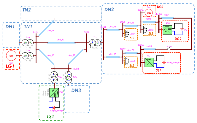
Figure 1: Modern interconnected power systems configuration with active distribution networks.

We use software agents, i.e., pieces of software that are able to speak for, and control, a set of electrical systems. An agent can be associated with a resource, or an entire system including a grid and/or a number of devices. An agent can be implemented in a stand-alone processor, as a process on a control computer, or as an embedded system. Small systems such as appliances, boilers or small photovoltaic roofs do not necessarily need to have a specific agent. Instead, they can be controlled and represented by one single group-aggregating agent that uses a broadcast protocol such as GECN [17, 18]. An agent that controls an entire grid is called “Grid Agent” (GA); other agents are called “Resource Agents” (RAs). Each agent is assigned a role of a leader of one or more other agents that we term the followers of that leader. The roles follow the hierarchy of distribution and transmission networks. For example, in Fig. 1, the grid agent of DN2 is a leader of the resource agents of SS1, DG1, DG2, and SLx. Also, DN2’s Grid Agent is a follower of TN1’s Grid Agent. Resource Agents are always followers, but grid agents can assume both roles. Agents communicate using a simple Advertisement/Request protocol, as follows.

• A follower agent (GA or RA) periodically advertises an abstract view of the internal state of the resource or grid to its leader in the form defined in Section 4.

• A leader agent (GA) has knowledge of the state of its electrical grid and uses the information received from its followers, together with the requested setpoints from its own leader, in order to compute the requested power setpoints of its followers (Section 5); the setpoints are then sent to all the followers.

• On receiving the requested setpoints, the followers set, if possible, their operation according to the requested setpoints and respond with a new advertisement that also serves as a confirmation to the leader that the setpoints were set.

The process is repeated periodically every $T$ time units. In this paper we take $T=100ms$, a value short enough to cope with the fastest possible volatility of distributed resources and large enough to be compatible with the need to estimate the electrical state of the grid. However, this time can be shortened down to the limit of the adopted telecom infrastructure. We also assume that a GA receives measurements from the grid under its responsibility; they are used to estimate the electrical state. The measurement messages are also sent periodically, with a period $\tilde{T}=20ms$. Such a time period is compatible with the data frames of modern monitoring systems equipped, for instance, with phasor measurement units (PMUs). These devices typically provide synchrophasor measurements ranging from 10 to 60 frames-per-second, as required by the IEEE Std. C37.118 [19, 20]. Examples of time latencies and accuracy of real-time state estimation processes fully based on PMU data are discussed in [21, 22]. Typical time latencies of less than $200ms$ can be achieved in order to determine the system state with relevant refresh rates of some tens of milliseconds.

4 Virtual Cost, $PQt$ profile and Belief Function

In this section, we describe the elements of the advertisement messages that are sent by the followers to their leader.

4.1 Virtual Cost and $PQt$ Profile

An agent advertises to its leader a region in the $(P,Q)$ plane (for active and reactive power) that the subsystem, under the control of this agent, can deploy (negative power means consumption). More precisely, the $PQt$ profile advertised by the agent is the set of $(P,Q)$ values that this subsystem is willing to implement in the next iteration. In addition, the agent also advertises a virtual cost function, defined for every $(P,Q)$ in the $PQt$ profile. The virtual cost is interpreted as the cost to this subsystem of applying a requested power setpoint. It is worth observing that this virtual cost does not make reference to a real electricity cost. On the contrary, its role is to quantify the propensity of this subsystem to deploy $(P,Q)$ setpoints within particular zones of the $PQt$ profile. For instance, if the subsystem is a storage system, when the state of charge is close to $100\%$, its agent advertises a negative cost for positive $P$ and positive cost for negative $P$, thus signalling to the grid agent that the storage system would prefer to be discharged. Note that agents do not advertise device specific information such as state of charge; this is an intentional feature of our approach, because keeping the advertised information generic enables aggregation and composition of systems.

4.2 Belief Function

A follower agent also advertises its belief function, which returns the set of all possible (actual) setpoints that this subsystem might implement. Formally, we call $BF$ the belief function of an agent and assume that it receives from its leader GA a request to implement a setpoint $(P,Q)$; then the actual setpoint $(P^{\prime},Q^{\prime})$ that this subsystem does implement lies in the set $BF(P,Q)$ with overwhelming probability.

The belief function accounts for the uncertainty in subsystem operation. In particular, highly controllable subsystems, such as batteries and generators, are expected to have (almost) ideal beliefs, namely $BF(P,Q)=\{(P,Q)\}$. For subsystems such as PV/wind farms, or loads, the belief function will return larger sets, to account for their volatility.

It is important to underline the difference between a $PQt$ profile and a belief function: the former indicates the deployable setpoints that this subsystem is willing to receive, whereas the latter indicates all the possible operating conditions that might result from applying a requested setpoint due to the stochasticity of the process controlled by the resource agent. In particular, the $PQt$ profile represents the domain of definition of both the virtual cost function and the belief function.

Recall that the advertisement messages (with $PQt$ profiles, virtual costs and belief functions) are sent not only by RAs to their GA but also by a GA to its own leader, by means of the composability property described in Section 6.

4.3 Valid Approximations of $PQt$ Profiles and Belief Functions

As our goal is to develop a real-time system that completes its cycle in approximately $100ms$, we often use simplifications. To be valid (i.e., to keep the system in a feasible electrical state), any simplification must satisfy the following property:

Definition 4.1 (Validity Property for $PQt$ profiles and Belief Functions).

$(\mathcal{A}_{i},BF_{i})$ is a valid pair of $PQt$ profile and belief function for a given subsystem $i$ if, whenever this subsystem receives a target setpoint $(P,Q)\in\mathcal{A}_{i}$, the actual power injected by this subsystem lies in the set $BF_{i}(P,Q)$.

As will become clear below, a grid agent can simplify its computation by using approximations of the advertised $PQt$ profiles and belief functions, instead of those sent by the followers, as long as the approximation satisfies the validity property. In particular, if we replace an original $PQt$ profile and belief function by an approximating subset for the $PQt$ profile and approximating supersets for the belief function, then the approximation is valid. We present concrete examples of such simplifications in Sections 5.2.2 and 6.1.

5 The Grid Agent’s Decision Process

In this section, we describe the decision process performed by the Grid Agent (GA), as illustrated in Figure 2. Consider a GA responsible for a grid in which there are $n$ subsystems, each with their own agent $A_{1}...A_{n}$ (recall that some of these subsystems may be entire grids). This GA can also be following a leader grid agent, say GA₀.

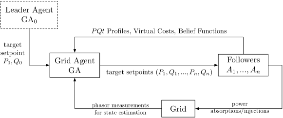
Figure 2: Illustration of the decision process made by GA.

At every time step, this GA receives the $PQt$ profiles, virtual costs and belief functions of followers $A_{1},...,A_{n}$, the target setpoint $(P_{0},Q_{0})$ for the power flow to/from its leader grid (requested by the leader GA₀), and an estimation of the electrical state of the grid. The goal of the GA is then to steer, using frequent updates, the electrical state of its grid by explicitly setting the power setpoints so that (i) the virtual costs of the followers are minimized, (ii) the setpoint $(P_{0},Q_{0})$ is satisfied as much as possible and that (iii) the grid is in a feasible state of operation, as defined in Section 5.1.

To reach its goal, the GA applies its decision process, as described in Section 5.2, and obtains target power setpoints $(P_{1},Q_{1},...,P_{n},Q_{n})$ that are then communicated to the follower agents $A_{1},...,A_{n}$. All subsystems do their best to implement the target setpoints, but subsystem $i$ might end up applying any actual setpoint $(P^{\prime}_{i},Q^{\prime}_{i})\in BF_{i}(P_{i},Q_{i})$ where $BF_{i}$ is the belief function previously advertised by $A_{i}$. The process is then repeated at the next time step.

Observe that in our hierarchy of agents, there can be two possible types of GAs: (i) a GA that is connected to a higher level network with a higher network’s GA being its leader, and (ii) a GA that has no leader and works in an islanded mode (e.g., GA₀ in the above example). We term the former internal GA (representing the internal node in the tree hierarchy) and the latter root GA (representing the root of the tree hierarchy). A root GA naturally relies on a slack resource (such as a storage system or synchronous generator working in the voltage control mode) in order to operate its grid. Thus, in this case, one of the follower agents becomes a slack agent.

In the following subsections, we describe the details of the GA’s decision process, emphasizing the difference between these two types of GAs.

5.1 Feasible State of Operation and Admissible Target Setpoints

In the case of the internal GA, we consider that the grid under the control of the GA is connected to the grid of the leader grid agent, say GA₀, at a point of common coupling (PCC). We assume that GA knows the equivalent Thevenin impedance between the PCC and the slack bus of the overall system. This impedance can be computed using a given methodology such as [23, 24, 25]. Thus, for the computation of the load-flow, we consider as a slack bus the node after this impedance that is included in the admittance matrix of the grid.

In the case of the root GA, the slack bus is naturally the bus where the slack resource is connected.

The electrical state of this grid is given by the set $\{\delta_{k},V_{k}\}$ of the voltage angles and magnitudes at different buses $k$, with $\delta_{0}=0^{\circ}$ and $V_{0}$ is fixed (given) by convention of the slack bus. We assume that the GA has the means to estimate the electrical state of its grid with a sufficient refresh rate compatible with the frequency of power setpoints updates.

We say that an electrical state is feasible if

1. It satisfies static conditions on voltage and currents, of the form

   $$V_{k}\in[V_{k}^{nom}-\beta_{k},V_{k}^{nom}+\beta_{k}],\quad I_{\ell}\leq I_{\ell}^{\max}$$ (1)

   where $V_{k}^{nom}$ is the nominal voltage value of $V_{k}$ (which depends on the voltage rating of the GA’s grid), $I_{\ell}$ is the current magnitude at a line $\ell=(k,k^{\prime})$, and $\beta_{k}$ and $I_{\ell}^{\max}$ are given threshold variables.

2. The power injection at the slack bus is within a specified region $R_{0}$:

   $$(P_{0},Q_{0})\in R_{0}.$$ (2)

Note that, for the sake of clarity, the concept of feasible electrical state defined by (1) and (2) has been intentionally simplified to include only these steady-state feasibility conditions. This concept can be further extended to take into account other conditions that formalize the dynamic stability of a grid such as voltage and angular stability. In this respect, recent literature has discussed the stability aspects of microgrids in the case of constant-power injections/absorptions actuated by modern power electronics (e.g., [26] and [27]). Although this aspect goes beyond the scope of this paper, it is worth observing that for this specific case, as the GA is assumed to know the state of the grid, it also knows the admittance matrix of the system. As a consequence, it can formally compute the frequency-domain input impedances in the correspondence of each node where the resources are connected. Therefore, the GA can potentially use this information to augment the computation of the feasible electrical state of the grid and, thus, include further stability requirements.

We are interested in radial distribution networks, in which it is known that the load-flow problem has a unique solution if voltage magnitudes are close to nominal values [28, 29]. We consider a grid operating in this regime. In particular, we assume that the voltage magnitude bounds $\beta_{k}$ are small enough to guarantee the uniqueness of a solution to the load flow equation and that it contains a margin compatible with the accuracy of state estimation. This implies that the electrical state of the grid and the power flow at the PCC are uniquely determined by the injections/absorptions at all subsystems $(P_{1},Q_{1},...,P_{n},Q_{n})$ and the voltage $(\delta_{0},V_{0})$ at the slack bus.

We aim at controlling the power setpoints at all subsystems, which therefore allows to control the electrical state of the grid. However, the actual power setpoints implemented by subsystems can differ from targets, and this is captured by the belief functions. This suggests the following definition.

Definition 5.1 (Admissible Target Setpoints).

We say that a collection of target setpoints $(P_{1},Q_{1},...,P_{n},Q_{n})$ is admissible if for any actual implementation that is compatible with the belief function, the resulting electrical state is feasible. We denote the admissible set by $\mathcal{U}$.

5.2 Formulation of the Objective Function and Overview of The Decision Process

The goal of the grid agent GA is to compute the collection

$$u=(P_{1},Q_{1},...,P_{n},Q_{n})$$ (3)

of target setpoints that it will send to its followers. In order to do so, the virtual costs of the followers are aggregated by means of the weighted total cost

$$C(u)\triangleq\sum_{i=1}^{n}w_{i}C_{i}(P_{i},Q_{i}),$$ (4)

where $C_{i}$ is the virtual cost function of follower $i$, and the weights $\{w_{i}\}$ express the preference of GA of one follower over another.

In particular, GA would put a higher weight on the cost function of a device that provides more service to the grid and is more controllable. For example, more weight can be put on storage systems, whereas less weight on loads and semi-controllable generators (such as PV or wind farms). The optimal computation of the weights is out of the scope of this paper. We just mention that, in general, some adaptive learning procedures can be applied to adjust the weights based on the observed history of the followers. In this paper, we assume that the weights are pre-computed based on the prior knowledge on the followers and that they are fixed during the system’s operation.

Further, we add a penalty term that represents the constraints on the power at the PCC/slack bus. Here and below, we use a superscript $(I)$ to denote the variables related to the internal GA, and $(R)$ to denote these of the root GA. In the case of the internal GA, it needs to accommodate the request $(P_{0},Q_{0})$ sent by its leader agent GA₀; this is captured by adding to the virtual cost a penalty term

$$J_{0}^{(I)}(P_{0},Q_{0};P_{0}(u),Q_{0}(u))$$

where $J_{0}(\cdot)$ is some measure of the distance between $(P_{0},Q_{0})$ and $(P_{0}(u),Q_{0}(u))$. Here, $(P_{0}(u),Q_{0}(u))$ is the resulting power flow through the PCC when the collection of power flows at other systems is given by $u$. In this paper, we use the function $J_{0}$ defined by

$$J_{0}^{(I)}((P_{0},Q_{0}),(P^{\prime}_{0},Q^{\prime}_{0}))=w_{0}((P_{0}-P^{\prime}_{0})^{2}+(Q_{0}-Q^{\prime}_{0})^{2})$$

for $w_{0}>0$. On the other hand, as the root GA works in an islanded mode, there is no request for the power at the connection point. Instead, we use the advertised cost of the slack agent as a cost for power at the slack bus, namely

$$J_{0}^{(R)}((P_{0},Q_{0}),(P^{\prime}_{0},Q^{\prime}_{0}))=w_{0}C_{0}(P^{\prime}_{0},Q^{\prime}_{0}),$$

where $C_{0}$ is the cost advertised by the slack agent.

Finally, a penalty term $J(u)$ is added to capture the distance of the electrical state to the boundary of the feasible region. This function is defined in terms of both threshold variables $\beta_{k}$ and $I_{\ell}^{\max}$. In this paper, we consider that the first is constant (e.g., 10% of the nominal voltage), whereas the second might change dynamically. In particular, we allow a line to transfer current over its ampacity limit by considering the specific energy of its conductor, normally available from the manufacturer. With this, $I_{\ell}^{max}$ is computed as the current that makes the Joule Integral $\int I_{\ell}(t)^{2}dt$ reach the specific energy characteristic.

In this paper we use the function $J$ defined by

$$J(u) \triangleq \sum_{k}\frac{(V_{k}(u)-V_{k}^{nom})^{2}}{\beta_{k}^{2}-(V_{k}(u)-V_{k}^{nom})^{2}}+\sum_{\ell}\frac{I_{\ell}(u)^{2}}{(I_{\ell}^{max})^{2}-I_{\ell}(u)^{2}}$$

if $$\{V_{k}(u),I_{\ell}(u)\}$$ satisfy (1)

$$= \infty\mbox{ otherwise.}$$

In the above $V_{k}(u)$, $I_{\ell}(u)$ are the voltage and current magnitudes that result from the load-flow solution when the collection of power injections/absorptions is given by $u$.

Ideally, GA would like to find a collection of target setpoints $u$ that (i) is admissible (as per Definition 5.1) and (ii) minimizes

$$C(u)+J_{0}(P_{0},Q_{0};P_{0}(u),Q_{0}(u))+J(u)$$ (6)

over all admissible $u$.

However this is not easily computable. Instead, we propose to steer the power injections in the direction of the optimum of (6), using a gradient descent approximation. More precisely, the decision process at the grid agent computes

$$\begin{array}[]{l}u=\mathscr{P}_{\mathcal{U}}\Big{\{}\hat{x}-\alpha\nabla_{u}\big{[}C(u)+J_{0}(P_{0},Q_{0};P_{0}(u),Q_{0}(u))+J(u)\big{]}\Big{|}_{u=\hat{x}}\Big{\}},\end{array}$$ (7)

where $\mathscr{P}_{\mathcal{U}}$ is the Euclidean “projection” to the admissible set $\mathcal{U}$, $\hat{x}=(\hat{P}_{1},\hat{Q}_{1},...,\hat{P}_{n},\hat{Q}_{n})$ is the last estimated power setpoint (obtained from the GA’s state estimation process), and $\alpha$ is a step size parameter.

Note that the algorithm defined in (7) requires two major computations: (i) that of the gradient of the objective function, and (ii) the projection to $\mathcal{U}$. We next describe the methods that are used in this paper in order to perform these computations in real time.

5.2.1 Gradient of the Objective Function

By using the definition of $J$ in 5.2, it can be easily verified that

$$\nabla_{x}J(x)=\sum_{k}\frac{2\beta^{2}(V_{k}(x)-V^{nom})}{(\beta^{2}-(V_{k}(x)-V^{nom})^{2})^{2}}\nabla_{x}V_{k}(x)\\ +\sum_{\ell}\frac{2(I_{\ell}^{max})^{2}((I_{\ell}^{max})^{2}-I_{\ell}(u)^{2})}{\left((I_{\ell}^{max})^{2}-I_{\ell}(u)^{2}\right)^{2}}\nabla_{x}I_{\ell}(x).$$ (8)

This requires the knowledge of $V_{k}(x)$ and $I_{\ell}(x)$ and, in particular, its dependence on the setpoint $x$. The exact dependence is complicated, as it follows from the solution of the power flow equations. We use, instead, a linear approximation of this dependence. In particular, given the current state $\hat{V}=\{\hat{V}_{k}\}$ and $\hat{I}=\{\hat{I}_{\ell}\}$ (obtained from the state estimation procedure), we let $\widetilde{V}(x)=\hat{V}+K_{V}(x-\hat{x}),\text{ and }\widetilde{I}(x)=\hat{I}+K_{I}(x-\hat{x}),$ where $K_{V}$ and $K_{I}$ are the voltage and current sensitivity coefficients computed using methods as in [30, 31]. By using this approximation, we have that $\nabla_{x}\widetilde{V}_{k}(x)=(K_{V})_{k}$ and $\nabla_{x}\widetilde{I}_{k}(x)=(K_{I})_{k}$. Moreover, as the gradient $\nabla_{x}J(x)$ is computed at $x=\hat{x}$, we have that $\widetilde{V}(x)=\hat{V}$ and $\widetilde{I}(x)=\hat{I}$. Therefore, Equation (8) and the approximated values above provide us with an approximation of the gradient of the objective function.

A similar approach is taken in order to compute the gradient of $J_{0}(u_{0},X_{0}(x))$, where $X_{0}(x)=(P_{0}(x),Q_{0}(x))$: the exact dependence of $X_{0}(x)$ is replaced by an approximated linear one, and the corresponding gradient is computed. Finally, the gradient of the cost function $C(x)$ is computed either by using the analytical form of the cost function advertised to GA, or by numerical approximation.

5.2.2 Computation of the Beliefs and Projection to the Admissible Set

We next give explicit expressions for the admissible sets used in both types of grid agents. For clarity, we now need to introduce some more notations. We denote with $\mathcal{A}$ the joint $PQt$ profile, i.e. set of all collections of setpoints that are in the advertized $PQt$ profiles. Namely, $\mathcal{A}\triangleq\Pi_{i=1}^{n}\mathcal{A}_{i}$, where $\mathcal{A}_{i}$ is the $PQt$ profile advertised by follower $i$ and $\Pi_{i=1}^{n}$ stands for the Cartesian product of sets. Similarly, we denote with $BF$ the joint belief function, defined for all $u=(P_{1},P_{2},...,P_{n},Q_{n})\in\mathcal{A}$ by $BF(u)\triangleq\Pi_{i=1}^{n}BF_{i}(P_{i},Q_{i})$. Note that $\mathcal{A}$ represents the domain of definition of the two functions $C(u)$ and $BF(u)$.

Since the internal GA works in grid-connected mode, we assume that there is no explicit constraint on the power flow at the PCC (namely, constraint (2) is inactive). Hence, the admissible set can be written as

$$\mathcal{U}^{(I)}\triangleq\left\{u\in\mathcal{A}^{(I)}:\forall x\in BF^{(I)}(u),\,J^{(I)}(x)<\infty\right\},$$ (9)

where $x=(P^{\prime}_{1},Q^{\prime}_{1},...,P^{\prime}_{n},Q^{\prime}_{n})$ is any actual implementation of the setpoints. Observe that, in this case, the feasibility condition (1) is equivalent to $J^{(I)}(x)<\infty$ (see (5.2)). In the admissible set of the root GA, on the contrary, the feasibility condition (2) is active, as it takes into account the capability limits of the slack resource. In particular,

$$\mathcal{U}^{(R)}\triangleq\left\{u\in\mathcal{A}^{(R)}:\forall x\in BF^{(R)}(u),\,J^{(R)}(x)<\infty\text{ and }X^{(R)}_{0}(x)\in\mathcal{A}^{(R)}_{0}\right\},$$ (10)

where $\mathcal{A}^{(R)}_{0}$ is the $PQt$ profile of the slack resource, and $X^{(R)}_{0}(x)$ is the power injected/absorbed by it when the power setpoint of the other followers is $x$.

We next relax the exact computation of the projection to the set of admissible target setpoints $\mathcal{U}$, which is required in algorithm (7). Note that belief functions are used to ensure a feasible operation of the grid, hence we need to guarantee that the relaxation maintains the feasibility property.

For brevity, we focus in the rest of this subsection on the internal GA; similar computations are preformed in the root GA. First, consider the subproblem of testing whether a given control $u$ is in $\mathcal{U}$. We refer to this process as the admissibility test. As follows from (9), in order to carry out this test, we should solve $\max_{x\in BF(u)}J(x)$ and verify whether the result is finite.

The above optimization is hard in general, hence we propose to relax it as follows. First, observe that using Definition 4.1, we can replace the exact belief functions with supersets. We thus assume that the grid agent has access to functions $\overline{BF}_{i}(P_{i},Q_{i})$ with the following two properties: (i) $BF_{i}(P_{i},Q_{i})\subseteq\overline{BF}_{i}(P_{i},Q_{i})$, and (ii) $\overline{BF}_{i}(P_{i},Q_{i})$is a rectangle in ². We note that the rectangular super beliefs can be either sent directly by the follower agents, or computed by the grid agent from the advertised exact beliefs.

In addition, we use the following property of the load-flow solution that holds true in the networks considered in this paper. It was shown in [29] that the solution is monotonic in radial distribution networks, whenever the shunt elements of the lines are neglected. Specifically, every voltage magnitude can either increase or decrease monotonically as a function a single power injection (while the other injections are kept fixed). Similarly, the extreme values of the current magnitudes are obtained at the extreme values of a power injection. By using the definition of $J$ in (5.2), it follows that only a small finite number of simple computations is required in order to perform the admissibility test of a control $u$. In particular, for each vertex $v$ of $\overline{BF}(u)$, we should test whether (i) there exists a solution to the load-flow equations, and (ii) $J(v)<\infty$.

Given this simplified admissibility test, we can devise an efficient method for projection to $\mathcal{U}$. As the projection is needed only in a local vicinity of the current setpoint $\hat{x}$, it can be efficiently computed by doing a search of the closest point in $\mathcal{U}$, and using a relatively small number of the (simplified) admissibility tests. We present the details of the related algorithms in A.

6 Composition of Subsystems

A key aspect of our framework is composability: subsystems can be aggregated and viewed by others as a single entity that exhibits the same properties of a single subsystem (i.e., $PQt$ profile, virtual cost, and belief function). This is essential for the application of the method to systems of any size and complexity.

To illustrate the idea, we consider a radial power network shown schematically in Fig. 3 and two settings of agents depicted in Fig. 4. In the flat setting of Fig. 4 (a), there is a single grid agent (which is a root GA) that is responsible for the whole grid (Grid₀, Grid₁, and Grid₂) and is a leader of $N_{1}+N_{2}$ agents $A_{11},...,A_{1,N_{1}},A_{21},...,A_{2N_{2}}$. In the hierarchical setting of Fig. 4 (b), there are three grid agents GA₀, GA₁, and GA₂, each responsible for Grid₀, Grid₁, and Grid₂, respectively. Consequently, in the hierarchical setting, GA₁ is an internal GA that is the leader of $N_{1}$ agents $A_{11},...,A_{1N_{1}}$, GA₂ is an internal GA that is the leader of $N_{2}$ agents $A_{21},...,A_{2N_{2}}$, and GA₀ is a root GA that is the leader of GA₁ and GA₂.

In this case, GA₁ and GA₂ represent their internal state to GA₀ by advertising aggregated $PQt$ profiles, virtual costs, and belief functions. To define these elements, consider the follower grid agent GA₁, aggregating and sending advertisements to its leader grid agent GA₀. First, GA₁ computes the aggregated PQt profile as the set of all possible power flows $(P^{1}_{0},Q^{1}_{0})$ at the PCC of Grid₁ and Grid₀, given that the powers injected by the followers of GA₁ belong to their respective $PQt$ profiles, advertised to GA₁; this is computed by solving the load-flow for Grid₁. Second, GA₁ computes the value of the aggregated virtual cost function for every $(P^{1}_{0},Q^{1}_{0})$ that is in the aggregated $PQt$ profile as follows: GA₁ applies its decision process in order to obtain a collection of power setpoints for its set of followers and returns the corresponding value of the objective function (6). Last, the value of the aggregated belief function at $(P^{1}_{0},Q^{1}_{0})$ is the set equal to the union of all possible actual power flows at the PCC of Grid₁ and Grid₀ over all possible actual power injections at the followers, given by the belief functions advertised to GA₁.

In theory, such an aggregation is transparent, i.e., the operation of the grid is the same in both the flat and the hierarchical settings. More precisely, assume that

1. The two systems in Fig. 4 (a) and (b) are synchronized in communication exchange;

2. There is no delay in the transmission of information over the channels;

3. Both GA₁ and GA₂ know the exact equivalent Thevenin impedance between their PCC and the slack bus of the overall system;

4. All the grid agents implement the optimal control defined by the optimization (6), with the penalty function $J_{0}$ given by

   $$J_{0}(P_{0},Q_{0};u_{0})=\begin{cases}0,&\text{ if }(P_{0},Q_{0})=u_{0},\\ \infty,&\text{ otherwise.}\end{cases}$$

   (Namely, we have a strict constraint $(P_{0},Q_{0})=u_{0}$ at the PCC.)

Figure 3: Schematic representation of a radial distribution network.

Figure 4: (a) A flat architecture, with one centralized grid agent. (b) A hierarchical architecture, with three grid agents.

Proposition 6.1.

In the ideal case defined above, the target power setpoints computed at one step of the decision process are the same in both settings of Fig. 4 (a) and (b).

The proof of this proposition can be found in the Appendix.

In Part II of this paper, we propose practical methods for computing the aggregated elements described above and we show their performance.

6.1 Aggregated $PQt$ Profile and Belief Function

In order to aggregate in practice the $PQt$ profiles and belief functions of an internal GA, we use the validity property formulated in Definition 4.1.

To this end, we first write the load-flow constraints more explicitly, in terms of the power injections in the grid and the powers at the slack bus:

$$P_{0}=\sum_{i=1}^{N}P_{i}-L_{P}(\{P_{i},Q_{i}\}),\quad Q_{0}=\sum_{i=1}^{N}Q_{i}-L_{Q}(\{P_{i},Q_{i}\}),$$ (11)

where $L_{P}(\{P_{i},Q_{i}\})\geq 0$ and $L_{Q}(\{P_{i},Q_{i}\})$ is the active and reactive total power loss. Alternatively, (11) can be written as

$$X_{0}(u)=\sum_{i}u_{i}-L(u),\quad L(u)\triangleq(L_{P}(\{P_{i},Q_{i}\}),L_{Q}(\{P_{i},Q_{i}\})),$$

and the exact aggregated $PQt$ profile reads

$$\widetilde{\mathcal{A}}_{0}=\bigcup_{u\in\mathcal{U}}\left\{u_{0}=\sum_{i}u_{i}-L(u)\right\}.$$ (12)

Our method for approximation is based on (i) omitting the loss term when computing the aggregated $PQt$ profile, and (ii) accounting for the resulting error in the aggregated belief function. Next, we describe these two procedures in detail.

Computing the aggregated $PQt$ profile:

• Given the current setpoint $\hat{x}$ (again, assumed as known via a state-estimation process), randomly and uniformly generate $M$ setpoints $u^{k}\in\mathcal{A}$, $k=1,...,M$ with the following two properties:

  • Locality: $\left\|u^{k}-\hat{x}\right\|\leq\alpha G_{\max}$, where $\alpha$ is the step size of the gradient descent algorithm (7) and $G_{\max}$ is an upper bound for the gradient.

  • Admissibility:

    $$\forall x\in\operatorname{conv}\left\{BF(u^{k})\right\},\quad J(x)<\infty,$$ (13)

    where $\operatorname{conv}\left\{BF(u^{k})\right\}$ is the convex hull of the sets defined by the belief functions $BF(u^{k}),k=1,...,M$. Observe that (13) is a stronger requirement than just $u^{k}\in\mathcal{U},k=1,...,M$. This step can be performed efficiently by using local methods for projection described in A. In particular, similarly to the methods described in Section 5.2.2, $\operatorname{conv}\left\{BF(u^{k})\right\}$ can be overapproximated by a rectangular set, and the feasibility property is then trivially tested only on the vertices of the rectangle.

• Compute the corresponding ideal powers at the slack bus $u_{0}^{k}=\sum_{i=1}^{N}u_{i}^{k}$, and advertize the following approximation for the aggregated $PQt$ profile:

  $$\widetilde{\mathcal{A}}^{*}_{0}=\operatorname{conv}(\{u_{0}^{k}\}_{k=1}^{M}),$$ (14)

  namely the convex hull of $\{u_{0}^{k}\}_{k=1}^{M}$.

The belief functions can be aggregated by solving the following four optimal power flow problems (OPFs) for a each $u_{0}\in\widetilde{\mathcal{A}}_{0}^{*}$:

$$\begin{array}[]{l}\max/\min P_{0}\\ \text{s.t.}\begin{cases}x\in BF(F(u_{0})),&\\ (P_{0},Q_{0})=X_{0}(x),&\\ \end{cases}\end{array}\text{ }\begin{array}[]{l}\max/\min Q_{0}\\ \text{s.t.}\begin{cases}x\in BF(F(u_{0})),&\\ (P_{0},Q_{0})=X_{0}(x),&\\ \end{cases}\end{array}$$ (15)

where $u=F(u_{0})$ represents the algorithm of (7). This will yield a rectangular belief function that represents a superset of the true aggregated belief. In this paper, due to timing constraints, we avoid solving these exact OPFs; instead we use (11) and bounds on the losses. As a preliminary step, these bounds are estimated offline:

$$\overline{L}_{P}=\max L_{P}(\{P_{i},Q_{i}\}),\quad\underline{L}_{P}=\min L_{P}(\{P_{i},Q_{i}\}),$$

$$\overline{L}_{Q}=\max L_{Q}(\{P_{i},Q_{i}\}),\quad\underline{L}_{Q}=\min L_{Q}(\{P_{i},Q_{i}\}),$$

where the optimization is done over all possible setpoints.

Computing the aggregated belief function:

• Generate a uniform partition $\mathcal{P}_{0}$ over $\widetilde{\mathcal{A}}^{*}_{0}$. A given requested setpoint $u_{0}\in\widetilde{\mathcal{A}}^{*}_{0}$ is mapped into a representative request $u_{0}^{\mathcal{P}}\in\mathcal{P}_{0}$ (e.g., the closest point to $u_{0}$ in $\mathcal{P}_{0}$).

• For each $u_{0}^{\mathcal{P}}\in\mathcal{P}_{0}$, compute

  1. The corresponding setpoints for the followers $u=\{u_{i}\}=F\left(u_{0}^{\mathcal{P}}\right)$.

  2. The bounds for the power at the connection point, using the bounds on the losses:

     $$P_{0}^{\max}(u_{0}^{\mathcal{P}})=\max_{(P_{i},Q_{i})\in BF_{i}(u_{i})}\sum_{i}P_{i}-\underline{L}_{P},\quad P_{0}^{\min}(u_{0}^{\mathcal{P}})=\min_{(P_{i},Q_{i})\in BF_{i}(u_{i})}\sum_{i}P_{i}-\overline{L}_{P},$$ (16)

     and similarly for $Q_{0}^{\max}(u_{0}^{\mathcal{P}})$ and $Q_{0}^{\min}(u_{0}^{\mathcal{P}})$. Observe that if $BF_{i}$ are rectangular, (16) is just the summation of the corresponding individual upper/lower bounds.

• Advertise the resulting belief function over $\mathcal{P}_{0}$ with the interpretation that for each $u_{0}\in\widetilde{\mathcal{A}}^{*}_{0}$,

  $$\widetilde{BF}^{*}_{0}(u_{0})=\left[P_{0}^{\min}(u_{0}^{\mathcal{P}}),P_{0}^{\max}(u_{0}^{\mathcal{P}})\right]\times\left[Q_{0}^{\min}(u_{0}^{\mathcal{P}}),Q_{0}^{\max}(u_{0}^{\mathcal{P}})\right],$$ (17)

  where $u_{0}^{\mathcal{P}}$ is the representative element for $u_{0}$ in $\mathcal{P}_{0}$.

It follows from this construction that for any request $u_{0}\in\widetilde{\mathcal{A}}^{*}_{0}$, the actual power at the connection point $x_{0}$ satisfies that $x_{0}\in\widetilde{BF}^{*}_{0}(u_{0})$. In other words, the pair $(\widetilde{\mathcal{A}}^{*}_{0},\widetilde{BF}^{*}_{0})$ is a valid pair of a $PQt$ profile and a belief function as per Definition 4.1.

We note that the previous statement does not pose any requirements on the accuracy of the aggregated $PQt$ profile $\widetilde{\mathcal{A}}^{*}_{0}$. In fact, it is valid for any $\widetilde{\mathcal{A}}^{*}_{0}$ provided that the belief function is constructed as above. The next result shows that when the losses are small and the belief functions satisfy a certain concavity property, the proposed construction for $\widetilde{\mathcal{A}}^{*}_{0}$ provides us with a good approximation of the true aggregated $PQt$ profile. The proof can be found in C.

Theorem 6.1.

Suppose that $BF(u)$ is a concave set-valued function, namely for all $u_{1},u_{2}\in\mathcal{A}$ and $\alpha\in[0,1]$

$$BF(\alpha u_{1}+(1-\alpha)u_{2})\subseteq\alpha BF(u_{1})+(1-\alpha)BF(u_{2})$$

(where the second plus sign stands for the Minkowski sum). Then $\widetilde{\mathcal{A}}^{*}_{0}$ is a convex $\delta$-approximation of the exact $PQt$ profile $\widetilde{\mathcal{A}}_{0}$ (12), with $\delta\triangleq\max_{x}\left\|L(x)\right\|$. Namely, for any $x_{0}^{\prime}\in\widetilde{\mathcal{A}}^{*}_{0}$ there exists $x_{0}\in\widetilde{\mathcal{A}}_{0}$ such that $\left\|x_{0}-x_{0}^{\prime}\right\|\leq\delta$.

It can be verified that the concavity requirement of $BF(u)$ holds for the resources considered in the case study in Part II of this paper.

Remark. As follows from Theorem 6.1, the proposed construction for the approximate aggregated $PQt$ profile is a good approximation of the exact aggregated $PQt$ profile whenever the bound on the losses $\delta\triangleq\max_{x}\left\|L(x)\right\|$ is small. Hence, this approximation can be successfully used in the LV networks, such as the microgrid case in our paper. However, it is possible to compute an approximation to the aggregated $PQt$ profile also in other cases where the losses are not negligible (such as the MV network in the case study). For example, instead of omitting the losses when computing (14), we can solve the exact load-flow problem for each $u^{k}$ in order to obtain the exact power at the PCC $u_{0}^{k}$. Furthermore, as mentioned above, the computation of the aggregated belief function can be made more accurate as well, by solving the OPFs (15). This will certainly provide us with better approximations in the case of networks where losses are high. However, the resulting procedures will be more demanding computationally. In particular, a special procedure should be devised in order to choose a small set of representative candidate setpoints $u^{k}$, hence reducing the overall computational complexity. This is out of the scope of this paper.

6.2 Aggregated Cost Function

As was already mentioned, for computing the aggregated virtual cost function at a given requested setpoint at the PCC $u_{0}=(P_{0},Q_{0})$, the internal GA applies its gradient descent algorithm (7) in order to obtain a collection of power setpoints $u$ for its set of followers, and it returns the corresponding value of the objective function (6). In this paper, in order to advertize the virtual cost for every $u_{0}\in\widetilde{\mathcal{A}}^{*}_{0}$, we compute it on a sparse partition of the aggregated $PQt$ profile $\widetilde{\mathcal{A}}^{*}_{0}$ and advertize a linear interpolation thereof.

7 Conclusion

We have described the elements of a method that uses explicit power setpoints in order to control electrical grids in a scalable and reliable way. The proposed approach enables the behaviour of a complex electrical system to emerge as a property of a combination of agents, irrespective of the stochastic or deterministic nature of the energy resources. In this respect, a first feature of this Part I is to guarantee that any system that implements the proposed framework must be correctly controllable by construction. The correctness of the control is such that it guarantees not only a feasible operation point but, also, some form of optimality. This is achieved by combining the cost of the grid and the virtual costs of the resources. The proposed framework has been designed to manage, by leveraging on the abstraction of the devices state, systems characterized by high volatility of energy resources. This property guarantees the inherent minimization of the required reserve usually needed in traditional control schemes for power systems.

A second feature of the proposed framework is composability. The same abstraction and protocol is used uniformly, regardless of the specifics of the resources or sets of resources and of system size. The rules for the abstraction of devices and subsystems have been provided, together with the proof of the main aggregation property. This allows an entire network and its resources to be viewed and handled as a single resource: this is a key characteristic, as it enables the method to be scaled to systems of any size.

In Part II, we use a practical case study to demonstrate a detailed implementation of the method and we evaluate its performance benefits.

Appendix A Algorithms

Algorithm 1: Admissibility Test

• Input: Control $u=(u_{j})$ to be tested.

• Parameters: Belief functions of the resources, given in terms of $\mathcal{B}_{j}(u_{j})$ – finite sets of representative “worst-case” setpoints that $u$ can give rise to (e.g., vertices of a rectangular belief).

• Do: Obtain worst-case setpoints of a resource $j$ by using the belief function, $B_{j}=\mathcal{B}_{j}(u_{j}),$ and test all possible combinations of the setpoints in $B_{j}$. That is, for each $x_{j}\in B_{j}$, compute $d\left(x,\mathcal{Y}\right)$, where $d(y,\mathcal{Y})$ is a certain “distance” of $x$ from the set $\mathcal{Y}\triangleq\{x:\,J(x)<\infty\}$. This distance can be computed using the definition of $J$ in Part I, Equation (5).

• Output: Maximum violation $\Delta_{\max}=\max_{x:\,x_{j}\in B_{j}}d\left(x,\mathcal{Y}\right)$.

Algorithm 2: Projection onto $\mathcal{U}$

• Input: Control $u=(u_{j})$ to be projected.

• Parameters: Search step $\Delta u$, number of search directions $n$.

• Initialization: The min-max violation $\Delta_{\min\max}=C>0$.

• While $\Delta_{\min\max}>0$:

  • Generate $n$ test point $\{x_{m},m=1,...,n\}$ uniformly spread on a sphere with radius $\Delta u$ around $u$, so that $\left\|x_{m}-u\right\|=\Delta u$.

  • For $m=1,...,n$:

    • Project $x_{m}$ to $\mathcal{A}$ (using, e.g., the alternating projections method [32]): $x_{m}:=\mathscr{P}_{\mathcal{A}}\left\{x_{m}\right\}.$

    • Use Algorithm 1 to test admissibility of $x_{m}$, save the output to $\Delta_{m,\max}$.

  • Compute the direction of the minimum violation: $m^{*}\in\operatornamewithlimits{argmin}_{m=1,...,n}\Delta_{m,\max},$ and the corresponding violation: $\Delta_{\min\max}=\min_{m=1,...,n}\Delta_{m,\max}.$

  • Update $u:=x_{m^{*}}$.

• Output: The projected control $u$.

Appendix B Proof of Proposition 6.1

Consider first the flat setting of Figure 4 (a). Let $\textbf{u}=(\textbf{u}_{1},\textbf{u}_{2})$ denote the collection of setpoints in the overall grid of Figure 3. The goal of GA is to minimize (subject to constraints) $C(\textbf{u})+J(\textbf{u})$, where, as before, $C(\textbf{u})=\sum_{j=1}^{N_{1}}w_{1j}C_{1j}(u_{1j})+\sum_{j=1}^{N_{2}}w_{2j}C_{2j}(u_{2j})$ is the total cost advertised by the followers and $J(\textbf{u})$ is the internal objective function of GA, which captures the distance of the electrical state to the boundary of the feasible region, as in (5.2). Naturally, the virtual cost is separable, namely $C(\textbf{u})=C_{1}(\textbf{u}_{1})+C_{2}(\textbf{u}_{2}),$ where $C_{i}(\textbf{u}_{i})$ is the advertised cost of the followers in grid $i=1,2$. The penalty function $J(\textbf{u})$ is also separable in the sense: $J(\textbf{u})=J_{1}(\textbf{u}_{1})+J_{2}(\textbf{u}_{2})+J_{0}(X_{1}(\textbf{u}_{1}),X_{2}(\textbf{u}_{2})),$ where $J_{i}$ is the penalty function in grid $i=0,1,2$, and $X_{1}(\textbf{u}_{1})$ (respectively, $X_{2}(\textbf{u}_{2})$) is the power at the PCC between grid $1$ (respectively, $2$) and grid $0$ at the given setpoint $\textbf{u}_{1}$ (respectively, $\textbf{u}_{2}$), when the perfect knowledge of the corresponding equivalent Thevenin impedance is assumed.

Now, without constraining u to the admissible setpoints dictated by the belief functions, the optimization problem of GA in the flat setting is

$$\min_{\textbf{u}}\left(C(\textbf{u})+J(\textbf{u})\right)$$

$$=\min_{u_{1},u_{2}}\left\{\min_{\textbf{u}_{i},X_{i}(\textbf{u}_{i})=u_{i},i=1,2}\left[C_{1}(\textbf{u}_{1})+C_{2}(\textbf{u}_{2})+J_{1}(\textbf{u}_{1})+J_{2}(\textbf{u}_{2})+J_{0}(X_{1}(\textbf{u}_{1}),X_{2}(\textbf{u}_{2}))\right]\right\}$$

$$=\min_{u_{1},u_{2}}\bigg{\{}J_{0}(u_{1},u_{2})+\min_{\textbf{u}_{1},X_{1}(\textbf{u}_{1})=u_{1}}\left[C_{1}(\textbf{u}_{1})+J_{1}(\textbf{u}_{1})\right]+\min_{\textbf{u}_{2},X_{2}(\textbf{u}_{2})=u_{2}}\left[C_{2}(\textbf{u}_{2})+J_{2}(\textbf{u}_{2})\right]\bigg{\}}.$$

Observe that the outer optimization problem is the problem solved by the grid agent GA₀ in the hierarchical setting of Figure 4 (b), not considering the admissibility constraints.

We next take the constraints into account. Let $\mathcal{U}$ denote the set of admissible setpoints of grid agent GA in the flat setting of Figure 4 (a). Similarly, let $\mathcal{U}_{1}$ and $\mathcal{U}_{2}$ denote the set of admissible setpoints of grid agents GA₁ and GA₂ in the hierarchical setting of Figure 4 (b); these sets are computed using the perfect knowledge of the corresponding equivalent Thevenin impedances. Finally, let $\mathcal{U}_{0}$ denote the set of admissible setpoints of grid agent GA₀; this set is computed using the aggregated belief functions advertised by GA₁ and GA₂ (as explained in Section 6). Now, it is easily seen that, under the assumed ideal conditions, the target setpoint u is in $\mathcal{U}$ if and only if $\textbf{u}_{1}\in\mathcal{U}_{1}$, $\textbf{u}_{2}\in\mathcal{U}_{2}$, and $\left(X_{1}(\textbf{u}_{1}),X_{2}(\textbf{u}_{2})\right)\in\mathcal{U}_{0}$, completing the proof of the Proposition.

Appendix C Proof of Theorem 6.1

First, note that, by the concavity of $BF(u)$, we have that

$$\operatorname{conv}\left\{BF(u^{k})\right\}\supseteq BF\left(\operatorname{conv}\left\{u^{k}\right\}\right).$$

Thus, by (13), any $u\in\mathcal{C}\triangleq\operatorname{conv}(\{u^{k}\}_{k=1}^{M})$ satisfies

$$\forall x\in BF(u),\quad J(x)<\infty,$$

implying that $\mathcal{C}\subseteq\mathcal{U}$.

Let

$$\widetilde{\mathcal{A}}^{\prime}_{0}=\bigcup_{u\in\mathcal{U}}\left\{u_{0}=\sum_{i}u_{i}\right\}.$$

Now, $\widetilde{\mathcal{A}}^{\prime}_{0}$ is a $\delta$-approximation of $\widetilde{\mathcal{A}}_{0}$ where $\delta=\max_{x\in\mathcal{X}}\left\|L(x)\right\|$. We thus show below that $\widetilde{\mathcal{A}}^{*}_{0}\subseteq\widetilde{\mathcal{A}}^{\prime}_{0}$, implying that $\widetilde{\mathcal{A}}^{*}_{0}$ is a $\delta$-approximation of $\widetilde{\mathcal{A}}_{0}$ as well. Indeed, let $u_{0}\in\widetilde{\mathcal{A}}^{*}_{0}$. Hence, there exist $\{\gamma_{k}\}_{k=1}^{M}$, $\gamma_{k}\geq 0$, $\sum_{k}\gamma_{k}=1$, so that

$$u_{0}=\sum_{k=1}^{M}\gamma_{k}u_{0}^{k}=\sum_{k=1}^{M}\gamma_{k}\sum_{i}u_{i}^{k}=\sum_{i}\sum_{k=1}^{M}\gamma_{k}u_{i}^{k}=\sum_{i}u^{*}_{i},$$

with

$$u^{*}\triangleq\sum_{k}\gamma_{k}u^{k}\in\mathcal{C}\subseteq\mathcal{U}$$

Therefore, $u_{0}\in\widetilde{\mathcal{A}}^{\prime}_{0}$.

References

- [1] Observ’ER, 14th inventory of worldwide electricity production from renewable energy sources (2012).
- [2] D. MacKay, Sustainable Energy-Without the Hot Air, UIT Cambridge, 2008.
- [3] K. Papadogiannis, N. Hatziargyriou, Optimal allocation of primary reserve services in energy markets, IEEE Transactions on Power Systems 19 (1) (2004) 652–659.
- [4] European Network of Transmission System Operator for Electricity (ENTSO-E), UCTE Operation Handbook, Tech. Rep. v. 2.5 (2004).
- [5] European Network of Transmission System Operator for Electricity (ENTSO-E), Draft network code on demand connection, Tech. rep. (December 5 2012).
- [6] N. Troy, D. Flynn, M. OMalley, Multi-mode operation of combined-cycle gas turbines with increasing wind penetration, IEEE Transactions on Power Systems 27 (1) (2012) 484–492.
- [7] B. Davie, A. Charny, J. C. R. Bennet, K. Benson, J.-Y. Le Boudec, W. Courtney, D. Stiliadis, An expedited forwarding PHB (per-hop behavior), Tech. rep., Internet RFC 3246 (2002).
- [8] T. Wu, Q. Yang, Z. Bao, W. Yan, Coordinated energy dispatching in microgrid with wind power generation and plug-in electric vehicles, IEEE Transactions on Smart Grid 4 (3) (2013) 1453 – 1463.
- [9] S. Tan, J.-X. Xu, S. Panda, Optimization of distribution network incorporating distributed generators: An integrated approach, IEEE Transactions on Power Systems 28 (3) (2013) 2421 – 2432.
- [10] Y. Zhang, N. Gatsis, G. Giannakis, Robust energy management for microgrids with high-penetration renewables, IEEE Transactions on Sustainable Energy 4 (4) (2013) 944 – 953.
- [11] F. Sossan, H. Bindner, H. Madsen, D. Torregrossa, L. Reyes-Chamorro, M. Paolone, A model predictive control strategy for the space heating of a smart building including cogeneration of a fuel cell-electrolyzer system, International Journal of Electrical Power and Energy Systems 62 (2014) 879–889.
- [12] C. Rehtanz, Autonomous systems and intelligent agents in power system control and operation, Springer, 2003.
- [13] C. M. Colson, M. H. Nehrir, Comprehensive real-time microgrid power management and control with distributed agents, IEEE Transactions on Smart Grid 4 (1) (2013) 617–627.
- [14] Y. S. Foo, H. B. Gooi, Multi-agent system for optimization of microgrids, in: Proceedings of the 8th International Conference on Power Electronics (ECCE Asia), 2011.
- [15] L. Thillainathan, S. Dipti, A. M. Khambadkone, H. N. Aung, Multiagent system for real-time operation of a microgrid in real-time digital simulator, IEEE Transactions on Smart Grid 3 (2) (2012) 925–933.
- [16] M. Pipattanasomporn, H. Feroze, S. Rahman, Multi-agent systems in a distributed smart grid: Design and implementation, in: Proceedings of the IEEE/PES Power Systems Conference and Exposition (PSCE ’09), 2009.
- [17] K. Christakou, D.-C. Tomozei, J.-Y. Le Boudec, M. Paolone, GECN: Primary voltage control for active distribution networks via real-time demand-response, IEEE Transactions on Smart Grid 5 (2) (2013) 622–631.
- [18] K. Christakou, D.-C. Tomozei, M. Bahramipanah, J.-Y. Le Boudec., M. Paolone, Primary voltage control in active distribution networks via broadcast signals: The case of distributed storage, IEEE Transactions on Smart Grid. In press.
- [19] IEEE Standards Association, IEEE std. c37.118.1-2011, IEEE standard for synchrophasor measurements for power systems, Tech. rep., Revision of the IEEE Std. C37.118.2005 (2011).
- [20] IEEE Standards Association, IEEE std c37.118.2-2011, IEEE standard for synchronophasor data transfer for power systems, Tech. rep., Revision of the IEEE Std. C37.118.2005 (2011).
- [21] K. D. Jones, J. S. Thorp, R. M. Gardner, Three-phase linear state estimation using phasor measurements, Proceedings of the 2013 IEEE Power & Energy Society General Meeting, Vancouver, Canada.
- [22] M. Paolone, M. Pignati, P. Romano, S. Sarri, L. Zanni, R. Cherkaoui, A hardware-in-the-loop test platform for the real-time state estimation of active distribution networks using phasor measurement units, Proceedings of the CIGRE SC C6 Colloquium in Yokohama, Japan, October 6-9, 2013.
- [23] N. Hoffmann, F. Wilhelm, Minimal invasive equivalent grid impedance estimation in inductuve-resistive power networks using extended Kalman filter, IEEE Transactions on Power Electronics 29 (2) (2014) 631–641.
- [24] Z. Staroszczyk, A method for real-time, wide-band identification of the source impedance in power sytems, IEEE Transactions on Instrumentation and Measurement 54 (1) (2005) 377–385.
- [25] M. Céspedes, J. Sun, Online grid impedance identification for adaptive control of grid-connected inverters, in: Proceedings of the IEEE Energy Conversion Congress and Exposition (ECCE), Sept. 15-20, 2012, pp. 914–921.
- [26] S. Acevedo, M. Molinas, Power electronics modeling fidelity: Impact on stability estimate of micro-grid systems, in: Proceedings of the 2011 IEEE PES Innovative Smart Grid Technologies Asia (ISGT), Nov. 13-16, 2011.
- [27] N. Jelani, M. Molinas, Shunt active filtering by constant power load in microgrid based on irp p-q and cpc reference signal generation schemes, in: Proceedings of the 2012 IEEE International Conference on Power System Technology (POWERCON), Oct. 30 - Nov. 2, 2012.
- [28] H.-D. Chiang, M. Baran, On the existence and uniqueness of load flow solution for radial distribution power networks, IEEE Transactions on Circuits and Systems 37 (3) (1990) 410–416.
- [29] K. Miu, H.-D. Chiang, Existence, uniqueness, and monotonic properties of the feasible power flow solution for radial three-phase distribution networks, IEEE Transactions on Circuits and Systems I: Fundamental Theory and Applications 47 (10) (2000) 1502–1514.
- [30] K. Christakou, J.-Y. Le Boudec, M. Paolone, D.-C. Tomozei, Efficient computation of sensitivity coefficients of node voltages and line currents in unbalanced radial electrical distribution networks, IEEE Transactions on Smart Grid 4 (2) (2013) 741–750.
- [31] Q. Zhou, J. Bialek, Generation curtailment to manage voltage constraints in distribution networks, IET Generation, Transmission & Distribution 1 (3) (2007) 492–498.
- [32] S. Agmon, The relaxation method for linear inequalities, Canadian Journal of Mathematics 6 (1954) 382–392.