Experimental detection of long-distance interactions between biomolecules through their diffusion behavior: Numerical study

Abstract

The dynamical properties and diffusive behavior of a collection of mutually interacting particles are numerically investigated for two types of long-range interparticle interactions: Coulomb-electrostatic and dipole-electrodynamic. It is shown that when the particles are uniformly distributed throughout the accessible space, the self-diffusion coefficient is always lowered by the considered interparticle interactions, irrespective of their attractive or repulsive character. This fact is also confirmed by a simple model to compute the correction to the Brownian diffusion coefficient due to the interactions among the particles. These interactions are also responsible for the onset of dynamical chaos and an associated chaotic diffusion which still follows an Einstein-Fick like law for the mean square displacement as a function of time. Transitional phenomena are observed for Coulomb-electrostatic (repulsive) and dipole-electrodynamic (attractive) interactions considered both separately and in competition. The outcomes reported in this paper clearly indicate a feasible experimental method to probe the activation of resonant electrodynamic interactions among biomolecules.

I Introduction

The present work is the follow-up of a recent paper of ours Preto et al. (2012), where a first step was made to investigate why and how long-range intermolecular interactions of electrodynamic nature might influence the $\displaystyle 3$D encounter dynamics of biological partners. Based on a simple analytical study in one spatial dimension, we have reported quantitative and qualitative dynamical properties that will stand out in case such interactions play an active role at the biomolecular level. Moreover, non-negligible effects were reported in a parameter domain accessible to standard laboratory techniques suggesting that the contribution of long-range electrodynamic interactions in biological processes might be well estimated from experimental measurements. The physical observable chosen (the first encounter time between two interacting biomolecules) turns out hardly measurable in practice because it requires to follow the dynamics of single molecules. Thus the present work aims at filling this gap between theory and experimental feasibility. This is achieved by investigating some transport properties of long range interactions acting among a set of particles freely moving in a fluid environment.

The novelty of the present work is that one dimensional analytic results in Preto et al. (2012) are here replaced by $\displaystyle 3$D numerical results in a more realistic context. In fact, biomolecules, which are typically charged, move in three dimensional space where they are subjected to several interactions out of which there is at least one kind of long-range ones: electrostatic interactions. Thus we begin by considering Coulomb interactions, both screened and unscreened, for which all the parameters can be precisely assigned. On this basis we get a reference scenario allowing an assessment of the sensitivity of diffusion to forces which are undoubtedly active among charged biomolecules. Then we make electrodynamic forces enter the game: by studying their possible competition with Coulomb forces we can find out how new characteristic features of the concentration dependence of diffusion can emerge making the difference with the previous case. Whence feasible experiments can be identified.

Now, let us quickly outline the framework of the problem of detecting long range electrodynamic intermolecular interactions. The starting point is the observation of the fact that the high efficiency, rapidity and robustness of the complex network of biochemical reactions in living cells must involve directed interactions between cognate partners. This should be especially true for the recruitment of biomolecules at a long distance in order to make them available at the right time and at the right place. A long-standing proposal Fröhlich (1968, 1977, 1980) surmises that beyond all the well-known short-range forces (chemical, covalent bonding, H-bonding, Van der Waals) biomolecules could interact also at a long distance by means of electrodynamic forces, generated by collective vibrations bringing about large dipole moment oscillations. The existence of collective excitations within macromolecules of biological relevance (proteins and polynucleotides) is well documented experimentally, e.g. through the observation of low-frequency vibrational modes in the Raman and far-infrared (THz) spectra Chou (1988); Fischer et al. (2002); Xie et al. (2001); Genzel et al. (1976); Urabe et al. (1998). These spectral features are commonly attributed to coherent collective oscillation modes of the whole molecule (protein or DNA) or of a substantial fraction of its atoms. These collective conformational vibrations are observed in the frequency range of $\displaystyle 0.1-10$ THz Markelz et al. (2002, 2000); Acbas et al. (2014). A-priori collective excitations can be switched on and off by suitable environmental conditions (mainly energy supply Fröhlich (1968)), a property which is a-priori necessary in a biological context. Also, they can entail strong resonant dipole interactions between biomolecules when they oscillate with the same pattern of frequencies. Resonance would thus result in selectivity of the interaction. Then the fundamental question is: does Nature exploit these long-distance electrodynamic intermolecular forces in living matter? In other words, are these forces sufficiently strong to play the above surmised role? Note that while electrostatic interactions between charges/dipoles in the cytoplasm are exponentially damped with distance, Debye screening proves generally inefficient for interactions involving oscillating electric fields. The electromagnetic field radiated by charges/dipoles in the cytoplasm oscillating faster than hundreds of MHz is not affected by Debye screening de Xammar Oro et al. (1992); de Xammar Oro et al. (2008) and is able to produce long distance interactions. To answer the questions raised above one has to devise a technologically possible experimental setup in vitro to begin with - to detect some direct physical consequence of the action of long-range interparticle interactions. As we shall see throughout this paper, long-range interactions markedly affect the self-diffusion properties of particles. And this is true for electrostatic as well as for electrodynamic interactions, though they entail different phenomenologies with some common features.

By long-range interactions we mean an interaction potential falling off with the interparticle distance $\displaystyle r$ as $\displaystyle 1/r^{\nu}$ with $\displaystyle\nu\leq d$, $\displaystyle d$ being the spatial dimension of the system. As well, in a looser sense, we also mean that the interparticle interactions act at a long distance, “long” meaning much larger than usual distance for which chemical and Van der Waals forces act. Hence, in what follows, by “long distance” we mean distances varying from several hundreds to several thousands of Angström. As we shall see, for collections of solute particles homogeneously distributed in a given volume, the presence of deterministic forces beside the stochastic ones (mimicking the collisions of water molecules against a solute macromolecule) entails a slowing down of diffusion, thus a decrease of the diffusion coefficient. And this occurs independently of the attractive or repulsive nature of the interparticle forces. An independent signature of an increasing strength of the average interparticle interactions is provided by an increase of the degree of chaoticity of the dynamics, as measured by the largest Lyapunov exponent.

In Section II we give the equations of motion of an ensemble of solute molecules subjected to a random force plus the sum of all the deterministic forces due to mutual interactions and we define the three different intermolecular interactions potentials that we used: Coulomb screened (short-range repulsive); pure Coulomb (long-range repulsive); dipole-dipole (long-range attractive) interactions of electrodynamic origin. In the same Section, we also propose a simple theoretical derivation of a formula that accounts for a correction to the Brownian diffusion coefficient in presence of interactions among the solute molecules.

In Section III we report the outcomes of the numerical study of the previously mentioned models and we comment on the observed phenomenology.

The Section IV is devoted to some concluding remarks about the results presented throughout the present work. Moreover, for what concerns the feasibility of laboratory experiments aimed at detecting long-range interactions among biomolecules, we have identified an observable - the self-diffusion coefficient- which can be easily accessed with available experimental techniques and which is very sensitive to intermolecular deterministic interactions.

II Models

In the present Section we define the model equations, the molecular interaction potentials, the numerical algorithm and the relevant observables for the numerical study of an ensemble of mutually interacting particles in presence of an external random force.

II.1 Basic equations

We consider a system composed of $\displaystyle N$ identical molecules, modeled as spherical Brownian particles of radius $\displaystyle R$, mass $\displaystyle M$ and a net number of electric charges $\displaystyle Z$, moving in a fluid with viscosity $\displaystyle\eta$ at a fixed temperature $\displaystyle T$, interacting through a pairwise potential $\displaystyle U(r)$ which depends only on the distance $\displaystyle r$ between their centers.
Under the assumption that the friction exerted by the fluid environment on the particles is described by Stokes’ law, the dynamics of the system is given by $\displaystyle N$ coupled Langevin equations Gardiner (2009):

$$\begin{split}{M}\frac{d^{2}\boldsymbol{r}_{i}}{dt^{2}}=&-\gamma\frac{d\boldsymbol{r}_{i}}{dt}-\sum\limits_{j=1,j\neq i}^{N}\boldsymbol{\nabla}_{\boldsymbol{r}_{i}}U\left(|\boldsymbol{r}_{i}-\boldsymbol{r}_{j}|\right)+\\ &+\sqrt{2\gamma k_{B}T}\boldsymbol{\xi}_{i}(t)\qquad\text{for }i=1,...,N\end{split}$$ (1)

where $\displaystyle\boldsymbol{r}_{i}$ is the coordinate of the center of i-th particle, $\displaystyle\gamma=6\pi\eta R$ is the friction coefficient and $\displaystyle k_{B}$ is the Boltzmann constant. The stochastic displacements are uncorrelated so that $\displaystyle\boldsymbol{\xi}(t)=(\boldsymbol{\xi}_{1},...,\boldsymbol{\xi}_{N})$ is a $\displaystyle 3N$-dimensional random process modeling the fluctuating force due to the collisions with water molecules, usually represented as a Gaussian white noise process satisfying:

$$\begin{cases}\langle\xi^{\alpha}(t)\rangle_{\xi}=0\\ \\ \langle\xi^{\alpha}_{i}(t)\xi^{\beta}_{k}(t^{\prime})\rangle_{\xi}=\delta^{\alpha\beta}\delta_{ik}\delta(t-t^{\prime})\\ \end{cases}$$ (2)

where $\displaystyle\alpha,\beta=x,y,z$ are the cartesian components of $\displaystyle\boldsymbol{\xi}_{i}$’s and $\displaystyle\langle\cdot\rangle_{\xi}$ stands for an average over many realizations of the noise process. As the random process is stationary the average over different realizations of the noise is equivalent to a time average

$$\langle f(\boldsymbol{\xi})\rangle_{\xi}=\lim_{t\rightarrow+\infty}\dfrac{1}{t}\int_{0}^{t}f(\boldsymbol{\xi}(\tau))\mathrm{d}\tau=\lim_{t\rightarrow+\infty}\langle f(\boldsymbol{\xi}(t))\rangle_{t}$$ (3)

Considering times much larger than the relaxation time $\displaystyle\tau_{r}=M/\gamma$, we can neglect inertial effects obtaining the overdamped limit for Eqs. (1):

$$\begin{split}&\gamma\frac{d\boldsymbol{r}_{i}}{dt}=-\sum\limits_{j=1,j\neq i}^{N}\boldsymbol{\nabla}_{\boldsymbol{r}_{i}}U\left(|\boldsymbol{r}_{i}-\boldsymbol{r}_{j}|\right)+\\ &+\sqrt{2\gamma k_{B}T}\boldsymbol{\xi}_{i}(t)\qquad i=1,...,N\end{split}$$ (4)

In systems like the one we are interested in (involving protein or nucleid acids in aqueous medium) $\displaystyle\tau_{r}$ is negligible compared with the characteristic time scales for experimental observations , so we can assume that the dynamics for such systems is described by Eqs. (4).
As the deterministic interactions are in general non linear, we are dealing with a system of first order Stochastic Differential Equations (SDEs) which describes a randomly perturbed nonlinear N-body dynamical system with an expected complex (chaotic) dynamics since the integrability is exceptional. For this reason, we undertake the numerical integration of Eqs.(4). We remark that Eqs.(4) can be considered as a Lagrangian description of a system whose Eulerian description is given by a Fokker-Planck equation for the N-body probability distribution $\displaystyle P_{N}(\boldsymbol{r}_{1},...\boldsymbol{r}_{N},t)$ Chavanis (2011) of the form:

$$\begin{split}&\dfrac{\partial P_{N}}{\partial t}=\gamma\sum_{i=1}^{N}\boldsymbol{\nabla}_{\boldsymbol{r}_{i}}\cdot\Biggr{(}D_{B}\boldsymbol{\nabla}_{\boldsymbol{r}_{i}}P_{N}+P_{N}\dfrac{\boldsymbol{\nabla}_{\boldsymbol{r}_{i}}U(\boldsymbol{r}_{1},...,\boldsymbol{r}_{n})}{\gamma}\Biggr{)}\end{split}$$ (5)

where $\displaystyle D_{B}=k_{B}T/\gamma$ is the Brownian diffusion coefficient and $\displaystyle U(\boldsymbol{r}_{1},...,\boldsymbol{r}_{n})=\sum_{i=1}^{N}\sum_{j>i}U(|\boldsymbol{r}_{i}-\boldsymbol{r}_{j}|)$ is the total interaction energy. It is well known that Gibbs configurational distribution $\displaystyle P_{N}^{eq}=P_{N}^{eq}(\boldsymbol{r}_{1},...,\boldsymbol{r}_{N})$ is the stationary solution of Eq.(5) which also minimizes free energy Chavanis (2011):

$$P_{N}^{eq}=\dfrac{1}{Z}\exp\left[-\beta U(\boldsymbol{r}_{1},...,\boldsymbol{r}_{n})\right]$$ (6)

where $\displaystyle\beta=1/k_{B}T$ and

$$Z=\int\exp\left[-\beta U(\boldsymbol{r}_{1},...,\boldsymbol{r}_{n})\right]\prod_{i=1}^{N}\mathrm{d}\boldsymbol{r}_{i}$$ (7)

The distribution of Eq.(6) defines an equilibrium measure $\displaystyle\mu^{eq}$

$$\mu^{eq}(f(\boldsymbol{r}_{i}))=\int f(\boldsymbol{r}_{i})P^{eq}_{N}(\boldsymbol{r}_{i})\prod_{i=1}^{N}\mathrm{d}\boldsymbol{r}_{i}$$ (8)

which is invariant respect to the flow defined by Eqs. (4). As we are interested especially in the behavior of systems described by Eqs. (4) in the limit $\displaystyle t\rightarrow+\infty$, we assume that the system thermalizes without any dependence on initial conditions, i.e. for every initial configuration $\displaystyle\{\boldsymbol{r}_{i}(0)\}_{i=1,..N}$ it exists a time $\displaystyle\tilde{t}$ such as $\displaystyle P_{N}(t)\simeq P^{eq}_{N}$ for $\displaystyle t>\tilde{t}$.

II.2 Model potentials

The explicit forms of the pairwise potential $\displaystyle U(|\boldsymbol{r}|)$ used in our simulations have been the following. The first case that we considered is the electrostatic interaction among identical molecules in electrolytic solution; this is described by the Debye-Hückel potential Anderson and Reed (1976):

$$U_{\text{Debye}}(\boldsymbol{r})=\dfrac{(Ze)^{2}}{\varepsilon|\boldsymbol{r}|}\cdot\dfrac{e^{-\frac{2R}{\lambda_{D}}\left(\frac{|\boldsymbol{r}|}{2R}-1\right)}}{\left(1+R/\lambda_{D}\right)^{2}}$$ (9)

where $\displaystyle\lambda_{D}$ is the Debye length of the electrolytic solution, $\displaystyle R$ is the molecular radius, $\displaystyle e$ is the elementary charge and $\displaystyle\varepsilon$ is the static dielectric constant of the medium. As water is ubiquitous in microscopic biological systems, we put $\displaystyle\varepsilon=\varepsilon_{water}\simeq 80$, i.e. its static value at room temperature. Coulomb screening is an essential feature of biological systems which shortens the range of electrostatic interactions due to small ions freely moving in the environment. In order to study how the diffusion and dynamical properties of the system change by varying the spatial range of the interactions, we consider different values for $\displaystyle\lambda_{D}$ and, in the ideal case of $\displaystyle\lambda_{D}\rightarrow+\infty$, we adopt the pure Coulomb potential for charged particles in a dielectric medium:

$$U_{\text{Coul}}(\boldsymbol{r})=\frac{(Ze)^{2}}{\varepsilon|\boldsymbol{r}|}$$ (10)

The second case concerns a long-range attractive dipolar potential Preto et al. (2012); Preto and Pettini (2013); Preto et al. . This, in regularized form, reads as

$$U_{\text{Dipolar}}(\boldsymbol{r})=-\frac{c}{|\boldsymbol{r}|^{3}+\alpha}$$ (11)

where $\displaystyle c$ is a positive parameter and $\displaystyle\alpha$ is a parameter that prevents $\displaystyle U(r)$ from becoming singular. This potential describes both an attractive electrostatic and an attractive electrodynamic dipole-dipole interaction. In describing a system with a strong Debye shielding, the use of the potential of Eq.(11) is equivalent to the implicit assumption that this potential is of electrodynamic origin. The parameter $\displaystyle\alpha$ flattens $\displaystyle U(r)$ at short distances when these are comparable with the radius $\displaystyle R$ of the molecules. In fact, when $\displaystyle r$ is small, multipole moments could play a role and, in principle, this would lead to the description of the interaction among complex bodies whose charge distributions should be taken into account Stone (2008). Here it is assumed that the net result of these interactions (which can be attractive as well as repulsive), occurring when the molecules are close one to the other, is zero. The softened potential Eq.(11) solves this problem. The parameter $\displaystyle\alpha$ is fixed by the condition that the second derivative of $\displaystyle U$ (where the force intensity reaches its maximal value) vanishes, that is $\displaystyle\alpha=2r^{3}$, at $\displaystyle\boldsymbol{r}=0.1\mu\text{m}$. The value of the coefficient $\displaystyle c$, which controls the force intensity, has been determined by the requirement that $\displaystyle U(\boldsymbol{r})$, at the same value $\displaystyle\boldsymbol{r}=0.1\mu\text{m}$, is equal to a given fraction of $\displaystyle-k_{B}T$ , whence $\displaystyle U(\boldsymbol{r}=0.1\ \mu\text{m})=-k_{B}T/10$.

II.3 Numerical algorithms

We have numerically studied systems of $\displaystyle N$ molecules confined in a cubic volume of size $\displaystyle L$. To get rid of spurious boundary effects, periodic boundary conditions (PBC) have been assumed which implies the existence of an infinite number of replicas/images throughout the space. As we are interested in studying dynamical properties and diffusive behavior of different concentrations of molecules, we fixed the number of molecules $\displaystyle N$ and varied the average intermolecular distance $\displaystyle\langle d\rangle$ according to the relation

$$L=\sqrt[3]{N}\langle d\rangle$$ (12)

In presence of long-range interactions and PBC, each molecule contained in the previously mentioned box interacts with all the molecules contained in the above mentioned images/replicas, that is, the pairwise potential $\displaystyle U(\boldsymbol{r}_{i},\boldsymbol{r}_{j})=U(|\boldsymbol{r}_{i}-\boldsymbol{r}_{j})|$ in Eqs. (1) and (4) has to be replaced by an effective potential $\displaystyle U^{\mathrm{eff}}(\boldsymbol{r}_{i},\boldsymbol{r}_{j})$ of the form:

$$U^{\mathrm{eff}}(\boldsymbol{r}_{i},\boldsymbol{r}_{j})=\sum_{\boldsymbol{k}\in\mathbb{Z}^{3}}U(|\boldsymbol{r}_{i}-\boldsymbol{r}_{j}+\boldsymbol{k}L|)$$ (13)

where $\displaystyle\mathbb{Z}^{3}$ is the space of $\displaystyle 3$-dimensional integer vectors. In order to compute the force $\displaystyle\boldsymbol{F}_{j}(\boldsymbol{r}_{i})$ on the $\displaystyle i$-th particle due to the $\displaystyle j$-th particles and all its replicas, we rearrange the terms of the sum in Eq. (13), so that

$$\begin{split}&\boldsymbol{F}_{j}(\boldsymbol{r}_{i})=-\boldsymbol{\nabla}_{\boldsymbol{x}_{i}}U(|\boldsymbol{x}_{i}-\tilde{\boldsymbol{r}}_{j}|)+\\ &+\boldsymbol{\nabla}_{\boldsymbol{x}_{i}}\sum_{\boldsymbol{k}\in\mathbb{Z}^{3},\boldsymbol{k}\neq{\mathbf{0}}}U(|\boldsymbol{x}_{i}-\tilde{\boldsymbol{r}}_{j}+\boldsymbol{k}L|)\end{split}$$ (14)

where $\displaystyle\boldsymbol{x}_{i}$ is the $\displaystyle i$-th particle image position into the reference box and $\displaystyle\tilde{\boldsymbol{r}}_{j}$ is the nearest image of $\displaystyle j$-th particle, that is

$$|\boldsymbol{x}_{i}-\tilde{\boldsymbol{r}}_{j}|=|\boldsymbol{r}_{i,j}|=\min_{\boldsymbol{k}\in\mathbb{Z}^{3}}|\boldsymbol{x}_{i}-\boldsymbol{r}_{j}+\boldsymbol{k}L|<\dfrac{L\sqrt{3}}{2}=\lambda_{NN}$$ (15)

It is clear by Eqs. (14) and (15) that short and long-range interactions (in the sense specified in the Introduction) have to be managed in two different ways. For short range interactions it is always possible to define a cutoff length scale $\displaystyle\lambda_{\text{cut}}$ such that the effects of the interactions beyond this distance are negligible. In the systems we have studied by means of numerical simulations, the Debye electrostatic potential is a short range potential with a cutoff scale of the order of some units of the Debye length $\displaystyle\lambda_{D}$. As for each case considered it is $\displaystyle\lambda_{NN}>30\lambda_{D}$, the second term on the right-hand side of Eq.(14) has been neglected in numerical computations. For long-range interactions (i.e. Coulomb potential Eq.(10) and dipole-dipole electrodynamic potential Eq.(11)), it is not possible to define a cutoff length scale $\displaystyle\lambda_{\text{cut}}$ so that, in principle, the infinite sum in Eq.(14) should be considered. A classical way to account for long-range interactions resorts to the so called Ewald summation Allen and Tildesley (1989). In the subsequent Section we describe a more recent and practical method - replacing Ewald’s one - known as Isotropic Periodic Sum (IPS). The equations of motion (4) were numerically solved using the Euler-Heun algorithm Burrage et al. (2007), a second order predictor-corrector scheme. The position $\displaystyle\boldsymbol{r}_{i,n}$ of the $\displaystyle i$-th particle at time $\displaystyle t_{n}=t_{0}+n\Delta t$, $\displaystyle t_{0}$ being the initial time, is obtained by:

$$\boldsymbol{r}_{i,n}=\boldsymbol{r}_{i,n-1}+\dfrac{1}{2\gamma}\Bigr{[}\boldsymbol{F}(\boldsymbol{r}_{i,n-1})+\boldsymbol{F}(\tilde{\boldsymbol{r}}_{i,n})\Bigr{]}\Delta t+\sqrt{\frac{2kT}{\gamma}}\boldsymbol{\xi}_{i,n-1}$$ (16)

where $\displaystyle\boldsymbol{F}$ is the resultant of the forces acting on the $\displaystyle i$-th particle, and $\displaystyle\tilde{\boldsymbol{r}}_{i,n}$ is calculated with the Euler predictor by:

$$\tilde{\boldsymbol{r}}_{i,n}=\boldsymbol{r}_{i,n-1}+\dfrac{1}{\gamma}\boldsymbol{F}(\boldsymbol{r}_{i,n-1})\Delta t+\sqrt{\frac{2kT}{\gamma}}\boldsymbol{\xi}_{i,n-1}$$ (17)

The initial position of each particle is randomly assigned at $\displaystyle t_{0}$ using a uniform probability distribution in a cubic box of edge $\displaystyle L$.

IPS correction to long-range potentials

Because of the long-range nature of Coulomb and dipolar potentials (described by Eqs.(10) and (11), respectively) the force acting on each particle is given by the sum of the forces exerted by all the particles in the box and by the particles belonging to the images. For the computation of these forces, we used the IPS method Wu and Brooks (2005, 2009), a cutoff algorithm based on a statistical description of the images isotropically and periodically distributed in space. Assuming that the system is homogeneous on a length scale $\displaystyle R_{c}$, we can define an effective pairwise IPS potential $\displaystyle U^{IPS}=U^{IPS}(|\boldsymbol{r}_{i,j}|,R_{c})$ which takes into account the sum of pair interactions within the local region and with the images of this one:

$$U^{IPS}(|\boldsymbol{r}_{i,j}|,R_{c})=\begin{cases}U(|\boldsymbol{r}_{i,j}|)+\phi(|\boldsymbol{r}_{i,j}|,R_{c}),&|\boldsymbol{r}_{i,j}|\leq R_{c}\\ \\ 0,&|\boldsymbol{r}_{i,j}|>R_{c}\end{cases}$$ (18)

where $\displaystyle\phi(|\boldsymbol{r}_{i,j}|,R_{c})$ is a correction to the potential obtained by computing the total contribution of the interactions with the particle images beyond the cutoff radius $\displaystyle R_{c}$ Wu and Brooks (2005, 2009). For the Coulomb potential of Eq.(10), we obtained an analytical expression for the IPS correction $\displaystyle\phi_{\text{Coul}}(\boldsymbol{r}_{i,j},R_{c})$. For computational reasons this has been approximated by a polynomial of degree seven in $\displaystyle x=|\boldsymbol{r}_{i,j}|/R_{c}$ with $\displaystyle x$ in the interval $\displaystyle(0;1]$:

$$\begin{split}\phi_{\text{Coul}}(x)=&-9.13636\times 10^{-7}+0.000100298x+\\ &+0.298588x^{2}+0.0151595x^{3}+\\ &+0.00881283x^{4}+0.10849x^{5}+\\ &-0.0930264x^{6}+0.0482434x^{7}\end{split}$$ (19)

For the regularized dipole potential of Eq.(11) it is not possible to compute analytically the IPS correction. Nevertheless, since the regularization constant $\displaystyle\alpha$ in (11) could be negligible with respect to $\displaystyle R_{c}^{3}$, so that $\displaystyle\alpha/R_{c}^{3}\ll 1$, we will assume that the dipolar potential has the form $\displaystyle U_{\text{Dipolar}}(r)\simeq c/r^{3}$ for $\displaystyle r\geq R_{c}$. Thus, we can compute the exact IPS correction $\displaystyle\phi_{\text{Dipolar}}(|\boldsymbol{r}_{i,j}|,R_{c})$, and, approximating this by means of a polynomial, we obtain:

$$\begin{split}\phi_{\text{Dipolar}}^{IPS}(x)=&-3.34576\times 10^{-6}+0.000199865x+\\ &+0.936254x^{2}+0.0259481x^{3}+\\ &+0.0971465x^{4}+0.184721x^{5}+\\ &-0.146205x^{6}+0.0877732x^{7}\end{split}$$ (20)

We have chosen $\displaystyle R_{c}=L/2$ under the hypothesis that on this scale the system is homogeneous.

II.4 Long-time diffusion coefficient

We aim at assessing the experimental detectability of long-range interactions between biomolecules taking into account quantities accessible by means of standard experimental techniques. A valid approach to do so is the study of transport properties. For this reason, in our simulations we chose the long-time diffusion coefficient $\displaystyle D$ as main observable of the system described by Eqs. (4). This coefficient is defined, consistently with Einstein’s relation Allen and Tildesley (1989), as:

$$D=\lim_{t\rightarrow+\infty}\dfrac{\langle|\Delta\boldsymbol{r}_{i}(t)|^{2}\rangle}{6t}$$ (21)

$\displaystyle\Delta\mathbf{r}_{i}(t)=\boldsymbol{r}_{i}(t)-\boldsymbol{r}_{i}(0)$ being the total displacement of a particle in space and $\displaystyle\langle a_{i}\rangle=1/N\sum_{i=1}^{N}a_{i}$, the average over the particle set. We remark that in our system the displacements $\displaystyle\Delta\boldsymbol{r}_{i}(t)$ are not mutually independent due to the interaction potential $\displaystyle U(|\boldsymbol{r}_{i}-\boldsymbol{r}_{j}|)$ in Eqs. (4) which establishes a coupling between different particles; in that case, the average over particles index concerns correlated stochastic variables. Nevertheless, as our system is non-linear with more than three degrees of freedom, it is expected to be chaotic so that, in this case, the statistical independence of particle motions is recovered. Moreover, when a chaotic diffusion gives $\displaystyle\langle|\Delta\boldsymbol{r}_{i}(t)|^{2}\rangle\propto t$ (which is the case of the models considered in the present work), the diffusion coefficient $\displaystyle D$ is readily computed through a linear regression of $\displaystyle\langle|\Delta\boldsymbol{r}_{i}(t)|^{2}\rangle$ expressed as a function of time. In what follows we refer to $\displaystyle\langle|\Delta\boldsymbol{r}_{i}(t)|^{2}\rangle$ as Mean Square Displacement (MSD).

II.5 Self-diffusion coefficient for interacting particles

In this Section, we derive a formula which corrects the Brownian diffusion coefficient by taking into account molecular interactions described by $\displaystyle U(r)$ in Eqs.(1). Following the classical derivation given by Langevin, we rewrite Eqs.(1) in terms of the displacement of each particle with respect to its initial position: $\displaystyle\Delta\boldsymbol{r}_{i}=\boldsymbol{r}_{i}(t)-\boldsymbol{r}_{i}(0)$

$$\begin{split}{M}\frac{\mathrm{d}^{2}\Delta\mathbf{r}_{i}}{\mathrm{d}t^{2}}=&-\gamma\frac{\mathrm{d}\Delta\boldsymbol{r}_{i}}{\mathrm{d}t}-\sum\limits_{j=1}^{N}\nabla_{\boldsymbol{r}_{i}}U(\boldsymbol{r}_{i},\boldsymbol{r}_{j})+\\ &+\sqrt{2\gamma k_{B}T}\boldsymbol{\xi}_{i}(t)\qquad\text{for }i=1,...,N\end{split}$$ (22)

since $\displaystyle\mathrm{d}^{n}\mathbf{r}_{i}/\mathrm{d}t^{n}=\mathrm{d}^{n}\Delta\mathbf{r}_{i}/\mathrm{d}t^{n}$. Taking the scalar product with $\displaystyle\Delta\boldsymbol{r}_{i}$ of both sides, we obtain:

$$\begin{split}&\dfrac{1}{2}M\dfrac{\mathrm{d}^{2}|\Delta\boldsymbol{r}_{i}|^{2}}{\mathrm{d}t^{2}}-Mv_{i}^{2}=-\dfrac{\gamma}{2}\dfrac{\mathrm{d}|\Delta\boldsymbol{r}^{2}_{i}|}{\mathrm{d}t}+\\ &-\Delta\boldsymbol{r}_{i}\cdot\sum_{j\neq i}^{N}\nabla_{\boldsymbol{r}_{i}}U(\boldsymbol{r}_{i},\boldsymbol{r}_{j})+\sqrt{2\gamma_{A}k_{B}T}\Delta\boldsymbol{r}_{i}\cdot\boldsymbol{\xi}_{i}(t)\\ &\qquad\text{for }i=1,...,N\end{split}$$ (23)

where $\displaystyle v_{i}^{2}=|\mathrm{d}\Delta\boldsymbol{r}_{i}/\mathrm{d}t|^{2}=|\mathrm{d}\boldsymbol{r}_{i}/\mathrm{d}t|^{2}$. Introducing the time derivative of the square module of the total displacement $\displaystyle z_{i}=\mathrm{d}|\Delta\boldsymbol{r}_{i}|^{2}/\mathrm{d}t$, we obtain

$$\begin{split}&\dfrac{1}{2}M\dfrac{\mathrm{d}z_{i}}{\mathrm{d}t}-Mv_{i}^{2}=-\dfrac{\gamma}{2}z_{i}-\Delta\mathbf{r}_{i}\cdot\sum_{i\neq j}\nabla_{\mathbf{r}_{i}}U(\boldsymbol{r}_{i},\boldsymbol{r}_{j})+\\ &\sqrt{2\gamma k_{\text{B}}T}\Delta\boldsymbol{r}_{i}\cdot\boldsymbol{\xi}_{i}(t)\qquad\text{for }i=1,...,N\end{split}$$ (24)

According to Eq.(21) the self-diffusion coefficient $\displaystyle D$ can be equivalently expressed in terms of $\displaystyle z_{i}$ as

$$D=\lim_{t\rightarrow+\infty}\dfrac{1}{6t}\int_{0}^{t}\dfrac{\mathrm{d}\langle|\Delta\boldsymbol{r}_{i}(\tau)|^{2}\rangle}{\mathrm{d}\tau}\mathrm{d}\tau=\lim_{t\rightarrow+\infty}\dfrac{1}{6}\langle\langle z_{i}\rangle\rangle$$ (25)

where $\displaystyle\langle\langle\cdot\rangle\rangle$ indicates a double mean over particles and time. Let us now apply this double averaging to Eqs.(24) and remark that $\displaystyle\langle\langle\Delta\boldsymbol{r}_{i}\cdot\boldsymbol{\xi}_{i}(t)\rangle\rangle=0$ because the time average is equivalent to an average over noise realizations (see Eq.(3)). Thus we get:

$$\begin{split}&\langle\langle z_{i}\rangle\rangle=-\dfrac{1}{\gamma}M\Bigr{\langle}\Bigr{\langle}\dfrac{\mathrm{d}z_{i}}{\mathrm{d}t}\Bigr{\rangle}\Bigr{\rangle}+\\ &+\dfrac{2}{\gamma}\Biggr{[}M\langle\langle v_{i}^{2}\rangle\rangle-\langle\langle\Delta\mathbf{r}_{i}\cdot\sum_{i\neq j}\nabla_{\boldsymbol{r}_{i}}U(\boldsymbol{r}_{i},\boldsymbol{r}_{j})\rangle\rangle\Biggr{]}\end{split}$$ (26)

whose limit for $\displaystyle t\rightarrow+\infty$ gives an expression for the diffusion coefficient which explicitly depends on $\displaystyle U(r)$, according to Eq.(25). We assume that such a limit is finite for every term on the right hand side in Eq.(26) and that:

$$\lim_{t\rightarrow+\infty}\left\langle\left\langle\dfrac{\mathrm{d}z_{i}}{\mathrm{d}t}\right\rangle\right\rangle=0$$ (27)

which amounts to considering that the motion is diffusive. Since we consider systems at thermodynamic equilibrium, the Equipartition Theorem entails $\displaystyle\lim_{t\rightarrow+\infty}M\langle\langle v_{i}^{2}\rangle\rangle=3k_{B}T$. We thus obtain the following expression for the diffusion coefficient $\displaystyle D$

$$D=\lim_{t\rightarrow+\infty}D_{0}\left[1-\dfrac{\langle\langle\Delta\boldsymbol{r}_{i}(t)\cdot\sum_{i\neq j}\nabla_{\mathbf{r}_{i}}U(\boldsymbol{r}_{i},\boldsymbol{r}_{j})\rangle\rangle}{3k_{B}T}\right]$$ (28)

where $\displaystyle D_{0}=k_{B}T/\gamma$ is the Brownian diffusion coefficient.
We remark that the correction term does not depend on initial conditions, as it would appear at a first glance at the equation above. In fact, having assumed thermal equilibrium, the dynamics is self-averaging so that time averages of observables for very long time $\displaystyle t$ (ideally $\displaystyle t\rightarrow+\infty$) its equivalent to an average over initial conditions . For numerical calculations, the potential-dependent term in Eq.(28) is computed using:

$$\dfrac{\Delta D}{D_{0}}=\dfrac{D_{0}-D_{s}}{D_{0}}=\dfrac{1}{N}\sum_{i=1}^{N}\biggr{(}\dfrac{1}{m}\sum\limits_{k=1}^{m}\Delta\boldsymbol{r}_{i}(k\Delta t)\cdot\boldsymbol{F}_{i}(k\Delta t)\biggr{)}$$ (29)

where $\displaystyle\Delta\boldsymbol{r}_{i}(k\Delta t)=\boldsymbol{r}_{i}(k\Delta t)-\boldsymbol{r}_{i}(0)$ is the total displacement of the $\displaystyle i$-th particle at $\displaystyle k$-th integration step (taking into account PBC according to Eq.(14) and possibly IPS corrections) and $\displaystyle\boldsymbol{F}_{i}(k\Delta t)$ is the resultant force acting on the $\displaystyle i$-th particle .

II.6 Measuring chaos in dynamical systems with noise

Equations (4) are a system of non linear differential equations with additive noise. A relevant observable measuring the degree of instability of the dynamics is the Largest Lyapunov Exponent (LLE). The definition and numerical computation of the LLE is standard for noiseless deterministic maps and dynamical systems Benettin et al. (1976), while it is more debated and controversial for randomly perturbed dynamical systems, the difficulty being due to the non differentiable character of stochastic perturbations Loreto et al. (1996); Grorud and Talay (1996); Arnold (1988). However, note that our system is in principle a smooth dynamical system because the stochastic term in Eqs. (4) is just a simplified way to represent the deterministic (and differentiable) collisional interactions between Brownian solute particles with solvent molecules (water). In other words Eqs.(4) are a practical representation of the dynamical system described by the following smooth ODEs:

$$\gamma\frac{d\boldsymbol{r}_{i}}{dt}=-\sum\limits_{j=1}^{n}\boldsymbol{\nabla}_{\boldsymbol{r}_{i}}U\left(|\boldsymbol{r}_{i}-\boldsymbol{r}_{j}|\right)+\sqrt{2\gamma k_{B}T}\boldsymbol{f}_{i}(t)$$ (30)

where $\displaystyle\boldsymbol{f}(t)=\left(\boldsymbol{f}_{1}(t),...,\boldsymbol{f}_{N}(t)\right)$ is a $\displaystyle 3N$-dimensional time-dependent vector of functions representing the effect of collisions of water molecules with Brownian particles on a microscopic scale. If we look at $\displaystyle\boldsymbol{f}(t)$ on a timescale comparable to the characteristic collision time of water molecules with Brownian particles ($\displaystyle\tau_{coll}\sim 1\ \mathrm{p}\text{s}$), $\displaystyle\boldsymbol{f}(t)$ is a differentiable function and its Fourier spectrum has a-priori a cut-off frequency. In spite of this, since we study the dynamics on timescales which outnumber $\displaystyle\tau_{coll}$ by at least six orders of magnitude, $\displaystyle\boldsymbol{f}(t)$ can be safely approximated by the standard white noise specified by Eqs.(2) and (3). The white noise approach is useful for the numerical computation of the dynamics, but the underlying physics is in principle well described by the ODEs system of Eqs.(30). Having this in mind, we get rid of the subtleties of defining chaos in randomly perturbed dynamical systems and we resort to standard computational methods Pettini (2007). Deterministic chaos stems from two basic ingredients: stretching and folding of phase space trajectories. In our case the folding of trajectories in phase space is guaranteed by PBC which make phase space compact, while stretching is given by the local instability of the trajectories. Hence their average instability is measured through the usual Largest Lyapunov Exponent $\displaystyle\lambda$, defined as:

$$\lambda=\lim_{t\rightarrow+\infty}\dfrac{1}{t}\ln\dfrac{\|\boldsymbol{\zeta}(t)\|}{\|\boldsymbol{\zeta}(0)\|}$$ (31)

where $\displaystyle\|\cdot\|$ is the euclidean norm in $\displaystyle\mathbb{R}^{3N}$ and $\displaystyle\boldsymbol{\zeta}=(\zeta_{1},...\zeta_{3N})$ is a $\displaystyle 3$N-dimensional vector whose time evolution is given by the following tangent dynamics equations:

$$\dfrac{\mathrm{d}\mathbf{\zeta}_{i}}{\mathrm{d}t}=-\dfrac{1}{\gamma}\sum_{k=1}^{N}\dfrac{\partial^{2}U}{\partial x_{i}\partial x_{k}}\Biggr{|}_{\boldsymbol{x}(t)}\mathbf{\zeta}_{k}(t)\qquad i=1,...,3N$$ (32)

Of course, a positive LLE indicates deterministic chaos. Using the above definition we expect that the LLE vanishes in the absence of an interaction potential $\displaystyle U(r)$ in Eqs.(30) since the tangent dynamics equations (32) becomes trivial. Note that the term $\displaystyle\boldsymbol{f}(t)$ does not contribute to Eqs.(32) which means that the precise functional form of ”noise” has no influence on the chaotic properties of the system. Besides its theoretical interest, computing LLEs has to do also with the possibility, at least in principle, of working out these quantities from experimental data. This could provide an additional observable to probe the presence of long-range intermolecular interactions. For numerical computations of the LLE Eq.(31) is replaced by:

$$\lambda=\dfrac{1}{N_{\text{step}}\Delta t}\sum_{m=1}^{N_{\text{step}}}\ln\dfrac{\|\boldsymbol{\zeta}_{m}\|}{\|\boldsymbol{\zeta}_{m-1}\|}$$ (33)

where $\displaystyle N_{\text{step}}$ is the total number of integration steps and $\displaystyle\Delta t$ is the time step. In practice, to compute the time evolution of the tangent vector in Eqs.(32) for $\displaystyle N=1200$ particles (consequently for $\displaystyle 3N=3600$ degrees of freedom) amounts to computing about $\displaystyle 6.5$ millions of matrix elements of the Hessian of $\displaystyle U(r)$ for each time. This would be a very heavy computational task, thus we resorted to an old algorithm described in the celebrated paper Benettin et al. (1976). This consists of considering a reference trajectory $\displaystyle\mathbf{x}(t)$ and of computing very short segments of varied trajectories $\displaystyle\tilde{\mathbf{x}}(t)$ issuing very close to this reference trajectory. Details are given in the quoted paper.

III Numerical Results

In the present Section we report the effect of long-distance interactions on the diffusion behavior of a collection of molecules by analysing how $\displaystyle D$ deviates from its Brownian value. The numerical integration of Eqs. (4) was performed using the model potentials given in Section II.2, using the integration algorithm with periodic boundary conditions, and the IPS corrections to the interactions both described in Section II.3. The computer code used was written in Fortran$\displaystyle 90$, developed in a parallel computing environment. This program was run on a computer cluster for typical durations of $\displaystyle 500$ to $\displaystyle 1500$ hours (total CPU time) for each simulation. The overall CPU time needed for the results reported in this Section amounts to about $\displaystyle 200000$ CPU hours. All the simulations were performed considering a system of $\displaystyle 1200$ molecules (since we typically used $\displaystyle 120$ processors) of radius $\displaystyle R=0.002\mu\text{m}$, at a temperature of $\displaystyle 300\text{K}$, with an integration time step $\displaystyle h=0.001\mu\text{s}$ and each computation consisted of $\displaystyle 5-8\times 10^{6}$ steps. In this paper, we use the following system of units: $\displaystyle\mu\text{m}$ for lengths, kDa for masses ($\displaystyle 1\text{kDa}=6.0221\times 10^{-20}\text{gr}$ ) and $\displaystyle\mu\text{s}$ for time. The values of the self-diffusion coefficient $\displaystyle D$ have been obtained by means of a least squares fit of the time dependence of the MSD, that is, using the following fitting function:

$$\langle r^{2}(t)\rangle=b_{0}+6Dt$$ (34)

where the additive offset $\displaystyle b_{0}$ has no physical relevance, but has been included in order to better estimate the long time behavior of the MSD. In the following Sections, the values of $\displaystyle D$ will be plotted normalized by the Brownian diffusion coefficient $\displaystyle D_{0}$. This coefficient is known a-priori and is compared with the numerical outcome obtained for very low concentrations. These values are found to be in very good agreement within typical statistical errors of the order of $\displaystyle 1/\sqrt{N}=1/\sqrt{1200}$. As we will see in the following, in addition to the standard source of diffusion represented by the random forces $\displaystyle\sqrt{2\gamma k_{B}T}\boldsymbol{\xi}_{i}(t)$, another source of diffusion is given by the intrinsic chaoticity of the particle dynamics stemming from the interparticle interactions. The latter contribution to diffusion does not alter the linear time dependence of the MSD. This circumstance is not new and has been reported in many examples of chaotic diffusion Pettini et al. (1988); Ottaviani and Pettini (1991); Osborne et al. (1986); Osborne and Caponio (1990); Crisanti et al. (1991). To give a measure of spatial correlation in the simulated system we calculated the radial distribution function $\displaystyle g(r_{n})$ defined as:

$$g(r_{n})=\dfrac{1}{N}\sum_{i=1}^{N}\left[\dfrac{\mathcal{N}_{i,r_{n}}}{\dfrac{4\pi}{3}(n^{3}-(n-1)^{3})\rho\delta^{3}}\right]\enskip n=1,...,N_{Bin}$$ (35)

where $\displaystyle\mathcal{N}_{i,r_{n}}$ represents the number of particles at an ”effective” distance $\displaystyle r\in[r_{n}-\delta;r_{n}+\delta)$ from the $\displaystyle i$-th particle (i.e. taking into account also different images of the system for PBC), with $\displaystyle\delta=L/(2N_{Bin})$, $\displaystyle r_{n}=(2n-1)\delta$ and $\displaystyle\rho=N/L^{3}$. Although the function $\displaystyle g(r_{n})$ has a discrete domain, we will refer to it as $\displaystyle g(r)$ for the sake of simplicity and as we set $\displaystyle N_{Bin}=1000$. We calculated the distance between all pairs of molecules and binned them into an histogram normalized to the density of the system. This function gives a measure of the spatial correlation in the system since it is proportional to the probability of finding a molecule at a given distance $\displaystyle r$ from another one. In addition we have measured the Lyapunov exponent, according to what is given in Section II.6, and the correction to the Brownian value $\displaystyle D_{0}$, according to Eq.(29).

III.1 Excluded volume effects

As we already said, we aim at investigating the different possible sources of deviation from Brownian diffusion, thus we begin with the most simple possibility: excluded volume effects at the foreseen experimental conditions.

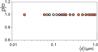
Figure 1: (Color online) Excluded volume simulations. Semi-log plot of the normalized theoretical self diffusion coefficient $\displaystyle D/D_{0}$ (open circles) computed according to Yoshida (1985) compared to the outcomes of the standard computation (filled squares) given by [Eqs.(21) and (34)] versus the average distance between the particles with vanishing intermolecular potential.

We considered hard-spheres with vanishing intermolecular potential, $\displaystyle U=0$, and modeling impenetrability as follows: whenever two molecules $\displaystyle i$ and $\displaystyle j$ get in touch and interpenetrate at some time $\displaystyle t$ (that is $\displaystyle|\boldsymbol{r}_{i}(t)-\boldsymbol{r}_{j}(t)|<2R$, with $\displaystyle R$ the radius of each molecule) we get back to $\displaystyle t-h$ and redraw the $\displaystyle\boldsymbol{\xi}_{i}(t)$ until $\displaystyle\boldsymbol{r}_{i,j}(t)$ are such that the impenetrability condition is satisfied. In Figure 1 we can see that the excluded volume effects on diffusion coefficient $\displaystyle D$ normalized with the Brownian value $\displaystyle D_{0}$ are very small. These results agree with the theoretically predicted values Yoshida (1985) according to which $\displaystyle D=D_{0}[1-2\phi]$ where $\displaystyle\phi=1/6\pi R^{3}n$ and $\displaystyle n=N/L^{3}$ is the number density.

III.2 Effects of long and short range electrostatic interactions at fixed average intermolecular distance

The next step is obtained by switching on interparticle interactions, keeping fixed all the parameters (temperature, viscosity, average interparticle distance, Debye length) but the number of charges $\displaystyle Z$. This way, we can vary only the intensity of the interparticle forces measuring the largest Lyapunov exponent and how $\displaystyle D$ deviates from Brownian motion. To begin with, the screened Coulomb potentials defined in Eq.(9) have been considered for an average intermolecular distance $\displaystyle\langle d\rangle=0.04\mu\text{m}$ and a Debye length $\displaystyle\lambda_{D}=0.01\mu\text{m}$. In Figure 2 and in Figure 3, we report the outcomes of these numerical simulations.

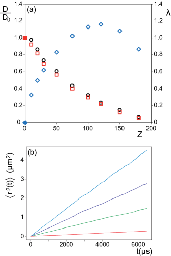
Figure 2: (Color online) (a) Normalized self diffusion coefficient $\displaystyle D/D_{0}$ (circles) computed according to [Eq.(29)] compared to the outcomes of the standard computation (squares) according to [Eqs.(21) and (34)] versus the number of charges $\displaystyle Z$ of the particles interacting through Coulomb potential with $\displaystyle\lambda_{D}=0.01\mu\text{m}$ [Eq.(9)] at average interparticle distance $\displaystyle\langle d\rangle=0.04\mu\text{m}$. On the second axes we report the largest Lyapunov exponent [Eq.(33)] (rhombus). Full symbols represent the corresponding theoretical values for vanishing $\displaystyle Z$ value. (b) Plot of the time evolution of the simulated MSD for different values of charge. The charge $\displaystyle Z$ increases starting from the top line that corresponds at $\displaystyle Z=10$, passing to $\displaystyle Z=50$, to $\displaystyle Z=100$, up to the bottom line corresponding at $\displaystyle Z=180$.

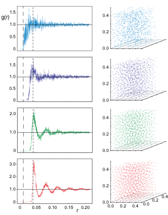
Figure 3: (Color online) Radial distribution function $\displaystyle g(r)$ [Eq.(35)] and particles position snapshots at the final simulation time for four charge values of Figure 2 starting from the top with $\displaystyle Z=10$ on the first line, $\displaystyle Z=50$ on the second line, $\displaystyle Z=100$ on the third line and $\displaystyle Z=180$ on the last one. Large dashed black line correspond to $\displaystyle r=\lambda_{D}=0.01\mu\text{m}$ while short dashed black line correspond to the $\displaystyle r=\langle d\rangle=0.04\mu\text{m}$. Full black line show the value $\displaystyle g(r)=1$. In the left panels the units of $\displaystyle r$ are $\displaystyle\mu\text{m}$, as well as the units of the snapshots axes to the right.

In Figure 2(a) we can see that the stronger the interparticle interaction the larger the deviation from the Brownian diffusion, that is stronger decrease of the diffusion coefficient $\displaystyle D$. The degree of chaoticity, represented by the largest Lyapunov exponent, is also affected by the strength of the interparticle interaction. At the same time, the time dependence of the MSD remains linear, that is, the chaotic diffusion still follows the Einstein-Fick law Crisanti et al. (1991), as it can be seen in Figure 2(b). The decreasing of the diffusion coefficient occurring in presence of repulsive interactions is due to the fact that the molecules uniformly fill all the accessible volume, thus, since there is no room for a free expansion of the system, the motion of any given molecule is somewhat hindered and slowed down by the surrounding ones. On the contrary, in presence of repulsive forces an increase of diffusion is expected when measured by mutual diffusion coefficient Tracy and Pecora (1992). The latter describes the decay of a concentration fluctuation and it is intuitive that under the action of repulsive forces a local higher density of particle diffuses faster than a Brownian diffusion. We can also observe a strikingly good agreement between the values of $\displaystyle D$ obtained through the time dependence of the MSD and by computing the theoretical corrections to Brownian value $\displaystyle D_{0}$ due to deterministic forces, according to Equation (29). The behavior of the Lyapunov exponents (Figure 2(a)) is characterized by an initial increase of the chaoticity of the system with a bending - towards lower values - beginning around $\displaystyle Z=120$. Such results can be qualitatively understood with the aid of the radial distribution functions $\displaystyle g(r)$ reported in Figure 3. The higher $\displaystyle Z$, the larger the range of spatial ordering as indicated by a larger numbers of peaks displayed by the function $\displaystyle g(r)$ at distance values which are multiples of the average intermolecular distance. The pattern of $\displaystyle g(r)$ with peaks oscillating around $\displaystyle 1$ is characteristic of a liquid and we can observe a transition from a gaseous-like state of the system for $\displaystyle Z=10$, to a short range order between $\displaystyle Z=50$ and $\displaystyle Z=100$, up to a long-range order for $\displaystyle Z=180$. We can surmise that the behavior of the LLE is due to the competition between the chaotic dynamics and the spatial ordering. To better elucidate this phenomenology, we have considered the unscreened Coulomb potential.

The results reported in Figures 4 and 5 have been obtained by means of the Coulomb potential defined in Eqs.(10) and (19) having kept constant all the parameters (as above with $\displaystyle\langle d\rangle=0.04\mu\text{m}$) with the exception of the number of charges $\displaystyle Z$.

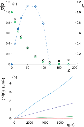
Figure 4: (Color online) (a) Normalized self diffusion coefficient $\displaystyle D/D_{0}$ (black circles) computed according to [Eq.(29)] compared to the outcomes of the standard computation (grey/green circles) according to [Eqs.(21) and (34)] versus the number of charges $\displaystyle Z$ of the particles interacting through a pure Coulomb potential [Eq.(10)] at average interparticle distance $\displaystyle\langle d\rangle=0.04\mu\text{m}$. On the second axes we report the largest Lyapunov exponent [Eq.(33)] (rhombus). Full symbols represent the corresponding theoretical values for vanishing $\displaystyle Z$ value. (b) Plot of the time evolution of the simulated MSD for different values of charge. The charge $\displaystyle Z$ increases starting from the top line that corresponds at $\displaystyle Z=10$, passing to $\displaystyle Z=50$, to $\displaystyle Z=100$, up to the bottom line corresponding at $\displaystyle Z=180$.

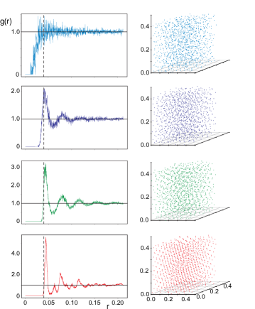
Figure 5: (Color online) Radial distribution function $\displaystyle g(r)$ [Eq.(35)] and particles position snapshots at the final simulation time for four charge values of Figure 4 starting from the top with $\displaystyle Z=10$ on the first line, $\displaystyle Z=50$ on the second line, $\displaystyle Z=100$ on the third line and $\displaystyle Z=180$ on the last one. Short dashed black line correspond to the $\displaystyle r=\langle d\rangle=0.04\mu\text{m}$. Full black line show the value $\displaystyle g(r)=1$. In the left panels the units of $\displaystyle r$ are $\displaystyle\mu\text{m}$, as well as the units of the snapshots axes to the right.

Likewise to Figure 2, we can observe that the stronger the interparticle interaction, the larger the deviation from Brownian diffusion, with a linear time dependence of the MSD for all the charge values used in these simulations, as shown in Figure 4(b). The increase of the strength of chaos, measured by Lyapunov exponents, observed between $\displaystyle Z=10$ and $\displaystyle Z=50$ (Figure 4(a)) is related to the increase of the strength of intermolecular interactions. This corresponds to a gaseous-like state of the system as shown by the first panel of Figure 5. In the second panel of the same Figure, the maximum value reached by the LLE, at $\displaystyle Z=50$, is attained when a sufficient degree of spatial order sets in so that it competes with dynamical chaos of the gaseous-like phase. The strong decrease of the LLE observed from $\displaystyle Z=75$ is due to a further enhancement of spatial order, as shown by the $\displaystyle g(r)$ in the third panel of Figure 5. The fourth panel of the same Figure shows a crystal-like arrangement of the molecules confirmed by the pattern of the function $\displaystyle g(r)$ Allen and Tildesley (1989). Moreover for $\displaystyle Z\geq 120$ the LLE drops to values very close to zero with a pattern displaying a seemingly sharp transition. Correspondingly, the diffusion coefficient also drops to zero after a monotonous decrease from its Brownian value at $\displaystyle Z=0$. Finally, the values of $\displaystyle D/D_{0}$ given by Eq.(29), reported in Figure 4(a), are again in very good agreement with the outcome of the standard computation; a growing discrepancy is observed in the above mentioned transition occurring at $\displaystyle Z=120$ where the degree of chaoticity is close to vanishing.

III.3 Effects of long and short range electrostatic interactions at fixed charge value

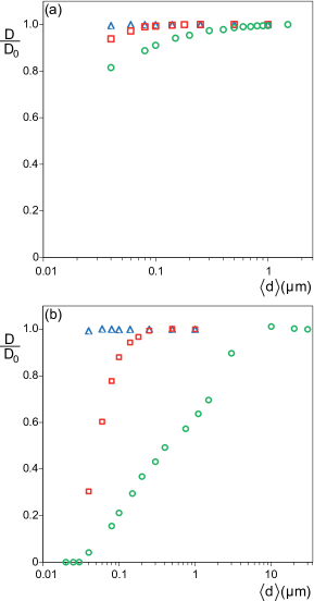
Figure 6: (Color online) Semi-log plot of the normalized self-diffusion coefficient $\displaystyle D/D_{0}$ versus the average distance of the particles interacting through Coulomb potentials [Eqs.(10) and (19)] for different combinations of $\displaystyle\lambda_{D}$ values at $\displaystyle Z=10$ (panel(a)) and $\displaystyle Z=100$ (panel (b)). The symbols indicate the Debye length values: $\displaystyle\lambda_{D}=0.001\mu\text{m}$ correspond to triangles, $\displaystyle\lambda_{D}=0.01\mu\text{m}$ to squares and $\displaystyle\lambda_{D}=\infty$ to circles.

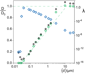
Figure 7: (Color online) Semi-log plot of the normalized self-diffusion coefficient versus the average distance of the particles interacting through Coulomb potential [Eqs.(19)] with $\displaystyle Z=100$. The normalized self diffusion coefficient $\displaystyle D/D_{0}$ (black circles) computed according to [Eq.(29)] is compared to the outcomes of the standard computation (grey/green circles) according to [Eqs.(21) and (34)]. On the second axes we report the largest Lyapunov exponent [Eq.(33)] (rhombus). The dashed lines are guides to the eye.

Let us now consider the effect of changing the interaction strength resulting from a variation of the average intermolecular distance and a variation of the action radius of electrostatic forces. This is obtained by using different Debye lengths ($\displaystyle\lambda_{D}=0.001$ and $\displaystyle 0.01\ \mu\mathrm{m}$) for the screened Coulomb potential defined in Eq.(9) and by using the Coulomb potential defined in Eqs. (10) and (19) ($\displaystyle\lambda_{D}=\infty$), for different charge values ($\displaystyle Z=10$ and $\displaystyle Z=100$).

The choice of these parameter values is partially inspired, on the one side, by the typical range of values of charges for proteins and for small fragments of nucleic acids, and, on the other side, the lowest value $\displaystyle\lambda_{D}=0.001\ \mu\mathrm{m}$ is approximately the Debye length of the cytosol while longer Debye lengths are relevant for prospective in vitro experiments. Figure 6 summarizes the dependence of the normalized mean diffusion coefficient as a function of the average distance among the molecules. Different values of $\displaystyle\lambda_{D}$ are considered for $\displaystyle Z=10$ (Fig.6 (a)) and $\displaystyle Z=100$ (Fig.6 (b)). We can observe that at low concentrations diffusion reaches its Brownian limit characterized by $\displaystyle D/D_{0}\simeq 1$, and the larger the Debye length and the number of charges, the larger the decrease of the diffusion coefficient. It turns out that an appreciable change in the diffusion coefficient shows up for $\displaystyle\lambda_{D}\geq 0.01\mu\text{m}$. The outcomes of numerical computations obtained for $\displaystyle Z=100$ and $\displaystyle\lambda_{D}=\infty$ are reported also in Figure 7 and compared with the values of the LLE and of the outcomes of the theoretical correction to the Brownian diffusion coefficient ((29)). At very high dilutions corresponding to an average interparticle distance larger than $\displaystyle 10\ \mu\mathrm{m}$, the diffusion is Brownian while at shorter interparticle distances the effect of electrostatic interactions is again a decrease of the diffusion coefficient up to a concentration corresponding to $\displaystyle\langle d\rangle=0.03\ \mu\mathrm{m}$ where diffusion stops. By resorting to the computation of the radial distribution functions we observe the same phenomenology reported in Figure 5, that is, in the case of Brownian diffusion the corresponding radial distribution function closely resembles to that in first panel of Figure 5. When diffusion deviates from being purely Brownian the radial distribution shows regular peaks as in the second and third panel of Figure 5 and it looks like that in the forth panel of Figure 5 when diffusion stops. At the same time, we observe an increase of the LLE which corresponds to the decrease of $\displaystyle D$ up to the point where $\displaystyle D$ vanishes. When $\displaystyle D$ vanishes, a sudden drop of the LLE is observed to practically zero values. Finally, we observe a very good agreement of the theoretical correction to the Brownian diffusion coefficient except when diffusion stops; this suggests that a developed chaoticity of the dynamics is a requisite for such a computation to be reliable.

III.4 Long range attractive dipolar effects

As remarked in the Introduction, we are interested in verifying the experimental detectability of long-range interactions among molecules of biological interest through their diffusive behavior. In this Section, we focus on the study of diffusive and dynamical properties of the system when both electrostatic Debye potential, described in Eq.(9), and attractive dipole-dipole electrodynamic potential, described in Eqs. (11) and (20), are involved. The choice of considering the simultaneous presence of these two kinds of interactions is motivated by the fact that biomolecules are charged objects with non-vanishing dipolar moments.

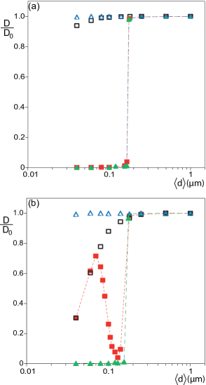
Figure 8: (Color online) Semi-log plot of the normalized self-diffusion coefficient $\displaystyle D/D_{0}$ versus the average distance of the particles interacting only through Coulomb potential [Eq.(10)] and through Coulomb potential and the attractive dipole-dipole potential [Eq.(20)] for different combinations of $\displaystyle\lambda_{D}$ values at $\displaystyle Z=10$ (panel (a)) and $\displaystyle Z=100$ (panel (b)). The symbol shapes indicate the Debye length values, $\displaystyle\lambda_{D}=0.001\mu\text{m}$ correspond to triangles and $\displaystyle\lambda_{D}=0.01\mu\text{m}$ to squares, while open symbols represent Coulomb potential and full ones the combined action of Coulomb and dipole-dipole potentials.

The dynamical properties and diffusive behavior in presence of an attractive interaction are qualitatively different from those observed in the previous sections regarding only the repulsive Coulomb potential. For the sake of clarity, we present and compare the combined presence of Coulomb and dipole-dipole electrodynamic potentials (represented by full symbols) with the presence of only Coulomb potential (represented by open symbols), the latter already presented in the previous Section. The kind of symbol corresponds, as before, to the different Debye length values: triangles correspond to $\displaystyle\lambda_{D}=0.001\ \mu\mathrm{m}$ and squares to $\displaystyle\lambda_{D}=0.01\ \mu\mathrm{m}$. In Figure 8 the numerical outcomes for the normalized diffusion coefficient, $\displaystyle D/D_{0}$, are reported as a function of the average intermolecular distance for two charge values, $\displaystyle Z=10$ (Fig. 8(a)) and $\displaystyle Z=100$ (Fig. 8(b)) and different values of the Debye lengths, both in presence and in absence of dipole-dipole electrodynamic potential. At very high dilutions, in a range between $\displaystyle\langle d\rangle=1\mu m$ and $\displaystyle\langle d\rangle=0.2\mu m$ the diffusion follows its Brownian limit characterized by $\displaystyle D/D_{0}\simeq 1$ for each combination of charge or potential as observed in both panels of the aforementioned figure. Let us resume first the results when only Coulomb potential is involved; in order to observe a significant deviation from the Brownian limit the Debye length must be at least equal to $\displaystyle 0.01\ \mu\mathrm{m}$ (open squares) with a more pronounced effect for $\displaystyle Z=100$ where the deviation from Brownian motion reaches $\displaystyle D/D_{0}\simeq 0.3$. To begin with, we switch on the dipolar potential focusing on the lower charge value, $\displaystyle Z=10$ (Fig. 8(a)). We can observe a sharp decrease of the normalized diffusion coefficient, with a transition between a diffusive Brownian motion and an absence of diffusion.

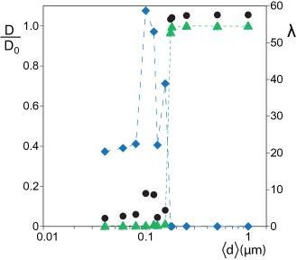
Figure 9: (Color online) Semi-log plot of the normalized self-diffusion coefficient versus the average distance of the particles interacting through Coulomb and dipolar potential [Eqs.(10) and (20)] with $\displaystyle Z=100$ and $\displaystyle\lambda_{D}=0.001\mu\text{m}$. The normalized self-diffusion coefficient $\displaystyle D/D_{0}$ (circles) computed according to [Eq.(29)] is compared to the outcomes of the standard computation (triangles) according to [Eqs.(21) and (34)]. On the second axes we report the largest Lyapunov exponent [Eq.(33)] (rhombus).

These results are independent of the action radius of Coulomb potential, in fact no difference has been observed between the two different Debye length values. The results reported in Figure 8(b)) are obtained by switching on the dipolar potential and by increasing the intensity of Coulomb potential (taking $\displaystyle Z=100$). When the Coulomb interactions is weak ($\displaystyle\lambda_{D}=0.001\ \mu\mathrm{m}$ full triangle), so that the dipolar contribution overcomes it, we can observe the same aforementioned sharp transition characterized by no diffusion. On the contrary, with a larger Debye length ($\displaystyle\lambda_{D}=0.01\ \mu\mathrm{m}$ full square) the effects of a competition between the two potentials, repulsive and attractive respectively, are observed when the average intermolecular distance is varied. At large average intermolecular distances the particle motions are practically independent one from the other resulting in a Brownian diffusion, while at shorter distances the mutual interactions play an important role. The interplay between the repulsive and attractive interactions leads to a diffusion behavior dominated by the dipolar interactions in a small range of distances in correspondence of the transition from $\displaystyle D/D_{0}\simeq 1$ to $\displaystyle D/D_{0}\simeq 0$, as it is observed in Figure 8(a). At smaller values of $\displaystyle\langle d\rangle$, the dipolar effect on diffusion is balanced by the presence of short-range Coulomb repulsion, thus preventing the formation of a clustered system. In Figure 9, we report the outcomes of numerical computations of $\displaystyle D/D_{0}$ versus $\displaystyle\langle d\rangle$ obtained in the case of a dominant dipolar potential with respect to the Coulomb one ($\displaystyle Z=100$ and Debye length $\displaystyle\lambda_{D}=0.001\ \mu m$). In the same figure, we add to $\displaystyle D/D_{0}$, the values of the LLE and of the outcomes of the theoretical correction to the Brownian diffusion coefficient due to interparticle interactions (Eq. (29)). This figure shows a good agreement between the theoretical correction to $\displaystyle D_{0}$ and the numerical results. We can also observe that the transition from a diffusive to a non-diffusive behavior goes with a sharp increase of the LLE, indicating a transition from a non-chaotic to a chaotic dynamics. Note that, in the transition region, fluctuating patterns of the LLE and of the theoretical correction to $\displaystyle D_{0}$ are found. We can surmise that in this region, since the dynamics displays long transients to the final clustered configurations, some memory of the initial conditions could be kept. In Figure 10 the radial distribution functions of the particles and the snapshots of their positions are given. These results refer to two average interparticle distances and confirm a transition from a gaseous-like state to a clustered configuration.

Finally, let us note that the results presented in the current Section indicate a possibility to disentangle the effects of electrostatic and electrodynamic interactions. In fact, by using a sufficiently high ion concentration in prospective experiments, and so weakening the electrostatic forces, only the effects of electrodynamic interactions would be observed.

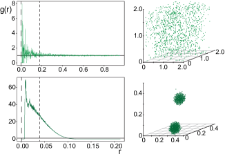
Figure 10: (Color online) Radial distribution function $\displaystyle g(r)$ [Eq.(35)] and particles position snapshots at the final simulation time at two average interparticle distance $\displaystyle\langle d\rangle=0.18\mu\text{m}$ (first line) and $\displaystyle\langle d\rangle=0.04\mu\text{m}$ (second line) for particles of $\displaystyle Z=100$ interacting with a Coulomb potential [Eq.(10) with $\displaystyle\lambda_{D}=0.001\mu\text{m}$] and with a dipolar potential [Eq.(20)]. The large dashed black line corresponds to $\displaystyle r=\lambda_{D}$ while short dashed black line corresponds to the $\displaystyle r=\langle d\rangle$. The full black line shows the value $\displaystyle g(r)=1$. In the left panels the units of $\displaystyle r$ are $\displaystyle\mu\text{m}$, as well as the units of the snapshots axes to the right.

IV Concluding remarks

As already stated in the Introduction, the present work is the sequel of a recent one aimed at assessing the experimental possibility of detecting long-range electrodynamic interactions between biomolecules. At variance with the outcomes of the previous work, the substantial advance provided by the present one consists of a conceptual proof of feasibility of an experimental approach resorting to an actually measurable observable. In particular, this observable is the diffusion coefficient that can be measured by means of several available techniques like pulsed-field gradient nuclear magnetic resonance forced Rayleigh scattering (FRS), Fluorescence Recovery After Photobleaching (FRAP) and Fluorescence Correlation Spectroscopy (FCS) to mention some of them. The long-range electrodynamic forces we are after have been hitherto elusive to observation in spite of many studies on the diffusion behavior of biomolecules in solution. We surmise that no evidence has been until now reported about the presence of these interactions because they are not compatible with thermal equilibrium Preto and Pettini (2013); Preto et al. contrary to previous predictions Fröhlich (1977). The consequence being the need for an out-of-equilibrium driving of the biomolecules by means of a source of collective excitation. In order to achieve the above mentioned assessment about experimental detectability of electrodynamic intermolecular interactions, we have performed numerical simulations whose outcomes can be summarized as follows:
i) We have found that, for dilute systems ($\displaystyle\langle d\rangle$ ranging from about $\displaystyle 400\mathrm{\AA}$ up to $\displaystyle 30000\mathrm{\AA}$ ), the diffusion coefficient is sensitive to all the interactions considered. Starting with a uniform distribution of molecules in all the accessible volume, an interesting phenomenon is observed: the diffusion coefficient decreases independently of the repulsive or attractive nature of the molecular interactions (repulsive Coulomb with and without screening, attractive electrodynamic dipole-dipole).
ii) Moreover, we observed that, in the gaseous-like phase, a decrease of the diffusion coefficient is always accompanied by an increase of chaos. On the contrary, when spatial order sets in, a decrease of the diffusion coefficient is always accompanied by a decrease of chaos. Even though it is well known that no simple relation exists between Lyapunov exponents and transport properties in dynamical systems, the qualitative correspondences observed are consistent with the intuitive idea that both phenomena are related to the intensity of intermolecular interactions.
iii) Nice transitional phenomena have been observed: for Coulomb interactions a first transition from purely stochastic diffusion to chaotic plus stochastic diffusion is found; then, at sufficiently high concentrations, a spatial ordering of the molecules is found resembling to a crystal-like structure. For dipole-dipole interactions an abrupt clustering transition is observed, which is strongly reminiscent of an equilibrium phase transition.
iv) The simple theoretical model proposed in Section II.5 gives the good values of the diffusion coefficients computed along the dynamics in presence of intermolecular interactions within a few percent of error. This result paves the way - at least in principle - to analytic predictions if the time averages used in this work are replaced by statistical averages Eq.(8) worked out with the Boltzmann-Gibbs weight Eq.(6) (which is the stationary measure associated with our model equations).
From the experimental point of view, which was the main motivation of the present work, we conclude that the variations of the diffusion coefficient $\displaystyle D$ with respect to its Brownian value, as well as the patterns of $\displaystyle D$ versus the average interparticle distance $\displaystyle\langle d\rangle$, are such that the practical possibility exists of experimentally tackling the problem of interest by means of, for example, one of the above mentioned techniques.