Study of the behaviour of proliferating cells in leukemia modelled by a system of delay differential equations

Abstract

For the model of periodic chronic myelogenous leukemia considered by Pujo-Menjouet, Mackey et al., model consisting of two delay differential equations, the equation for the density of so-called ”resting cells” was studied from numerical and qualitative point of view in several works. In this paper we focus on the equation for the density of proliferating cells and study it from a qualitative point of view.

Keywords: leukemia model, delay differential equations, qualitative analysis, stability, Hopf bifurcation, Bautin bifurcation.

1 Introduction

We consider the model of periodic chronic myelogenous leukemia consisting in the system of two delay differential equations [7], [8]:

$$\quad\frac{dP(t)}{dt}=-\gamma P(t)+\beta(N(t))N(t)-\frac{k}{2}\beta(N(t-r))N(t-r),$$

$$\frac{dN(t)}{dt}=-\left[\beta(N)+\delta\right]N(t)+k\beta(N(t-r))N(t-r).$$

Here $P(t)$ represents the density of proliferating cells while $N(t)$ is the density of so-called “resting” cells.

The function $\beta$ is given by $\displaystyle\beta(N)=\beta_{0}\theta^{n}/(\theta^{n}+N^{n}),\,n>0,$ and represents the rate at which the resting cells re-enter the proliferating phase.

For the detailed description of the model see [7]. We just remind that $\gamma>0$ is the rate of death of proliferating cell by apoptosis, $k=2e^{-\gamma r},$ $\delta>0$ is the rate by which the resting cells transform into normal cells, $\beta_{0}>0$ is the maximal rate of cell movement from the resting phase into proliferation; $\theta$ is the density of resting cell population such that $\beta(\theta)=\beta_{0}/2.$ The delay $r$ refers to a processus of division of the proliferation cells that takes place at time $r$ after they entered into the proliferating phase [7].

With $x(t)=P(t)/\theta,\,\,y(t)=N(t)/\theta$ the system becomes:

$$\;\;\;\;\;\;\;\dot{x}(t)=-\gamma x(t)+\frac{\beta_{0}y(t)}{1+y(t)^{n}}-\frac{k}{2}\frac{\beta_{0}y(t-r)}{1+y(t-r)^{n}},$$ (1)

$$\dot{y}(t)=-\left[\frac{\beta_{0}}{1+y(t)^{n}}+\delta\right]y(t)+k\frac{\beta_{0}y(t-r)}{1+y(t-r)^{n}}.$$ (2)

We see that the equation for $y$ does not depend on $x$. It was studied, from a numerical point of view in [7], [8], and from a qualitative point of view in [3], [4], [5] (in all these works, the density of resting cells,denoted here by $y$, was denoted by $x$). More precisely, in [3], the authors studied in depth the stability of the two equilibria of equation (2), in [4] the stability of periodic solution emerged by Hopf bifurcation was considered, while in [5] the existence of Bautin type bifurcation points was established.

Here we consider the first equation, that for the proliferating cells. Since their increase is the cause of the illness, the physician should be interested in the behaviour of $x(t)$ more than in that of $y(t)$. The equation for $x$ is very simple, it is a linear forced equation, with the forcing term depending on $y$. Hence the behaviour of $x$ is determined by that of $y$ (in the absence of the terms containing $y$, $x(t)$ would tend to zero when $t\rightarrow\infty$).

In the study of eq. (2), ([3], [4], [5]) in the zone of parameters that we considered (see Section 4) we encountered the following typical behaviours of $y$:

• $y(\cdot)$ is an equilibrium solution of (2), i.e. $y(t)=ct$;

• $y(t)$ tends to an equilibrium solution of (2), when $t$ tends to $\infty$;

• $y(\cdot)$ is a periodic solution of (2);

• $y(t)$ tends to a periodic solution of (2), when $t$ tends to $\infty$.

In the present paper, by using the results obtained on $y(\cdot)$, we study the behavior of $x(\cdot)$.

In the Appendix we prove some propositions that show how the behaviour of $y$ influences that of $x$. These are used in all the main sections of the paper.

In Section 2 we discuss the stability of the equilibria of eq. (1), indicating the zone of the parameters space where these are stable. Section 3 refers to the occurrence of Hopf bifurcation for $y$, that induces a similar behaviour for $x$. Section 4 refers to the Bautin bifurcation of $y$, that was studied in [5] and to its influence on $x$.

A section of Conclusions summarizes all the results in the paper.

2 Equilibria of the system, their stability

The system (1) - (2) has the equilibria: $x_{1}=0,\;\;y_{1}=0,$ and

$$x_{2}=\frac{2-k}{2\gamma}\frac{\beta_{0}y_{2}}{1+y_{2}^{n}},\;\;y_{2}=\left(\frac{\beta_{0}}{\delta}(k-1)-1\right)^{1/n}.$$

In this section we study the stability of these equilibria, by using the stability results contained in [3]. Let us remind that $y(\cdot),$ the solution of (2), is a bounded function, defined on $[-r,\,\infty)$, as shown in [3].

2.1 Stability of ($x_{1}$, $y_{1}$)

We intend to establish the stability of $(x_{1},\,y_{1})=(0,\,0)$ depending on the parameters of the problem. For this we shall use the results on the stability of $y$ in [3] and the results in the Appendix.

Propopsition 2.1. If

$$\frac{\beta_{0}}{\delta}(k-1)<1,$$ (3)

then the equilibrium solution $(x_{1},\,y_{1})$ of system (1), (2) is asymptotically stable.

Proof. By determining the set of parameters for which all eigenvalues of the linear equation attached to the delay differential equation (2) have negative real parts, in [3] it is shown that the solution $y_{1}=0$ of eq. (2) is asymptotically stable when $\frac{\beta_{0}}{\delta}(k-1)<1$.

Hence, in the same set of parameters, if the initial function $\phi\in\mathcal{C}([-r,0],\,\mathbb{R})$ for equation (2) is close enough to the function $y_{1}(s)=0,\,s\in[-r,0]$ such that the corresponding solution, $y(t,\,\phi)$ tends to $0$ when $t\rightarrow\infty,$ Proposition A.1 of the Appendix implies that $\displaystyle\lim_{t\rightarrow\infty}x(t)=0.$

It follows that the equilibrium solution $(x_{1},\,y_{1})$ of system (1), (2) is asymptotically stable.$\Box$

If we think at eq. (1) as a nonautonomous equation (and not a part of an autonomous system), in the conditions of the above Proposition, and if $\phi\in\mathcal{C}([-r,0],\,\mathbb{R})$ is such that $\lim_{t\rightarrow\infty}y(t,\phi)=0,$ then the solution $x_{1}=0$ of (1) is globally asymptotically stable.

Proposition 2.2. For $\frac{\beta_{0}}{\delta}(k-1)=1,$ the solution $(x_{1},\,y_{1})$ of system (1), (2) is stable.

Proof. When $\frac{\beta_{0}}{\delta}(k-1)=1,$ there is an eigenvalue, $\lambda,$ of the linearized eq. in $y$, that has $\mathrm{Re}\lambda=0$ [3]. In this situation, also in [3], we proved that there is a Lyapunov function for eq. (2), hence the solution $y_{1}=0$ is stable.

Now we prove that the solution $(x_{1},\,y_{1})$ of the system is stable. In eq. (1), we denote the terms containing $y$ by $F(y(t),\,y(t-r)):=\widetilde{F}(y)(t)$.

For this we consider an $\varepsilon>0$ and chose a $\delta_{\varepsilon}>0$ with the property that $|\phi|_{0}<\delta_{\varepsilon}$ implies $|y(t,\,\phi)|<\min\left(\frac{\varepsilon\gamma}{2\beta_{0}},\,\varepsilon\right)$, for any $t\geq 0$. This is possible due to the results in [3].

Then we have:

$$-\frac{\varepsilon\gamma}{2}<\frac{\beta_{0}y(t)}{1+y(t)^{n}}-\frac{k}{2}\frac{\beta_{0}y(t-r)}{1+y(t-r)^{n}}<\frac{\varepsilon\gamma}{2},\,\,\mathrm{for}\,\,t\geq T_{\varepsilon}.$$

Since the solution of equation (1) is

$$x(t,x_{0})=x_{0}e^{-\gamma t}+e^{-\gamma t}\int_{0}^{t}e^{\gamma s}\widetilde{F}(y)(s)ds,$$

relation (8) implies, for $t\geq T_{\varepsilon},$

$$|x(t,x_{0})|\leq|x_{0}|e^{-\gamma t}+e^{-\gamma t}\int_{0}^{t}e^{\gamma s}\frac{\varepsilon\gamma}{2}ds=$$

$$=|x_{0}|e^{-\gamma t}+(1-e^{-\gamma t})\frac{\varepsilon}{2}<|x_{0}|+\frac{\varepsilon}{2}.$$

Now, for $|x_{0}|\leq\frac{\varepsilon}{2},$ and $t\geq 0,$ we have

$$|x(t,x_{0})|\leq\varepsilon,$$

and since $|y(t,\,\phi)|<\varepsilon$ the solution $(0,\,0)$ of system (1), (2) is stable.$\Box$

Again, if we think at eq. (1) as a nonautonomous equation, in the conditions of Proposition 2.2, and if the initial condition of (2), $\phi\in\mathcal{C}([-r,0],\,\mathbb{R}),$ is close enough to $y_{1}=0$, then the solution $x_{1}=0$ of (1) is stable.

Proposition 2.3. When $\frac{\beta_{0}}{\delta}(k-1)>1$, the solution $(x_{1},\,y_{1})$ is unstable.

Proof. The condition $\frac{\beta_{0}}{\delta}(k-1)>1$ is the condition of existence of the equilibrium $y_{2}$ of (2). In [3] we proved that, in this situation, the solution $y_{1}$ loses stability (becomes unstable), hence the solution $(x_{1},\,y_{1})$ is also unstable.$\Box$

2.2 Stability of ($x_{2}$, $y_{2}$)

In the study of stability of $y_{2}$, [3], an important role is played by the constant $B_{1}=\frac{d}{dy}\left(\frac{\beta_{0}y}{1+y^{n}}\right)\left|{}_{y=y_{2}}\right.$ that occurs in the linearized of eq. (2). In fact, the linearized around $x_{2}$ of equation (2) is

$$\dot{z}(t)=-[B_{1}+\delta]z(t)+kB_{1}z(t-r),$$ (4)

and the value of $B_{1}$, in terms of the parameters of the problem is

$$B_{1}=\frac{\delta}{k-1}\left[\frac{n\delta}{\beta_{0}(k-1)}-n+1\right].$$ (5)

Proposition 2.4. If the following conditions are fulfilled:

• $B_{1}<0,$   ($\Leftrightarrow\displaystyle\frac{\beta_{0}}{\delta}(k-1)>\frac{n}{n-1}$);

• $\delta+B_{1}<0,$ ($\Leftrightarrow n>k\;and\;\displaystyle\frac{\beta_{0}}{\delta}(k-1)>\frac{n}{n-k}$);

• $|\delta+B_{1}|<|kB_{1}|$ and   $\displaystyle\frac{\arccos{((\delta+B_{1})/kB_{1})}}{\omega_{0}}<r<\frac{1}{|\delta+B_{1}|},$ where $\omega_{0}$ is the solution in $(0,\pi/r)$ of the equation $\omega\cot(\omega r)=-(\delta+B_{1});$

then, the solution $(x_{2},\,y_{2})$ of system (1), (2) is asymptotically stable.

Proof. As shown in [3], the conditions in the enounce are sufficient in order that all the eigenvalues of (4) have negative real part. That is, in these conditions, the solution $y_{2}$ is asymptotically stable.

For the initial condition $\phi\in\mathcal{C}([-r,0],\mathbb{R})$ in a small neighborhood of $y_{2}$, such that $\lim_{t\rightarrow\infty}y(t,\phi)=y_{2}$, Proposition A.1 implies that $\lim_{t\rightarrow\infty}x(t,x_{0})=x_{2}$, for any initial value $x_{0}$. It follows that $(x_{2},\,y_{2})$ is asymptotically stable.$\Box$

Proposition 2.5. If the following conditions are fulfilled:

• $B_{1}<0$ and $\delta+B_{1}>0,$ ($\Leftrightarrow\displaystyle\frac{n}{n-1}<\frac{\beta_{0}}{\delta}(k-1)<\frac{n}{n-k}$);

• $\delta+B_{1}>|kB_{1}|\,\,\mathrm{or}\,\left\{\delta+B_{1}\leq|kB_{1}|\,\,and\,\,\displaystyle r<\frac{\arccos{((\delta+B_{1})/kB_{1})}}{\omega_{0}}\right\}$ with $\omega_{0}$ defined as above;

then the solution $(x_{2},\,y_{2})$ of system (1), (2) is asymptotically stable.

Proof. Again, the results in [3] show that $y_{2}$ is asymptotically stable in the conditions of the enounce. This and Proposition A.1 imply that, for the initial function $\phi$ of eq. (2) in a convenient neighborhood of $y_{2}$, we have $x(t)\rightarrow x_{2}$ when $t\rightarrow\infty$, hence the equilibrium $x_{2}$ of equation (1) is (globally) asymptotically stable, and the equilibrium $(x_{2},\,y_{2})$ of system (1), (2) is asymptotically stable.$\Box$

If we consider eq. (1) as a non-autonomous differential equation, if either the conditions of Proposition 2.4 or those of Proposition 2.5 are satisfied and if $\phi$ is such that $\lim_{t\rightarrow\infty}y(t,\phi)=y_{2}$, then $x_{2}$ is a globally asymptotically stable equilibrium of (1).

Proposition 2.6. If $B_{1}>0$, then the solution $(x_{2},\,y_{2})$ of system (1), (2) is asymptotically stable.

Proof. As proved in [3], for $B_{1}>0$, $y_{2}$ is asymptotically stable. This implies (via Proposition A.1) the asymptotic stability of $(x_{2},\,y_{2})$ as solution of eq. (1), (1).$\Box$

As above, we remark, that, if $\phi$ is such that $\lim_{t\rightarrow\infty}y(t,\phi)=y_{2}$, then $x_{2}$ is a globally asymptotically stable equilibrium of (1).

3 Points of Hopf bifurcation for $y$.
Influence on $x$

The analysis in [7], [8], [4] shows that the equilibrium $y_{2}$ loses stability by a Hopf bifurcation, at points where $B_{1}<0$ and

$$r=\frac{\arccos{((\delta+B_{1})/kB_{1})}}{\sqrt{(kB_{1})^{2}-(\delta+B_{1})^{2}}}.$$ (6)

Propositions A.1, A.2 and A.3 show that, when the delayed differential equation (2) presents a Hopf bifurcation, the solutions of equation in $x$ behave like having a Hopf bifurcation (because of the term in $y$).

Indeed, for the zone of stability of $y_{2}$, we already saw that $x(t,\,x_{0})\rightarrow x_{2},$ when $t\rightarrow\infty$, for any $x_{0}\geq 0$.

After the Hopf bifurcation, an attractive periodic orbit occurs for the equation in $y$. This implies, as Propositions 2.2 and 2.3 show, that there is a certain initial value $\widetilde{x}_{0}=\widetilde{u}_{0}+x_{2}$ such that $x(t,\widetilde{x}_{0})$ is a periodic orbit in the phase portrait of eq. (1), orbit that is asymptotically stable.

Hence, in the points from the parameters space where $y(\cdot)$ presents Hopf bifurcation, the function describing the density of proliferating cells, $x(\cdot)$, behaves like having a Hopf bifurcation also. Of course it is not a genuine Hopf bifurcation, since the eigenvalue of the linearized equation in $x$ at $x_{2}$ is $-\gamma$, it is only a behaviour induced by the “forcing term” $\widetilde{F}(y)$.

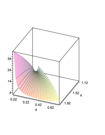
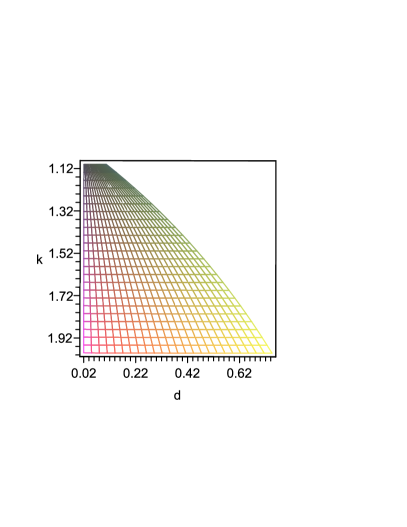
Figure 1: Left- Surface of Hopf bifurcation points in the $(\delta,\,k,\,r)$ space ($n=2$, $\beta_{0}=2.5$). Right- Projection of the surface on the plane $(k,\,\delta)$. Here $\delta$ is denoted by $d$.

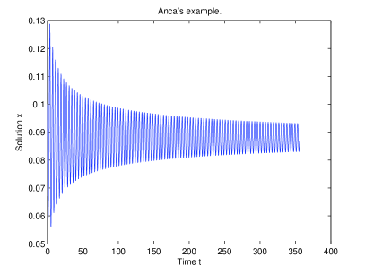
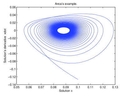
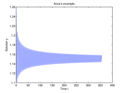
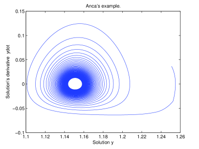
Figure 2: Left- $x(t)$ versus $t$ before the Hopf bifurcation point, at $r=0.3558$. Right- $\dot{x}(t)$ versus $x(t)$ at $r=0.3558$.

Figure 3: Left- $y(t)$ versus $t$ before the Hopf bifurcation point, at $r=0.3558$. Right- $\dot{y}(t)$ versus $y(t)$ at $r=0.3558$.

In order to have an image of the points in the parameters space where this happens, we fix two parameters, $n$ and $\beta_{0}$ and in the three dimensional space of the other parameters, $(k,\,\delta,\,r)$, we represent $r$ as function of $(k,\,\delta)$, by using (6). In Fig. 1 such a plot, for $n=1,\,\beta_{0}=2.5$, can be seen, together with the projection of this surface on the $(k,\,\delta)$ plane (representing the domain of definition of the function in (6)).

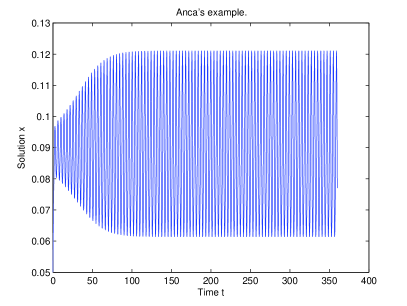
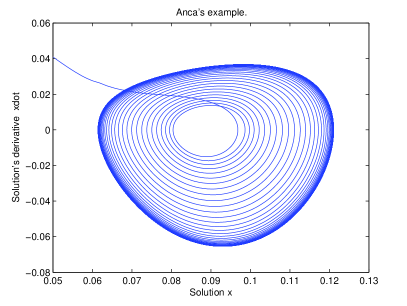
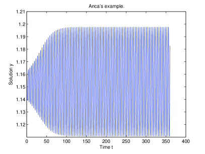
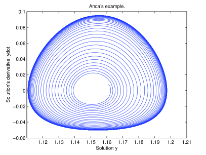
Figure 4: Left- $x(t)$ versus $t$ after the Hopf bifurcation point, at $r=0.36$. Right- $\dot{x}(t)$ versus $x(t)$ at $r=0.36$.

Figure 5: Left- $y(t)$ versus $t$ after the Hopf bifurcation point, at $r=0.36$. Right- $\dot{y}(t)$ versus $y(t)$ at $r=0.36$.

As a matter of fact, condition (6) is only a necessary condition for Hopf bifurcation and it must be completed with the condition that the first Lyapunov coefficient, $l_{1}$, is different of zero (for the definition of $l_{1}$ see [4], where the restriction of the problem to a center manifold is used). If $l_{1}=0$, then depending on the number of varying parameters, either a Hopf degenerate bifurcation (a single varying parameter) or a Bautin bifurcation (two varying parameters) takes place.

In Figures 2, 3, 4, 5, we present the solutions $x(t)$ and $y(t)$ at a typical Hopf bifurcation point, ($n=12,\,\beta_{0}=1.77,\,\delta=0.05,\,k=1.18074,\,r=0.3559114$). Here $r$ was taken the bifurcation parameter. Figures 2 and 3 present the solutions, for the parameter $r$ at the left of the bifurcation value (at $r=0.3558$) while Figures 4 and 5 present the solutions, for $r$ at the right of the bifurcation value ($r=0.36$). It is clear that the behaviour of $y$ determines that of $x$. We remark that the first Lyapunov coefficient for this Bautin bifurcation is $l_{1}=-43.71.$

4 Points of Bautin bifurcation for $y$.
Influence on $x$

In [5] we studied the Bautin bifurcation for eq. (2). The Bautin bifurcation occurs when $l_{1}=0$ and the second Lyapunov coefficient, $l_{2}$, is different of zero. For the definition of $l_{2}$ see [5] - where again the problem is restricted to a two-dimensional center manifold. By this restriction a two dimensional system of differential equations is obtained. For this kind of problems, the Bautin bifurcation was studied in [6].

In the Bautin bifurcation two parameters are varied, hence we may speak of a parameters plane and the normal form of this bifurcation in polar coordinates is

$$\dot{\rho}=\rho(b_{1}+b_{2}\rho^{2}+\zeta\rho^{4}),$$

$$\dot{\theta}=1,$$

where $\zeta=\mathrm{sgn}(l_{2}).$

The Bautin bifurcation is characterized by the fact that, if we vary the parameters in the parameters plane, around the bifurcation point, we can meet four possible situations. These are, as can be seen on the bifurcation diagram, Fig. 6: an equilibrium point (in the domain denoted by 1 of the parameters plane), an equilibrium surrounded by a limit cycle (in domain 2), an equilibrium surrounded by two cycles one inside the other (zone 3), and, finally, an equilibrium that is attracting on one side and repelling on its other side (for points on the curve T). The curve T is the curve on which the discriminant of equation $b_{1}+b_{2}\eta+\zeta\eta^{2}=0$ is equal to zero and the solution $\eta$ is positive (since $\eta=\rho^{2}$).

The stability properties of the trajectories described above depend on the sign of $l_{2}$, as we can see in the bifurcation diagrams (Fig. 6).

The letter “H” on the bifurcation diagram shows that, while crossing the vertical axis, in the sense indicated by the small arrows, Hopf bifurcation takes place.

Figure 6: Bautin bifurcation diagram. Left- the case $l_{2}<0$; Right- the case $l_{2}>0$.

The algorithm for finding Bautin bifurcation points for eq. (2) was described in detail in [5]. We only shortly remind the results of our search.

We considered the zone of parameters $(n,\,\beta_{0},\,k)$ given by:

$$(n,\,\beta_{0},\,k)\in\{1,1.5,2,3,...,12\}\times\{0.5,1,1.5,2,2.5\}\times\{1.1,1.2,...,1.9\}$$

(we remind that $k>1$ in order that $x_{2}$ exist, and $k<2$). $(n,\beta_{0},k)$ were taken as fixed parameters, and $(\delta,\,r)$ as variable parameters. Hence, for every $(n^{*},\beta^{*}_{0},k^{*})$ fixed, we looked for a $\delta^{*}$ and a $r^{*}$ such that $Re\lambda_{1,2}(\alpha^{*})=0$ and $l_{1}(\alpha^{*})=0,$ where we denoted by $\alpha$ the vector of parameters, $\alpha=(n,\,\beta_{0},\,k,\,\delta,\,r)$.

For $\mathbf{n=1}$ we showed [5] that the condition (6) for Hopf bifurcation is not satisfied, hence no Bautin bifurcation can occur.

For $\mathbf{n=1.5}$ and $\mathbf{n=2},$ and for each $\beta_{0}\in\{0.5,\,1,\,1.5,\,2,\,2.5\},$ and each $k\in\{1.1,\,1.2,...,1.9\}$ we found Hopf points with $l_{1}=0$. For these points we computed the second Lyapunov coefficient and found that for each of the bifurcation points obtained, $l_{2}<0$. Hence they are Bautin bifurcation points and the bifurcation diagram is that of Fig. 6, left.

For $\mathbf{3\leq n\leq 12}$ and $\beta_{0}\in\{0.5,\,1,\,1.5,\,2,\,2.5\},$ $k\in\{1.1,\,1.2,...,1.9\}$, the first Lyapunov coefficient was find to be always negative, hence, no Bautin bifurcation is possible for this range of parameters.

We give, below, the points, found by us, in the parameters space where $l_{1}=0$ for the case $n=2$ and $\beta_{0}\in\{0.5,\,1,\,1.5,\,2\}$ and $k$ as above. Also we present the plots of these Bautin bifurcation points on the surfaces of Hopf points (Figs. 7 - 10). By connecting these points, we obtain approximate curves of Bautin bifurcation points on the surfaces of Hopf points.

A table and a figure of the same type, for the case $n=2,\,\beta_{0}=2.5$, were published in [5].

k	$\delta$	$r$	$l_{2}$
1.1	0.0045705962	26.125314	-0.021
1.2	0.0090491351	25.751524	-0.0151
1.3	0.0134437887	25.422162	-0.0124
1.4	0.0177612407	25.130258	-0.0108
1.5	0.0220070315	24.870352	-0.0097
1.6	0.0261858065	24.638093	-0.0088
1.7	0.0303014988	24.429962	-0.0081
1.8	0.0343574676	24.243076	-0.0076
1.9	0.0383566021	24.075039	-0.0071

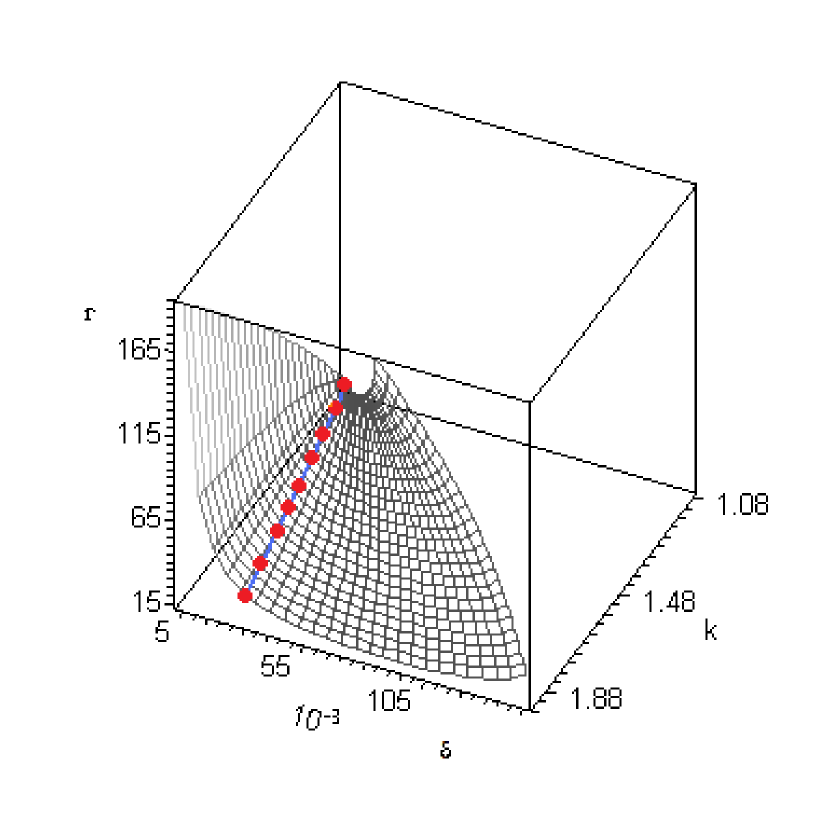
Figure 7: Hopf codimension two points for $n=2,\,\beta_{0}=0.5.$

k	$\delta$	$r$	$l_{2}$
1.1	0.0091411924	13.062657	-0.0205
1.2	0.0180982702	12.875762	-0.0142
1.3	0.0268875774	12.711081	-0.0114
1.4	0.0355224814	12.565129	-0.0097
1.5	0.0440140630	12.435176	-0.0085
1.6	0.0523716129	12.319046	-0.0076
1.7	0.0606029975	12.214981	-0.0069
1.8	0.0687149345	12.121538	-0.0063
1.9	0.0767132043	12.037519	-0.0059

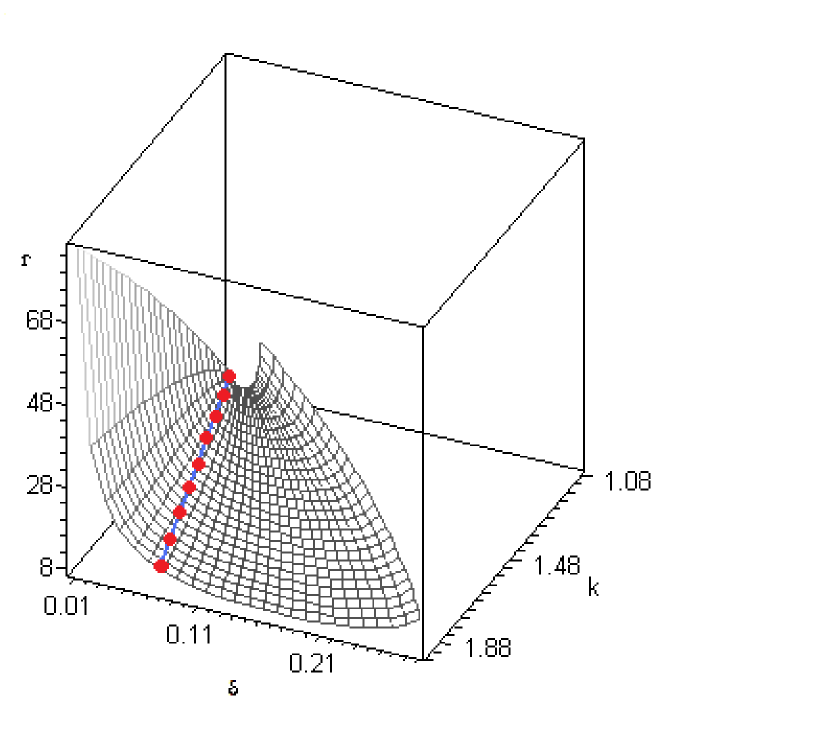
Figure 8: Hopf codimension two points for $n=2,\,\beta_{0}=1.$

k	$\delta$	$r$	$l_{2}$
1.1	0.0137117887	8.708438	-0.0204
1.2	0.0271474053	8.583841	-0.0140
1.3	0.0403313662	8.474054	-0.0112
1.4	0.0532837222	8.376752	-0.0095
1.5	0.0660210946	8.290117	-0.0083
1.6	0.0785741932	8.212697	-0.0074
1.7	0.0909044966	8.143320	-0.0067
1.8	0.1030724022	8.081025	-0.0061
1.9	0.1150698062	8.025013	-0.0056

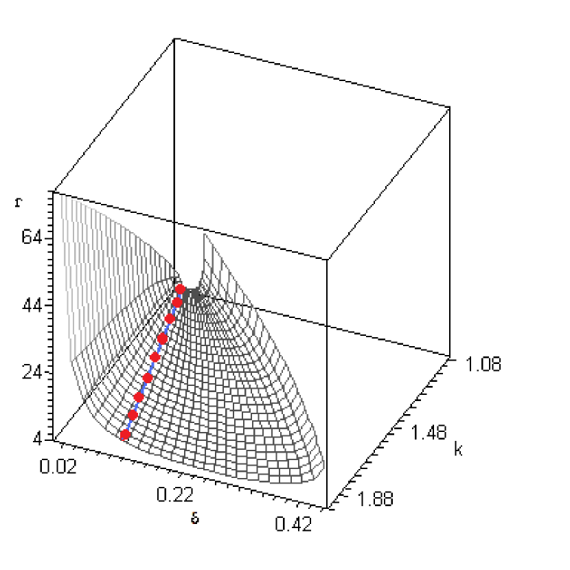
Figure 9: Hopf codimension two points for $n=2,\,\beta_{0}=1.5.$

k	$\delta$	$r$	$l_{2}$
1.1	0.018282385	6.531328	-0.0203
1.2	0.036196540	6.437880	-0.014
1.3	0.053775154	6.355540	-0.0111
1.4	0.071044963	6.282564	-0.0093
1.5	0.088028126	6.217588	-0.0082
1.6	0.104743225	6.159523	-0.0073
1.7	0.121205995	6.107490	-0.0066
1.8	0.137429869	6.060769	-0.0060
1.9	0.153426408	6.018759	-0.0055

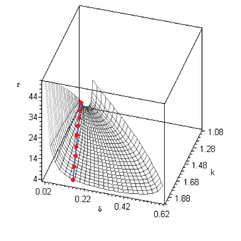
Figure 10: Hopf codimension two points for $n=2,\,\beta_{0}=2.$

In [5], in order to confirm by numerical integration the behaviour predicted by the bifurcation diagram, we considered a Bautin bifurcation point $P^{*}$, identified by the algorithm in [5], at $n^{*}=2,\,\beta^{*}_{0}=2.5,$ $k^{*}=1.01,\,$ and $r^{*}=5.301432998$, $\delta^{*}=0.0023073665$.

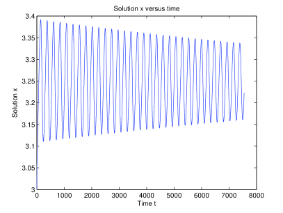
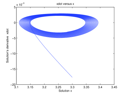
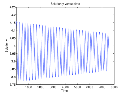
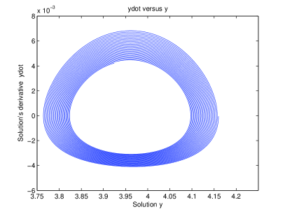
Figure 11: Graphs of $x(\cdot),$ respectively $y(\cdot)$, for point $P_{3},\;\;c=0.2$ .

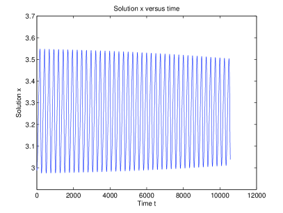
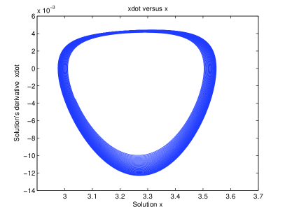
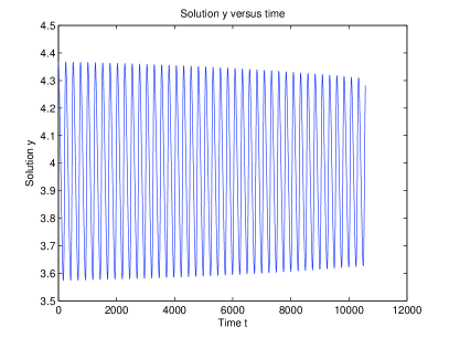
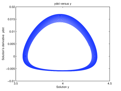
Figure 12: Graphs of $x(\cdot),$ respectively $y(\cdot)$, for point $P_{3},\;\;c=0.41$ .

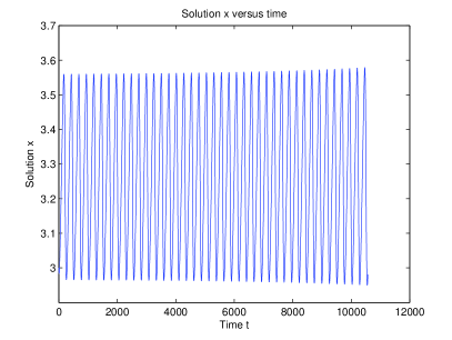
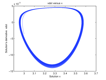
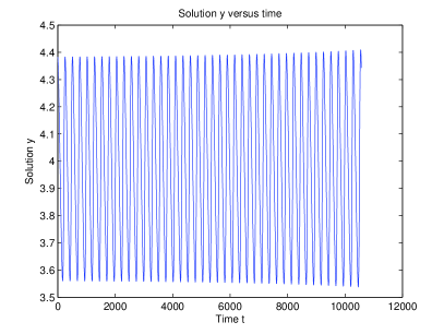
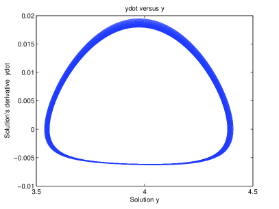
Figure 13: Graphs of $x(\cdot),$ respectively $y(\cdot)$, for point $P_{3},\;\;c=0.425$ .

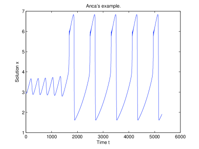
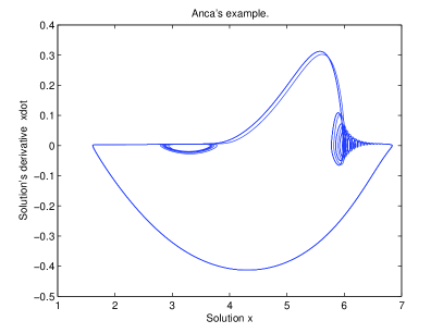
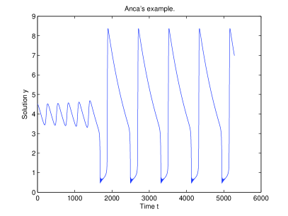
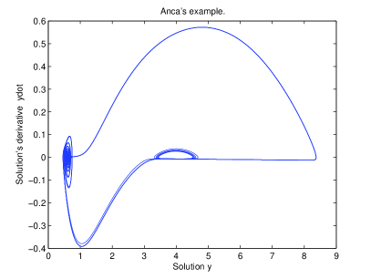
Figure 14: Graphs of $x(\cdot),$ respectively $y(\cdot)$, for point $P_{3},\;\;c=0.55$.

In the present paper, for the same point, $P^{*}$, we show, in parallel, the behaviour of $y$ and that of $x$ for the parameters chosen in the (most interesting) zone, corresponding to the zone 3 of the bifurcation diagram (Fig. 6, left). There, for $y$, two limit cycles exist (one inside the other), the inner cycle being unstable while the outer one, stable. By numerical investigations, we found that point $P_{3}(7.55,\,0.0015)$ lies in this zone. For this point, the second equilibrium of system (1), (2) is $x_{2}=3.24777,\,y_{2}=3.95811$.

As initial function $y_{0}=\phi$, for eq. (2), we considered functions of the type $\phi(s)=y_{2}+ce^{\mu s}\cos(\omega s),\,s\in[-r,0]$, where $\lambda_{1,2}=\mu\pm i\omega$ are the two eigenvalues with greatest real part corresponding to the chosen parameters. Hence the parameter $c$ determines the distance between the initial function $\phi$ and the equilibrium $y_{2}.$

Depending on $c$, the orbit $y(t,\phi)$ will either tend towards $y_{2}$ (being rejected by the unstable inner limit cycle) or towards the outer limit cycle. First we take $c=0.2,$ and $c=0.41$ and see that $y(t)$ tend towards $y_{2}$ and $x(t)$ tends to $x_{2}$ (Figs 11 and 12). For $c=0.425$ the oscillating orbits have increasing amplitude (Fig. 13). It is clear that between $c=0.41$ and $c=0.425$ there must be a value $c^{*}$ such that for the initial function $\phi^{*}(s)=y_{2}+c^{*}e^{\mu s}\cos(\omega s),\,s\in[-r,0]$, the corresponding solution $y(t,\phi^{*})$ of eq. (2) is a periodic function. This is the unstable periodic orbit (inner limit cycle on the center manifold) of the equation for $y$.

We notice that for $c=0.425$ the amplitude of the orbits increases very slowly. If we take a greater value of $c$, e.g. $c=0.55,$ for a short interval of time, the amplitude increases slowly, and then there is a sudden increase of the amplitude, and the solution rapidly tends to a periodic orbit, that is stable (Fig. 14). This one corresponds to the outer limit cycle from the center manifold. This behaviour of $y$ is reproduced, qualitatively, by $x$, as is seen in Figure 14.

5 Conclusions

In this paper we investigated the behaviour of the solution $x$ of the system (1), (2), the function $x$ representing the nondimensional density of proliferating cells in the leukemia disease. It is seen that the behaviour of $x$ is determined by that of $y$ (density of resting cells).

We studied the stability of the equilibrium solutions, and we presented the conditions that the parameters should satisfy, in order that the equilibrium solutions $x_{1},\,x_{2}$ of eq. (1) be stable or even globally asymptotically stable.

Then, we establish the conditions on the parameters such the solution $x$ mimics a Hopf bifurcation (i.e. the equilibrium loses stability and a stable periodic orbit occurs).

The third type of interesting behaviour of $y$ previously studied [5] is the Bautin bifurcation. We showed that, when $y$ presents some Bautin bifurcation, the solution $x$ also mimics this kind of bifurcation.

The study concerning the Bautin bifurcation is important because, for parameters in the domains corresponding to the domain 3 of the bifurcation diagram, the behaviour of $x$ may have two very different aspects. That is $x(t)$ may tend to $x_{2}$ or to the periodic orbit that corresponds to the outer limit cycle of the reduced to the center manifold problem for $y$. The initial value of $x$ is irrelevant in deciding what behaviour $x$ has. Only the initial function for $y$ matters.

We also provide tables and figures with points of Bautin bifurcation space for $n=2$ and $\beta_{0}\in\{0.5,\,1,\,1.5,\,2\},$ $k\in\{1.1,\,1.2,...,1.9\}$. The conclusions presented for the occurrence or non-occurrence of Bautin bifurcation, refer to an important zone of the parameters space, that is $1\leq n\leq 12$ and $\beta_{0},\,k$ as above.

The investigation may be extended to other parameters zones by using the method exposed in [5].

More than that, we also performed numerical integrations that confirm the qualitative behaviours that we theoretically predicted - Figs. 2-5 and Figs. 11-14.

Remark. We remark once more that, for all considered problems: stability, Hopf bifurcation or Bautin bifurcation, the long time behaviour of $x$ does not depend on the initial condition for this function ($x(0)=x_{0}$), but depends on the initial state of the function $y$.

This is important for the physician or for the biologist, because it shows that, in order to make a long time prediction on the development of the illness, the initial value of $y$, that is of the function that models the ”resting cells” should be known and not that of $x$. As an example, in Figures 11-14, for the same parameters, depending on the initial condition of $y$, $x(t)$ tends either to $x_{2}$ or to a large stable periodic orbit. The initial value of $x(\cdot)$ may only influence the length of the time interval in which $x(t)$ approaches its asymptotic behaviour, determined by $y$.

In the Appendix we prove some (simple) results that show how $y$ detemines $x$.

6 Appendix

We assert and prove some results that are necessary in the study of the main part of the paper.

In order to present the results in an unified form, we make the following notations. We denote by $(x^{*},\,y^{*})$ one of the two equilibria $(x_{1},\,y_{1})$ or $(x_{2},\,y_{2})$. Remind that we denoted the terms containing $y$ from eq. (1), by $\widetilde{F}(y)(t)$, such that eq. (1) takes the form

$$\frac{dx}{dt}(t)=-\gamma x(t)+\widetilde{F}(y)(t).$$

If $y^{*}=y_{2},$ we rewrite eq. (1) as

$$\frac{d(x-x_{2})}{dt}=-\gamma(x-x_{2})+\frac{\beta_{0}y(t)}{1+y(t)^{n}}-\frac{\beta_{0}y_{2}}{1+y_{2}^{n}}-\frac{k}{2}\left(\frac{\beta_{0}y(t-r)}{1+y(t-r)^{n}}-\frac{\beta_{0}y_{2}}{1+y_{2}^{n}}\right).$$

We set $u=x-x_{2},\;\;$ and the equation becomes

$$\frac{du}{dt}(t)=-\gamma u(t)+\widetilde{F}(y)(t)-\widetilde{F}(y_{2}).$$

We denote

$$H(y)(t):=\left\{\begin{array}[]{ll}\widetilde{F}(y)(t),&\hbox{if}\,\,\,y^{*}=y_{1},\\ \widetilde{F}(y)(t)-\widetilde{F}(y_{2}),&\hbox{if}\,\,\,y^{*}=y_{2},\end{array}\right.$$

and we see that in both situations above our equation has the form

$$\frac{du}{dt}(t)=-\gamma u(t)+H(y)(t),$$ (7)

where $H(y)(t)\rightarrow 0$ when $t\rightarrow\infty.$

Proposition 2.1. If $y(t)\rightarrow y^{*}$ when $t\rightarrow\infty$, then $x(t)\rightarrow x^{*}$ when $t\rightarrow\infty$.

Proof. We prove that $u(t)\rightarrow 0$ when $t\rightarrow\infty$. The solution, denoted $u(\cdot,\,u_{0})$, of the above equation with the initial condition $u(0)=u_{0}$, is

$$u(t,\,u_{0})=u_{0}e^{-\gamma t}+e^{-\gamma t}\int_{0}^{t}e^{\gamma s}H(y)(s)ds.$$ (8)

Let $\varepsilon>0$. Since $H(y)(t)\rightarrow 0$ there is a $T>0$ such that for $t>T,$ we have $|H(y)(t)|<\frac{\varepsilon\gamma}{3}$. Then we write, for $t\geq T,$

$$|u(t,u_{0})|\leq|u_{0}e^{-\gamma t}|+|e^{-\gamma t}\int_{0}^{T}e^{\gamma s}H(y)(s)ds|+|e^{-\gamma t}\int_{T}^{t}e^{\gamma s}H(y)(s)ds|\leq$$ (9)

$$\leq|u_{0}|e^{-\gamma t}+e^{-\gamma t}\int_{0}^{T}e^{\gamma s}|H(y)(s)|ds+e^{-\gamma t}\int_{T}^{t}e^{\gamma s}\frac{\varepsilon\gamma}{3}ds=$$

$$=|u_{0}|e^{-\gamma t}+e^{-\gamma t}\int_{0}^{T}e^{\gamma s}|H(y)(s)|ds+\frac{\varepsilon\gamma}{3}\frac{1}{\gamma}\left(1-e^{\gamma(T-t)}\right).$$

We chose a $T^{\prime}>T$ such that $|u_{0}|e^{-\gamma T^{\prime}}<\frac{\varepsilon}{3}$ and $e^{-\gamma T^{\prime}}\int_{0}^{T}e^{\gamma s}|H(y)(s)|ds<\frac{\varepsilon}{3}$.
Then, for any $t\geq T^{\prime}$, we have

$$|u(t,u_{0})|<\varepsilon,$$

and the conclusion follows. $\Box$

Proposition 2.2. If $y(\cdot)$ is periodic, there is a initial value $\widetilde{x}_{0}$ of eq. (1) such that the corresponding solution $x(\cdot,\,\widetilde{x}_{0})$ is periodic and it is asymptotically stable.

Proof. If $y(\cdot)$ is periodic, then the function $H(\cdot)$ of eq. (7) is periodic. Then, a classical result ([2], pg. 214) shows that there is an $\widetilde{u}_{0}$ such that the corresponding solution $u(\cdot,\,\widetilde{u}_{0})$ of eq. (7) is periodic.

We show that it is asymptotically stable. Let us consider another initial condition $u_{0}.$ The corresponding solution of (7) is

$$u(t,u_{0})=e^{-\gamma t}u_{0}+\int_{0}^{t}e^{\gamma(s-t)}H(y)(s)ds=$$

$$=e^{-\gamma t}\widetilde{u}_{0}+\int_{0}^{t}e^{\gamma(s-t)}H(y)(s)ds+e^{-\gamma t}(u_{0}-\widetilde{u}_{0})=$$

$$=u(t,\,\widetilde{u}_{0})+e^{-\gamma t}(u_{0}-\widetilde{u}_{0}),$$

since the sum of the first two terms is the solution of (7) corresponding to $\widetilde{u}_{0}$. It is clear that

$$\lim_{t\rightarrow\infty}|u(t,u_{0})-u(t,\,\widetilde{u}_{0})|=0,$$

that implies the asymptotic stability of the periodic solution.

The conclusions upon $u$ transfer to $x,$ q.e.d. $\Box$

Proposition 2.3. If $y(\cdot)$ tends to a periodic function when $t\rightarrow\infty$, then $x(t,y_{0})$ tends to a periodic orbit when $t\rightarrow\infty$.

Proof. Let $p:[0,\infty)\mapsto\mathbb{R}$ be a periodic function such that

$$\lim_{t\rightarrow\infty}|y(t)-p(t)|=0.$$

With the notation of the preceding Proposition, we see that $H(p)(\cdot)$ is periodic. We set $o(t)=H(y)(t)-H(p)(t)$.

It is not difficult to show that $\displaystyle\lim_{t\rightarrow\infty}o(t)=0.$

Now we write eq. (7) as

$$\dot{u}(t)=-\gamma u(t)+H(p)(t)+o(t)$$

that has solution

$$u(t,u_{0})=e^{-\gamma t}u_{0}+\int_{0}^{t}e^{\gamma(s-t)}H(p)(s)ds+\int_{0}^{t}e^{\gamma(s-t)}o(s)ds.$$

As we pointed out in the proof of Proposition 2.2, in [2] it is shown that there is an initial value $\widetilde{u}_{0}$ such that the function

$$e^{-\gamma t}\widetilde{u}_{0}+\int_{0}^{t}e^{\gamma(s-t)}H(p)(s)ds$$

is periodic. On the other hand, by a reasoning similar to that applied to the last term of (9), we prove that $\displaystyle\lim_{t\rightarrow\infty}\int_{0}^{t}e^{\gamma(s-t)}o(s)ds=0.$

It follows that for the initial condition $\widetilde{u}_{0},$ the solution $u(\cdot,\widetilde{u}_{0})$ tends to a periodic function. Now, for $u_{0}\neq\widetilde{u}_{0},$ we have

$$u(t)=e^{-\gamma t}u_{0}+\int_{0}^{t}e^{\gamma(s-t)}H(p)(s)ds+\int_{0}^{t}e^{\gamma(s-t)}o(s)ds=$$

$$=e^{-\gamma t}\widetilde{u}_{0}+\int_{0}^{t}e^{\gamma(s-t)}H(p)(s)ds+e^{-\gamma t}(u_{0}-\widetilde{u}_{0})+\int_{0}^{t}e^{\gamma(s-t)}o(s)ds.$$

Since the last two terms tend to zero when $t\rightarrow\infty,$ it again follows that $u(\cdot,u_{0})$ tends to a periodic function. Hence $x(\cdot,x_{0})$ has the same property.$\Box$

References

- [1] Adelina Georgescu, I. Oprea, Bifurcation theory from application viewpoint, Tipografia Univ. Timişoara, 1994, (Monografii Matematice 51).
- [2] A. Halanay, Qualitative theory of differential equations, Editura Academiei Republicii Populare Române, 1963. (in Romanian)
- [3] A. V. Ion, New results concerning the stability of equilibria of a delay differential equation modeling leukemia, Proceedings of The 12th Symposium of Mathematics and its Applications, Timişoara, November 5-7, 2009, 375-380; arXiv:1001.4658.
- [4] A. V. Ion, R. M. Georgescu, Stability of equilibrium and periodic solutions of a delay equation modeling leukemia, Works of the Middle Volga Mathematical Society, 11(2009); arXiv:1001.5354.
- [5] A. V. Ion, R.M. Georgescu, Bautin bifurcation in a delay differential equation modeling leukemia, Nonlinear Analysis, 82(2013), 142-157.
- [6] Y. A. Kuznetsov, Elements of applied bifurcation theory, Applied Mathematical Sciences, 112, Springer, New York, 1998.
- [7] L. Pujo-Menjouet, M. C. Mackey, Contribution to the study of periodic chronic myelogenous leukemia, C. R. Biologies, 327(2004), 235-244.
- [8] L. Pujo-Menjouet, S. Bernard, M. C. Mackey, Long period oscillations in a model of hematopoietic stem cells, SIAM J. Applied Dynamical Systems, 2, 4(2005), 312-332.