A combinatorial approach to the algebra of hypermatrices

Abstract.

We present two hypermatrix formulations of the Cayley–Hamilton theorem. One of the proposed formulation naturally extends to hypermatrices the combinatorial interpretations of the classical Cayley–Hamilton theorem. We conclude by discussing an application of the theorem to computing graph invariants which distinguish some non-isomorphic graphs with isospectral adjacency matrices.

1. Introduction.

The importance of a graph theoretical perspective to the algebra of matrices is well established[Zei85, RD08]. We show that insights provided by a combinatorial lens on the algebra of matrices also shed light on the algebra of multidimensional generalization of matrices called hypermatrices. Formally, a hypermatrix denotes a finite set of numbers whose distinct members are indexed by distinct elements of a Cartesian product set of the form

$$\left\{1,2,\cdots,n_{1}\right\}\times\left\{1,2,\cdots,n_{2}\right\}\times\cdots\times\left\{1,2,\cdots,n_{d}\right\}.$$

Such a hypermatrix is said to be of order $d$ and of size $n_{1}\times n_{2}\times\cdots\times n_{d}$. In particular matrices are second order hypermatrices. The algebra of hypermatrices arises from attempts to extend to hypermatrices familiar matrix algebra concepts [MB94, IGZ94, Ker08, GER11]. A survey of important hypermatix results can be found in [Lim13]. The discussion here mostly focuses on the Bhattacharya-Mesner (BM) hypermatrix algebra [MB90, MB94]. On occasion we also discuss the general BM product developed in [GER11, Gna14]. The general BM product has the benefit of encompassing as special cases many other hypermatrix products such as the Segre outer product, the contraction product and the multilinear matrix multiplication described in detailed in [Lim13]. Our main result are two new hypermatrix formulations of the Cayley–Hamilton theorem. The first of which extends to hypermatrices combinatorial interpretations of the classical Cayley–Hamilton theorem described in [RD08, Zei85], while the second formulation is distinctively less combinatorial and more algebraic. The second formulation has the benefit of bearing a close resemblance to the classical Cayley–Hamilton theorem. It also lends itself more easily to the computation of invariants. Finally we discuss an application of the hypermatrix formulations of the Cayley–Hamilton theorem to computing graph invariants which distinguish some non-isomorphic graphs whose adjacency matrices are isospectral.

Acknowledgement.

We would like to thank Andrei Gabrielov for providing guidance and inspiration while preparing this manuscript. We would like to thank Vladimir Retakh and Ahmed Elgammal for patiently introducing us to the theory of hypermatrices. We are grateful to Doron Zeilberger, Ha Luu and Sowmya Srinivasan for helpful discussions and suggestions. The author was supported by the the National Science Foundation, and is grateful for the hospitality of the Institute for Advanced Study.

2. Overview of the Bhattacharya-Mesner algebra

We recall here for convenience of the reader the basic elements of the Bhattacharya-Mesner (BM) algebra proposed in [MB90, MB94] as a generalization of the algebra of matrices.

Definition 1.

The Bhattacharya-Mesner [MB90, MB94] algebra generalizes the classical matrix product

$$\mathbf{B}=\mathbf{A}^{(1)}\cdot\mathbf{A}^{(2)}$$

where $\mathbf{A}^{(1)}$, $\mathbf{A}^{(2)}$, $\mathbf{B}$ are matrices of sizes $n_{1}\times k$, $k\times n_{2}$, $n_{1}\times n_{2}$, respectively,

$$b_{i_{1},i_{2}}=\sum_{1\leq{\color[rgb]{1,0,0}j}\leq k}a_{i_{1},{\color[rgb]{1,0,0}j}}^{(1)}\,a_{{\color[rgb]{1,0,0}j},i_{2}}^{(2)},$$

to an $m$-operand hypermatrix product noted

$$\mathbf{B}=\mbox{Prod}\left(\mathbf{A}^{(1)},\,\cdots,\mathbf{A}^{(m)}\right),$$

where $\mathbf{B}$ is an $n_{1}\times\cdots\times n_{m}$ hypermatrix, for $i=1,\cdots,\left(m-1\right)$, $\mathbf{A}^{(i)}$ is a hypermatrix whose size is obtained by replacing $n_{i+1}$ by $k$ in the dimensions of the hypermatrix $\mathbf{B}$, and $\mathbf{A}^{(m)}$ is a $k\times n_{2}\times\cdots\times n_{m}$ hypermatrix,

$$b_{i_{1},\cdots,i_{m}}=\sum_{1\leq{\color[rgb]{1,0,0}j}\leq k}a_{i_{1},{\color[rgb]{1,0,0}j},i_{3},\cdots,i_{m}}^{(1)}\cdots\,a_{i_{1},\cdots,i_{t},{\color[rgb]{1,0,0}j},i_{t+2},\cdots,i_{m}}^{(t)}\cdots\,a_{{\color[rgb]{1,0,0}j},i_{2},\cdots,i_{m}}^{(m)}.$$

In the particular case of third order hypermatrices, $\mathbf{A}^{(1)}$, $\mathbf{A}^{(2)}$, $\mathbf{A}^{(3)}$ and $\mathbf{B}$ are hypermatrices of sizes $n_{1}\times k\times n_{3}$, $n_{1}\times n_{2}\times k$, $k\times n_{2}\times n_{3}$ and $n_{1}\times n_{2}\times n_{3}$ respectively,

$$b_{i_{1},i_{2},i_{3}}=\sum_{1\leq{\color[rgb]{1,0,0}j}\leq k}a_{i_{1},{\color[rgb]{1,0,0}j},i_{2}}^{(1)}\,a_{i_{1},i_{2},{\color[rgb]{1,0,0}j}}^{(2)}\,a_{{\color[rgb]{1,0,0}j},i_{1},i_{2}}^{(3)}.$$

The general BM product was introduced in [GER11] and noted

$$\mathbf{C}=\mbox{Prod}_{\mathbf{B}}\left(\mathbf{A}^{(1)},\,\cdots,\mathbf{A}^{(m)}\right).$$

The hypermatrix $\mathbf{C}$ is an $n_{1}\times\cdots\times n_{m}$ hypermatrix, while the dimensions of the hypermatrix $\mathbf{A}^{(i)}$ for $i=1,\cdots,\>m-1$ is obtained by replacing $n_{i+1}$ by $k$ in the dimensions of $\mathbf{C}$ and $\mathbf{A}^{(m)}$ is a hypermatrix of size $k\times n_{2}\times\cdots\times n_{m}$ similarly to the BM product. Crucially, the general BM product differs from the BM product in the fact that the general product involves an additional input hypermatrix. The additional product input hypermatrix $\mathbf{B}$ is called the background hypermatrix and as such $\mathbf{B}$ must be a cubic $m$-th order hypermatrix having all of its sides of length $k$,

$$c_{i_{1},\cdots,i_{m}}=\sum_{1\leq{\color[rgb]{1,0,0}j_{1}},{\color[rgb]{1,0,0}j_{2}},{\color[rgb]{1,0,0}\cdots},{\color[rgb]{1,0,0}j_{m}}\leq k}a_{i_{1},{\color[rgb]{1,0,0}j_{2}},i_{3},\cdots,i_{m}}^{(1)}\cdots a_{i_{1},\cdots,i_{t},{\color[rgb]{1,0,0}j_{t+1}},i_{t+2},\cdots,i_{m}}^{(t)}\cdots a_{{\color[rgb]{1,0,0}j_{1}},i_{2},\cdots,i_{m}}^{(m)}\,b_{{\color[rgb]{1,0,0}j_{1}},{\color[rgb]{1,0,0}j_{2}},{\color[rgb]{1,0,0}\cdots},{\color[rgb]{1,0,0}j_{m}}}.$$

Note that the original BM product is recovered by setting $\mathbf{B}$ to the Kronecker delta hypermatrix (i.e. the hypermatrix whose nonzero entries all equal one and are located at the entries whose indices all have the same value, in particular Kronecker delta matrices are identity matrices).

3. Hypermatrix formulation of the Cayley–Hamilton theorem.

The classical Cayley–Hamilton theorem, establishes a tight upper bound for the dimension of the span of consecutive powers of a generic $n\times n$ matrix. While it is clear that the dimension of the span of consecutive Hadamard powers of a generic $n\times n$ matrix is $n^{2}$, it is surprising that the dimension of the span of consecutive powers of a generic $n\times n$ matrix is at most $n$. Similarly, hypermatrix formulations of the Cayley–Hamilton theorem establish tight upper bounds on the dimension of span of hypermatrix powers. Hypermatrix powers correspond to compositions of BM products.

3.1. First formulation of the Cayley–Hamilton theorem.

The first formulation of the Cayley–Hamilton theorem is based on the BM product introduced in [MB90, MB94]. Recall that the BM algebra is non associative. Consequently, the number of distinct compositions of product a cubic hypermatrix $\mathbf{A}$ is determined by the Fuss-Catalan numbers[Lin11]. In particular, a third order hypermatrix $\mathbf{A}$ admits the following three distinct fifth degree composition of product.

$$\mbox{Prod}\left(\mathbf{\mathbf{A}},\mathbf{A},\mbox{Prod}\left(\mathbf{A},\mathbf{A},\mathbf{A}\right)\right),$$

$$\mbox{Prod}\left(\mathbf{\mathbf{A}},\mbox{Prod}\left(\mathbf{A},\mathbf{A},\mathbf{A}\right),\mathbf{A}\right),$$

$$\mbox{Prod}\left(\mbox{Prod}\left(\mathbf{A},\mathbf{A},\mathbf{A}\right),\mathbf{\mathbf{A}},\mathbf{A}\right).$$

Note that the BM product noted $\mbox{Prod}\left(\mathbf{A},\mathbf{A},\mathbf{A}\right)$ corresponds to a third degree power. Furthermore third order hypermatrices admit by construction no even degree powers.

Theorem 2.

The dimension of the span of the vector space of third order cubic hypermatrix powers is maximal, that is equal to the number of hypermatrix entries.

For notational convenience, we restrict the discussion to third order hypermatrices, however the argument presented here naturally extends to hypermatrices of arbitrary order.

Proof.

We first observe each row-column slices of the powers of a generic third order hypermatrix $\mathbf{A}$, can be expressed as some matrix polynomial of the corresponding row-column slice of $\mathbf{A}$. Consequently the upper bound on the dimension of the span of powers of cubic hypermatrices of order $d$ and of side length $n$ is a fixed polynomial in $n$ noted $p_{d}\left(n\right)$. Furthermore the third order BM product is ternary, the number of distinct powers of degree $2k+1$ is determined by the recurrence formula

$$c_{3}=1,\quad c_{2k+1}=\sum_{0<i,j,i+j<2k+1}c_{i}\,c_{j}\,c_{2k+1-\left(i+j\right)}.$$ (3.1)

The recurrence 3.1 is a special case of the Fuss-Catalan numbers[Lin11] and in this particular case given by

$$c_{2n+1}=\frac{{3n\choose n}}{2n+1}.$$

as easily verified via the WZ method [PWZ96]. Furthermore, it is clear that $p_{3}\left(n\right)$ is a polynomial of degree at most $3$. Consequently by the polynomial argument it suffices to exhibit explicit constructions of four hypermatrices $\mathbf{A}_{0}$, $\mathbf{A}_{1}$, $\mathbf{A}_{2}$ and $\mathbf{A}_{3}$ of size $n_{0}\times n_{0}\times n_{0}$, $n_{1}\times n_{1}\times n_{1}$, $n_{2}\times n_{2}\times n_{2}$ and $n_{3}\times n_{3}\times n_{3}$ respectively such that

$$1\leq n_{0}<n_{1}<n_{2}<n_{3}$$

and most importantly, the span of the powers has maximal dimension.
Let $n_{0}=1$ and $\mathbf{A}_{0}$ be the third order hypermatrix expressed

$$\mathbf{A}_{0}=\left[a_{1,1,1}=1\right].$$

Let $n_{1}=2$ and $\mathbf{A}_{1}$ be determined by it’s row column $2\times 2$ matrix slices given by

$$\mathbf{A}_{1}\left[:,:,0\right]=\left(\begin{array}[]{cc}1&1\\ -1&1\end{array}\right),\quad\mathbf{A}_{1}\left[:,:,1\right]=\left(\begin{array}[]{cc}1&1\\ 1&1\end{array}\right).$$

Let $n_{2}=3$ and $\mathbf{A}_{2}$ be determined by it’s row column $3\times 3$ matrix slices given by

$$\mathbf{A}_{2}\left[\,:,\,:,\,0\right]=\left(\begin{array}[]{rrr}-1&-1&45\\ 0&-8&-1\\ 3&-79&1\end{array}\right),\,\mathbf{A}_{2}\left[\,:,\,:,\,1\right]=\left(\begin{array}[]{rrr}-3&-1&2\\ -49&10&-3\\ -6&2&-1\end{array}\right)$$

$$\mathbf{A}_{2}\left[\,:,\,:,\,2\right]=\left(\begin{array}[]{rrr}-1&2&-1\\ -1&-1&0\\ -1&0&-1\end{array}\right)$$

Finally, let $n_{3}=4$ and $\mathbf{A}_{3}$ be determined by it’s row column $4\times 4$ matrix slices given by

$$\mathbf{A}_{3}\left[\,:,\,:,\,0\right]=\left(\begin{array}[]{rrrr}2&0&2&-1\\ -3&1&1&2\\ 2&-1&1&6\\ -1&-3&0&20\end{array}\right),\,\mathbf{A}_{3}\left[\,:,\,:,\,1\right]=\left(\begin{array}[]{rrrr}0&0&-1&3\\ 0&-1&-20&-1\\ 2&1&2&-1\\ 3&-1&1&0\end{array}\right)$$

$$\mathbf{A}_{3}\left[\,:,\,:,\,2\right]=\left(\begin{array}[]{rrrr}1&1&0&-3\\ 0&1&0&1\\ 6&-1&-1&0\\ -2&-2&-5&2\end{array}\right),\,\mathbf{A}_{3}\left[\,:,\,:,\,3\right]=\left(\begin{array}[]{rrrr}-7&-2&-1&11\\ -1&-1&3&78\\ -3&3&0&-1\\ 9&0&0&2\end{array}\right).$$

One easily verifies for $\mathbf{A}_{0}$, $\mathbf{A}_{1}$, $\mathbf{A}_{2}$ and $\mathbf{A}_{3}$ that the dimension of the vector space spanned by the powers is respectively $1^{3}$, $2^{3}$, $3^{3}$ and $4^{3}$ respectively. This concludes the proof. ∎

Having established the maximality of the span, Cramer’s rule is used to express the rational functions of the hypermatrix entries associated with the linear dependence between of $n^{3}+1$ powers.

3.2. Second formulation of the Cayley–Hamilton theorem.

Recall that the matrix powers can be computed via a recurrence formula with initial conditions

$$\left\{\mathbf{A}^{[0]}=\boldsymbol{\Delta},\>\mathbf{A}^{[1]}=\mathbf{A}\right\}$$

where

$$\left[\boldsymbol{\Delta}\right]_{i,j}=\begin{cases}\begin{array}[]{cc}1&\mbox{ if }i=j\\ 0&\mbox{otherwise}\end{array}\end{cases},$$

and recurrence formula given by

$$\begin{cases}\begin{array}[]{ccc}\mathbf{A}^{[k+2]}&=&\mbox{Prod}_{\mathbf{A}^{[k]}}\left(\mathbf{A},\mathbf{A}\right)\\ \mathbf{A}^{[k+3]}&=&\mbox{Prod}_{\mathbf{A}^{[k+1]}}\left(\mathbf{A},\mathbf{A}\right)\end{array}\end{cases}.$$

Consequently, the classical Cayley–Hamilton theorem establishes the existence of sequence of rational functions

$$\left\{\alpha_{k}\left(a_{1,1},\cdots,a_{n,n}\right)\right\}_{0\leq k<n}\subset\mathbb{Q}\left(a_{1,1},\cdots,a_{n,n}\right)$$

such that

$$\mathbf{0}_{n\times n}=\mathbf{A}^{[n]}+\sum_{0\leq k<n}\mathbf{A}^{[k]}\,\alpha_{k}\left(a_{1,1},\cdots,a_{n,n}\right).$$

The second hypermatrix formulation of the Cayley–Hamilton theorem is also defined by the recurrence

$$\left\{\mathbf{A}^{[0]}=\boldsymbol{\Delta},\>\mathbf{A}^{[1]}=\mathbf{A}\right\}$$

where

$$\left[\boldsymbol{\Delta}\right]_{i,j,k}=\begin{cases}\begin{array}[]{cc}1&\mbox{ if }i=j=k\\ 0&\mbox{otherwise}\end{array}\end{cases},$$

and recurrence formula given by

$$\begin{cases}\begin{array}[]{ccc}\mathbf{A}^{[k+2]}&=&\mbox{Prod}_{\mathbf{A}^{[k]}}\left(\mathbf{A},\mathbf{A},\mathbf{A}\right)\\ \mathbf{A}^{[k+3]}&=&\mbox{Prod}_{\mathbf{A}^{[k+1]}}\left(\mathbf{A},\mathbf{A},\mathbf{A}\right)\end{array}\end{cases}.$$

Theorem 3.

The dimension of the span of the vector space of third order cubic hypermatrix powers in the sequence is maximal, that is equal to the number of hypermatrix entries.

The proof of the theorem is similar to the previous proof in that we observe each row-column slices of the powers of a generic third order hypermatrix $\mathbf{A}$, can be expressed as some matrix polynomial of the corresponding row-column slice of $\mathbf{A}$. Consequently the upper bound on the dimension of the span of powers of cubic hypermatrices of order $d$ and of side length $n$ is a fixed polynomial in $n$ noted $p_{d}\left(n\right)$.

Proof.

The proof is similar to the proof given in the first formulation. We describe hypermatrices $\mathbf{A}_{0}$, $\mathbf{A}_{1}$, $\mathbf{A}_{2}$ and $\mathbf{A}_{3}$ of size $n_{0}\times n_{0}\times n_{0}$, $n_{1}\times n_{1}\times n_{1}$, $n_{2}\times n_{2}\times n_{2}$ and $n_{3}\times n_{3}\times n_{3}$ respectively such that

$$1\leq n_{0}<n_{1}<n_{2}<n_{3}.$$

The powers, of hypermatrices the span of the powers has maximal dimension.
Let $n_{0}=1$ and $\mathbf{A}_{0}$ be the third order hypermatrix expressed

$$\mathbf{A}_{0}=\left[a_{1,1,1}=1\right].$$

Let $n_{1}=2$ and $\mathbf{A}_{1}$ be determined by its row column $2\times 2$ matrix slices given by

$$\mathbf{A}_{1}\left[:,:,1\right]=\left(\begin{array}[]{rr}-7&-7\\ 1&-1\end{array}\right),\quad\mathbf{A}_{1}\left[:,:,2\right]=\left(\begin{array}[]{rr}2&4\\ 1&-2\end{array}\right).$$

Let $n_{2}=3$ and $\mathbf{A}_{2}$ be determined by its row column $3\times 3$ matrix slices given by

$$\mathbf{A}_{2}\left[\,:,\,:,\,1\right]=\left(\begin{array}[]{rrr}-1&18&0\\ -3&0&5\\ 2&-1&2\end{array}\right),\,\mathbf{A}_{2}\left[\,:,\,:,\,2\right]=\left(\begin{array}[]{rrr}0&-5&-2\\ -3&1&1\\ 1&-2&0\end{array}\right)$$

$$\mathbf{A}_{2}\left[\,:,\,:,\,3\right]=\left(\begin{array}[]{rrr}-1&0&1\\ -1&2&-14\\ 6&-3&1\end{array}\right)$$

Finally, let $n_{3}=4$ and $\mathbf{A}_{3}$ be determined by its row column $4\times 4$ matrix slices given by

$$\mathbf{A}_{3}\left[\,:,\,:,\,1\right]=\left(\begin{array}[]{rrrr}18&0&0&1\\ 0&3&-1&-1\\ 0&52&4&5\\ -1&-1&-4&0\end{array}\right),\,\mathbf{A}_{3}\left[\,:,\,:,\,2\right]=\left(\begin{array}[]{rrrr}1&0&-2&8\\ -2&1&1&1\\ 4&-2&6&-2\\ -1&-1&1&-2\end{array}\right)$$

$$\mathbf{A}_{3}\left[\,:,\,:,\,3\right]=\left(\begin{array}[]{rrrr}10&-1&0&-1\\ 1&0&1&3\\ 1&-1&0&0\\ 0&1&13&-1\end{array}\right),\,\mathbf{A}_{3}\left[\,:,\,:,\,4\right]=\left(\begin{array}[]{rrrr}4&12&2&0\\ -1&-1&-3&1\\ -1&1&0&0\\ 155&-1&0&0\end{array}\right).$$

One easily verifies for $\mathbf{A}_{0}$, $\mathbf{A}_{1}$, $\mathbf{A}_{2}$ and $\mathbf{A}_{3}$ that the dimension of the vector space spanned by the powers is respectively $1^{3}$, $2^{3}$, $3^{3}$ and $4^{3}$ respectively. This concludes the proof. ∎

4. A combinatorial interpretation of the hypermatrix Cayley-Hamilton theorem.

Let $\mathbf{A}$ denote an $m\times n\times p$ third order hypermatrix. We associate with $\mathbf{A}$ a directed tripartite $3$-uniform hypergraph $H\left(\mathbf{A}\right)$. The hypergraph $H\left(\mathbf{A}\right)$ has $m$ vertices in the first partition, $n$ vertices in the second partition and $p$ vertices in the third partition. The vertices in the first, second and third partition are respectively colored red, green and blue. The vertex coloring scheme is designed to establish a one to one correspondence between entries of $\mathbf{A}$ and ( red, green, blue ) triplets of vertices in $H\left(\mathbf{A}\right)$. More precisely, the directed hyperedge spanning the $i$-th red vertex noted $\mbox{R}_{{\color[rgb]{1,0,0}i}}$, the $j$-th green vertex noted $\mbox{G}_{{\color[rgb]{0,1,0}j}}$ and the $k$-th blue vertex noted $\mbox{B}_{{\color[rgb]{0,0,1}k}}$, is associated with the $a_{{\color[rgb]{1,0,0}i},{\color[rgb]{0,1,0}j},{\color[rgb]{0,0,1}k}}$ hypermatrix entry. In short we say that $a_{{\color[rgb]{1,0,0}i},{\color[rgb]{0,1,0}j},{\color[rgb]{0,0,1}k}}$ is the weight of the $\left(\mbox{R}_{{\color[rgb]{1,0,0}i}},\mbox{G}_{{\color[rgb]{0,1,0}j}},\mbox{B}_{{\color[rgb]{0,0,1}k}}\right)$ hyperedge of $H\left(\mathbf{A}\right)$. The proposed directed tripartite hypergraph $H\left(\mathbf{A}\right)$ described here is a natural extension of the König directed bipartite graph associated with matrices described in [RD08].

4.1. Composing Hypergraphs.

By analogy to the matrix case, the König directed hypergraph yields a combinatorial interpretation of the BM product. The hypergraph composition is defined by the following vertex ( and induced edge ) identification scheme. Consider tripartite hypergrahs $H\left(\mathbf{A}^{(1)}\right)$, $H\left(\mathbf{A}^{(2)}\right)$, $H\left(\mathbf{A}^{(3)}\right)$ respectively associated with the $m\times t\times p$ hypermatrix $\mathbf{A}^{(1)}$, the $m\times n\times t$ hypermatrix $\mathbf{A}^{(2)}$ and the $t\times n\times p$ hypermatrix $\mathbf{A}^{(3)}$. Incidentally, the number of red vertices of $H\left(\mathbf{A}^{(1)}\right)$ equals the number of red vertices of $H\left(\mathbf{A}^{(2)}\right)$. Similarly the number of green vertices of $H\left(\mathbf{A}^{(2)}\right)$ also corresponds to the number of green vertices of $H\left(\mathbf{A}^{(3)}\right)$. Finally the number of blue vertices of $H\left(\mathbf{A}^{(1)}\right)$ equals the number of blue vertices of $H\left(\mathbf{A}^{(3)}\right)$. The size constraints, express the size requirement for the BM product of $\mathbf{A}^{(1)}$, $\mathbf{A}^{(2)}$, and $\mathbf{A}^{(3)}$. The result of the composition is a directed tripartite hypergraph associated with an $m\times n\times p$ hypermatrix. As suggested by the pairwise size constraints relating the hypergraph pair $\left(H\left(\mathbf{A}^{(1)}\right),H\left(\mathbf{A}^{(2)}\right)\right)$ the red vertices of $H\left(\mathbf{A}^{(1)}\right)$ are identified according to their label with the red vertices of $H\left(\mathbf{A}^{(2)}\right)$. Similarly, following the pairwise size constraints relating the hypergraph pair $\left(H\left(\mathbf{A}^{(2)}\right),H\left(\mathbf{A}^{(3)}\right)\right)$ the green vertices of the hypergraph $H\left(\mathbf{A}^{(2)}\right)$ are identified according to their label to the green vertices of the hypergraph $H\left(\mathbf{A}^{(3)}\right)$. Finally, following the pairwise constraints relating the hypergraph pair $\left(H\left(\mathbf{A}^{(1)}\right),H\left(\mathbf{A}^{(3)}\right)\right)$ the blue vertices of $H\left(\mathbf{A}^{(1)}\right)$ are identified according to their label with the blue vertices of $H\left(\mathbf{A}^{(3)}\right)$. The final step of the identification consists in identifying vertices of different colors according to their labels. Namely remaining green vertices of $H\left(\mathbf{A}^{(1)}\right)$, the blue vertices of $H\left(\mathbf{A}^{(2)}\right)$ as well as the red vertices of $H\left(\mathbf{A}^{(3)}\right)$ are identified according to their label values. Note that the last identification step results into $t$ vertices whose color is neither red, nor green nor blue. We assign the white color to such vertices. Consequently, the weight associated with the $\left(\mbox{R}_{{\color[rgb]{1,0,0}r}},\mbox{G}_{{\color[rgb]{0,1,0}g}},\mbox{B}_{{\color[rgb]{0,0,1}b}}\right)$ triplet of the hypermatrix resulting from the composition is given by the summing over the white vertices as follows

$$\mbox{Weight of the }\left(\mbox{R}_{{\color[rgb]{1,0,0}r}},\mbox{G}_{{\color[rgb]{0,1,0}g}},\mbox{B}_{{\color[rgb]{0,0,1}b}}\right)\mbox{ triplet in the composition}=\sum_{1\leq w\leq t}a_{{\color[rgb]{1,0,0}r},w,{\color[rgb]{0,0,1}b}}^{(1)}\,a_{{\color[rgb]{1,0,0}r},{\color[rgb]{0,1,0}g},w}^{(2)}\,a_{w,{\color[rgb]{0,1,0}g},{\color[rgb]{0,0,1}b}}^{(3)},$$

the weighting of the resulting vertices correspond precisely to the Bhattacharya-Mesner product. It therefore follows from the proposed construction that

$$H\left(\mbox{Prod}\left(\mathbf{A},\,\mathbf{B},\,\mathbf{C}\right)\right)=\mbox{Composition}\left(H\left(\mathbf{A}\right),\,H\left(\mathbf{B}\right),\,H\left(\mathbf{C}\right)\right).$$

It may be noted that each term of the form $a_{{\color[rgb]{1,0,0}r},w,{\color[rgb]{0,0,1}b}}^{(1)}\,a_{{\color[rgb]{1,0,0}r},{\color[rgb]{0,1,0}g},w}^{(2)}\,a_{w,{\color[rgb]{0,1,0}g},{\color[rgb]{0,0,1}b}}^{(3)}$ in the sum can be thought off as describing a tetrahedron construction which connects the faces $\left({\color[rgb]{1,0,0}r},w,{\color[rgb]{0,0,1}b}\right)$, $\left({\color[rgb]{1,0,0}r},{\color[rgb]{0,1,0}g},w\right)$ and $\left(w,{\color[rgb]{0,1,0}g},{\color[rgb]{0,0,1}b}\right)$. It is therefore legitimate to deduce from the proposed identification scheme that the edges (or sides) of the triangular faces are also being appropriately identified. In particular, given an $n\times n\times n$ hypermatrix $\mathbf{A}$ with binary entries the sum

$$\sum_{0\leq r<g<b<n}\left[\mbox{Prod}\left(\mathbf{A},\,\mathbf{A},\,\mathbf{A}\right)\right]_{{\color[rgb]{1,0,0}r},{\color[rgb]{0,1,0}g},{\color[rgb]{0,0,1}b}}$$ (4.1)

counts the number tetrahedron construction possible using the hyperedge from $H\left(\mathbf{A}\right)$. In particular for some particular choice of ordered triplet $\left({\color[rgb]{1,0,0}r},{\color[rgb]{0,1,0}g},{\color[rgb]{0,0,1}b}\right)$ such that $0\leq{\color[rgb]{1,0,0}r}<{\color[rgb]{0,1,0}g}<{\color[rgb]{0,0,1}b}<n$ the entry $\left[\mbox{Prod}\left(\mathbf{A},\,\mathbf{A},\,\mathbf{A}\right)\right]_{{\color[rgb]{1,0,0}r},{\color[rgb]{0,1,0}g},{\color[rgb]{0,0,1}b}}$ counts the number of tetrahedron in $H\left(\mathbf{A}\right)$ which admit the ordered hyperedge $\left({\color[rgb]{1,0,0}r},{\color[rgb]{0,1,0}g},{\color[rgb]{0,0,1}b}\right)$ as one of the faces the tetrahedron. Furthermore the sum

$$\left[\mbox{Prod}\left(\mbox{Prod}\left(\mathbf{A},\,\mathbf{A},\,\mathbf{A}\right),\mathbf{A},\mathbf{A}\right)\right]_{{\color[rgb]{1,0,0}r},{\color[rgb]{0,1,0}g},{\color[rgb]{0,0,1}b}}=\sum_{w_{1}}\left(\sum_{w_{0}}a_{{\color[rgb]{1,0,0}r},w_{0},{\color[rgb]{0,0,1}b}}\,a_{{\color[rgb]{1,0,0}r},w_{1},w_{0}}\,a_{w_{0},w_{1},{\color[rgb]{0,0,1}b}}\right)\,a_{{\color[rgb]{1,0,0}r},{\color[rgb]{0,1,0}g},w_{1}}\,a_{w_{1},{\color[rgb]{0,1,0}g},{\color[rgb]{0,0,1}b}}$$

counts the number of tetrahedral simplicial complex which can be constructed by gluing two tetrahedrons at a face whose labels are of the form $\left({\color[rgb]{1,0,0}r},w_{1},{\color[rgb]{0,0,1}b}\right)$ as depicted in figure 4.1 where the face $\left({\color[rgb]{1,0,0}r},w_{1},{\color[rgb]{0,0,1}b}\right)$ is colored blue.

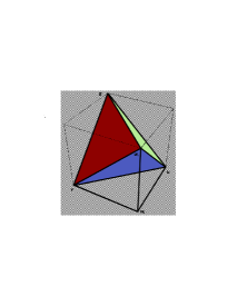
Figure 4.1. Gluing a tetrahedron on the face $\left({\color[rgb]{1,0,0}r},w_{1},{\color[rgb]{0,0,1}b}\right)$

Furthermore the product

$$\left[\mbox{Prod}\left(\mathbf{A},\mbox{Prod}\left(\mathbf{A},\,\mathbf{A},\,\mathbf{A}\right),\mathbf{A}\right)\right]_{{\color[rgb]{1,0,0}r},{\color[rgb]{0,1,0}g},{\color[rgb]{0,0,1}b}}=\sum_{w_{1}}a_{{\color[rgb]{1,0,0}r},w_{1},{\color[rgb]{0,0,1}b}}\,\left(\sum_{w_{0}}a_{{\color[rgb]{1,0,0}r},w_{0},w_{1}}\,a_{{\color[rgb]{1,0,0}r},{\color[rgb]{0,1,0}g},w_{0}}\,a_{w_{0},{\color[rgb]{0,1,0}g},w_{1}}\right)\,a_{w_{1},{\color[rgb]{0,1,0}g},{\color[rgb]{0,0,1}b}}$$

counts the number of tetrahedral simplicial complex which can be constructed by gluing two tetrahedrons at a face of whose labels are of the form $\left({\color[rgb]{1,0,0}r},{\color[rgb]{0,1,0}g},w_{1}\right)$ as depicted in figure 4.2 where the face $\left({\color[rgb]{1,0,0}r},{\color[rgb]{0,1,0}g},w_{1}\right)$ is colored red.

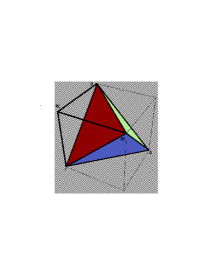
Figure 4.2. Gluing a tetrahedron on the face $\left({\color[rgb]{1,0,0}r},{\color[rgb]{0,1,0}g},w_{1}\right)$

Finally the product

$$\left[\mbox{Prod}\left(\mathbf{A},\mathbf{A},\mbox{Prod}\left(\mathbf{A},\,\mathbf{A},\,\mathbf{A}\right)\right)\right]_{{\color[rgb]{1,0,0}r},{\color[rgb]{0,1,0}g},{\color[rgb]{0,0,1}b}}=\sum_{w_{1}}a_{{\color[rgb]{1,0,0}r},w_{1},{\color[rgb]{0,0,1}b}}\,a_{{\color[rgb]{1,0,0}r},{\color[rgb]{0,1,0}g},w_{1}}\,\left(\sum_{w_{0}}a_{w_{1},w_{0},{\color[rgb]{0,0,1}b}}\,a_{w_{1},{\color[rgb]{0,1,0}g},w_{0}}\,a_{w_{0},{\color[rgb]{0,1,0}g},{\color[rgb]{0,0,1}b}}\right)$$

counts the number of tetrahedral simplicial complex which can be constructed by gluing two tetrahedrons at a face whose labels are of the form $\left(w_{1},{\color[rgb]{0,1,0}g},{\color[rgb]{0,0,1}b}\right)$ as depicted in figure 4.3 where the face $\left(w_{1},{\color[rgb]{0,1,0}g},{\color[rgb]{0,0,1}b}\right)$ is colored green.

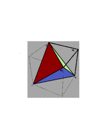
Figure 4.3. Gluing a tetrahedron on the face $\left(w_{1},{\color[rgb]{0,1,0}g},{\color[rgb]{0,0,1}b}\right)$

5. Graph invariants via inflation.

We shall aim to show here that the natural inflation scheme from graph to hypergraphs introduced in [AFW] combined with the combinatorial invariants deduced from the generalization of the Cayley-Hamilton theorem leads to symmetry breaking for some infinite families of cospectral graphs. It is well known that the cospectrality for a pair of graphs $G_{1}$ an $G_{2}$ is equivalent to the assertion that there exist coefficients $\left\{\alpha_{k}\right\}_{0<k\leq n}$ such that

$$\sum_{0<k\leq n+1}\alpha_{k}\;\left(\#\mbox{ Walks of length }k\mbox{ connecting vertex }i\mbox{ to }j\mbox{ in }G_{1}\right)$$

$$=$$

$$\sum_{0<k\leq n+1}\alpha_{k}\;\left(\#\mbox{ Walks of length }k\mbox{ connecting vertex }i\mbox{ to }j\mbox{ in }G_{2}\right)$$

where $\alpha_{n+1}=1$, which algebraically expressed by the following equality in terms of the adjacency matrices

$$\left(\sum_{0<k\leq n+1}\alpha_{k}\,\mathbf{B}^{k}\right)=0=\left(\sum_{0<k\leq n+1}\alpha_{k}\,\mathbf{A}^{k}\right)$$ (5.1)

Incidentally the property can be equivalently stated for an arbitrary sequence of consecutive integer powers of $\mathbf{A}$, namely for some arbitrary integer $\tau\geq 0$

$$\left(\sum_{0<k\leq n+1}\alpha_{k}\,\mathbf{B}^{\tau+k}\right)=0=\left(\sum_{0<k\leq n+1}\alpha_{k}\,\mathbf{A}^{\tau+k}\right)$$ (5.2)

This fact follows from the fact the vector space of powers of a matrix has a span of dimension at most $n$ therefore we can more generally state the cospectral invariance property by stating that

$$0=\sum_{0<k\leq n+1}\left(\#\mbox{ Walks of length }\tau+k\mbox{ connecting }\left(i,j\right)\mbox{ in }G_{1}\right)\alpha_{k}$$

$$=$$

$$\sum_{0<k\leq n+1}\left(\#\mbox{ Walks of length }\tau+k\mbox{ connecting }\left(i,j\right)\mbox{ in }G_{2}\right)\alpha_{k}$$

Theorem 4.

The sequence of sequence of Cayley–Hamilton coefficient are invariant under permutation of hypergaph vertices.

The general argument of the proof is well illustrated for hypermatrices of order $2$ and $4$ it will be immediately apparent how to extend the argument to arbitrary even order hypermartices.

Proof.

The proof that of invariance follows from the fact that the each BM product corresponds to a sum over all vertices. ∎

TheoremTheorem 4 establishes the Cayley–Hamilton coefficient as invariants hypermatrices. Similarly for hypermatrices we may consider the equivalence classes between 3-uniform hypergraphs induced by the

$$0=\sum_{0<k\leq n^{3}+1}\alpha_{k}\>\left(\#\>k\mbox{\textendash Tetrahedral complex spanning }\left({\color[rgb]{1,0,0}u},{\color[rgb]{0,1,0}v},{\color[rgb]{0,0,1}w}\right)\mbox{ in }H_{1}\right)$$

$$=$$

$$\sum_{0<k\leq n^{3}+1}\alpha_{k}\>\left(\#\>k\mbox{\textendash Tetrahedral complex spanning }\left({\color[rgb]{1,0,0}u},{\color[rgb]{0,1,0}v},{\color[rgb]{0,0,1}w}\right)\mbox{ in }H_{2}\right)$$

(where a $k$-Tetrahrdral Simplex denotes a simplex using $k$ vertices in addition to the boundary triangle vertices). The coefficient set $\left\{\alpha_{k}\right\}_{0<k\leq n^{3}+1}$ where $\alpha_{n^{3}+1}=1$, constitutes an invariant for hyperagraph under permutation the vertices of the hypergraph. To show that such invariant are stronger then the spectral invariant it suffices to consider the pair of adjacency matrices with the smallest number of vertices which have the properties that their adjacency matrices are cospectral. A tripartite 3-uniform hypergraph is deduced from a graph as follows. We associate with to every directed path of length two of the form ${\color[rgb]{1,0,0}v_{r}}\rightarrow{\color[rgb]{0,1,0}v_{g}}\rightarrow{\color[rgb]{0,0,1}v_{b}}$, an ordered hyperedge $\left(\mbox{R}_{{\color[rgb]{1,0,0}r}},\mbox{G}_{{\color[rgb]{0,1,0}g}},\mbox{B}_{{\color[rgb]{0,0,1}b}}\right)$ of a hypergraph, thereby setting the $a_{rgb}$ entry of the adjacency hypermatrix to $1$. We refer to such a construction as path adjacency hypermatrix inflation. An easy rank argument on the compositions of products reveals that the inflation scheme in conjunction with the tetrahedral simplex counts indeed distinguishes the original two input isospectral graphs and incidentally establishes the existence of an infinite family of graphs for which the proposed inflation scheme distinguishes isospectral non-isomorphic graphs.

Department of Mathematics, Purdue University
150 N. University Street, West Lafayette, IN 47907-2067
E-mail: egnang@math.purdue.edu

References

- [GER11] E. K. Gnang, A. Elgammal, and V. Retakh, A spectral theory for tensors, Annales de la faculte des sciences de Toulouse Mathematiques 20 (2011), no. 4, 801–841.
- [Gna14] E. K. Gnang, Approximating the spectrum of matrices and hypermatrices, ArXiv e-prints (2014).
- [IGZ94] M.M. Kapranov I.M. Gelfand and A.V. Zelevinsky, Discriminants, resultants and multidimensional determinant, Birkhauser, Boston, 1994.
- [Ker08] Richard Kerner, Ternary and non-associative structures, International Journal of Geometric Methods in Modern Physics 5 (2008), 1265–1294.
- [Lim13] Lek-Heng Lim, Tensors and hypermatrices, Handbook of Linear Algebra (Leslie Hogben, ed.), CRC Press, 2013.
- [Lin11] C-H Lin, Some combinatorial interpretations and applications of fuss-catalan numbers, Discrete Mathematics 2011 (2011).
- [MB90] D. M. Mesner and P. Bhattacharya, Association schemes on triples and a ternary algebra, Journal of combinatorial theory A55 (1990), 204–234.
- [MB94] D. M. Mesner and P. Bhattacharya, A ternary algebra arising from association schemes on triples, Journal of algebra 164 (1994), 595–613.
- [PWZ96] Marko Petkovšek, Herbert S. Wilf, and Doron Zeilberger, A=b, A.K. Peters, 1996.
- [RD08] A. Brualdi Richard and Cvetkovic Dragos, A combinatorial approach to matrix theory and its applications, Chapman and Hall/CRC, 2008.
- [Zei85] Doron Zeilberger, A combinatorial approach to matrix algebra, Discrete Mathematics 56 (1985), 61–72.