Nonequilibrium self-energies, Ng approach and heat current of a nanodevice for small bias voltage and temperature

Abstract

Using non-equilibrium renormalized perturbation theory to second order in the renormalized Coulomb repulsion, we calculate the lesser $\Sigma^{<}$ and and greater $\Sigma^{>}$ self-energies of the impurity Anderson model, which describes the current through a quantum dot, in the general asymmetric case. While in general a numerical integration is required to evaluate the perturbative result, we derive an analytical approximation for small frequency $\omega$, bias voltage $V$ and temperature $T$ which is exact to total second order in these quantities. The approximation is valid when the corresponding energies $\hbar\omega$, $eV$ and $k_{B}T$ are small compared to $k_{B}T_{K}$, where $T_{K}$ is the Kondo temperature. The result of the numerical integration is compared with the analytical one and with Ng approximation, in which $\Sigma^{<}$ and $\Sigma^{>}$ are assumed proportional to the retarded self-energy $\Sigma^{r}$ times an average Fermi function. While it fails at $T=0$ for $\hbar|\omega|\lesssim eV$ we find that the Ng approximation is excellent for $k_{B}T>eV/2$ and improves for asymmetric coupling to the leads. Even at $T=0$, the effect of the Ng approximation on the total occupation at the dot is very small. The dependence on $\omega$ and $V$ are discussed in comparison with a Ward identity that is fulfilled by the three approaches. We also calculate the heat currents between the dot and any of the leads at finite bias voltage. One of the heat currents changes sign with the applied bias voltage at finite temperature.

I Introduction

Progress in nanotechnology has led to the confinement of electrons into small regions, where the electron-electron interactions become increasingly important. Therefore, the interpretation of transport experiments at finite bias voltage $V$, for example different variants of the Kondo effect in transport through quantum dots (QDs),gold ; cro ; wiel ; grobis ; parks ; serge ; ama ; keller requires the theoretical treatment of the effects of both, nonequilibrium physics and strong correlations. This problem is very hard and at present only approximate treatments are used which have different limitations.none ; hbo ; rosch

For nonequilibrium problems, perturbation theory is performed on the Keldysh contour, in which the time evolves from $t_{0}\rightarrow-\infty$ in which the system is in a well defined state and the perturbation is absent, to $t\rightarrow+\infty$ in one branch and returns to the initial state at $t_{0}$ on the other branch of the contour. Thus, the position in the contour is not only given by the time, but also by a branch index. See for example Ref. lif, from which we borrow the notation. As a consequence, there are four different one-particle Green functions depending on the branch index of the creation and annihilation operators. They can be classified  as retarded, advanced, lesser and greater ($G^{r}$, $G^{a}$, $G^{<}$ and $G^{>}$ respectively). Similarly, the Dyson equation leads to four self-energies $\Sigma^{r}$, $\Sigma^{a}$, $\Sigma^{<}$ and $\Sigma^{>}$.none ; lif

In general, it is more difficult to approximate the lesser and greater quantities than the retarded ones. Ng proposed an approximation in which the lesser and greater self-energies $\Sigma^{<}$ and $\Sigma^{>}$ are proportional to average distribution functions ($\tilde{f}(\omega)$ and $\tilde{f}(\omega)-1$ respectively, see Section IV) with the same proportionality factor.ng A consistency equation [Eq. (11)] imposes that this factor is the imaginary part of the retarded self-energy $\Sigma^{r}$. Therefore, this approximation permits to reduce the problem to the calculation of retarded quantities only. The Ng approximation has been used in many different subjects, like Andreev tunneling through strongly interacting QDs,faz spin polarized transport,pz ; ser ; zz first principles calculations of correlated transport through nanojunctions,fer thermopower, dong decoherence effects rap and scaling bal in transport through QDs, magnetotransport in graphene,ding asymmetric effects of the magnetic field in an Aharonov-Bohm interferometer,lim and shot noise in QDs irradiated with microwave fields.zhao Therefore, it is of interest to test this approximation and establish its range of validity. In a recent Letter,mun is was claimed that Ng approximation (Section IV) is exact at low energies. In a Comment to this work we have argued that it is not the case.com In their Reply,reply the authors claim that our analytical result for $\Sigma^{<}$ for zero temperature derived previously does not satisfy a Ward identity, but a direct calculation shows that it does.rr ; note2 This will be shown for all temperatures in Section III.1.2.

One of the approaches used to study the impurity Anderson model (IAM) out of equilibrium is Keldysh perturbation theory in the Coulomb repulsion $U$.none ; hersh ; levy ; fuji ; hama However, it is restricted to small values of $U$. Instead, in renormalized perturbation theory (RPT),he1 the renormalized repulsion $\widetilde{U}$ is always small allowing for a perturbation expansion even if $U\rightarrow\infty$. A calculation of $\Sigma^{r}$ to second order in $\widetilde{U}$ leads to the exact result to total second order in frequency $\omega$, bias voltage $V$ and temperature $T$ in terms of thermodynamic quantities, or the renormalized parameters which can be obtained from exact Bethe ansatz ogu2 or numerical-renormalization-group (NRG) re1 ; re2 calculations at equilibrium. This $\Sigma^{r}$ has been used to obtain the exact form of the conductance through a quantum dot to total second order in $V$ and $T$ for the electron-hole symmetric (EHS) IAM with symmetric voltage drops and coupling to the leads.ogu2 These results are valid for $eV$ and $k_{B}T$ small compared to $k_{B}T_{K}$, where $T_{K}$ is the Kondo temperature. Motivated by recent experiments searching for universal scaling relations for the conductance,grobis ; scott , further developments were made,bal ; rinc ; sela ; roura ; scali but concentrated mainly on the EHS case.

Besides, thermal properties of quantum dots have been studied before,dong ; boese ; kim ; vel ; ss ; see but concentrated mainly on the linear response regime of vanishing voltage and temperature gradient.

In this work we calculate the lesser and greater self-energies of the IAM in the general (not EHS) case, for different (symmetric and asymmetric) coupling to the leads, using RPT to second order in $\widetilde{U}$. The result is compared with the Ng approximation for different temperatures. We derive an exact analytical expression for small $\omega$, $V$ and $T$ (to total second order), useful when the corresponding energies $\hbar\omega$, $eV$ and $k_{B}T$ are small compared to $k_{B}T_{K}$. We also calculate the heat currents between the dot and any of the leads at finite bias voltage and the same temperature for both leads. At $T=0$, an exact analytical expression is provided to third order in $eV/(k_{B}T_{K})$. For finite temperature, a non monotonic behavior of one of the currents is obtained as a function of $V$.

The paper is organized as follows. In Section II we describe the system and the IAM used to represent it. In Section III we review briefly the formalism of the RPT and obtain the analytical expressions for $\Sigma^{<}$ and $\Sigma^{>}$ for small energies. In Section IV we describe the Ng approximation. Section V contains a discussion on the conservation of the current. In Section VI the results for $\Sigma^{<}(\omega)$ calculated with RPT to second order in the renormalized Coulomb repulsion are compared with the Ng approximation and the analytical expression at different voltages and temperatures. In Section VII we show how the bias voltage originate heat currents. Section VIII contains a summary and discussion.

II Model

We use the IAM, to describe a semiconductor QD or a single molecule attached to two conducting leads, with a bias voltage $V$ applied between these leads. The Hamiltonian can be split into a noninteracting part $H_{0}$ and a perturbation $H^{\prime}$ as none ; lady

$$H = H_{0}+H^{\prime},$$

$$H_{0} = \sum_{k\nu\sigma}\varepsilon_{k\nu}\,c_{k\nu\sigma}^{\dagger}c_{k\nu\sigma}+\sum_{\sigma}\varepsilon_{\text{eff}}^{\sigma}\,n_{d\sigma}$$

$$+\sum_{k\nu\sigma}\left(V_{k\nu}\,c_{k\nu\sigma}^{\dagger}d_{\sigma}+\text{H.c.}\right),$$

$$H^{\prime} = \sum_{\sigma}\left(E_{d}-\sigma\mu_{B}B-\varepsilon_{\text{eff}}^{\sigma}\right)\,n_{d\sigma}+U\,n_{d\uparrow}n_{d\downarrow},$$ (1)

where $n_{d\sigma}=d_{\sigma}^{\dagger}d_{\sigma}$, and $\nu=L,R$ refers to the left and right leads. In general $\varepsilon_{\text{eff}}^{\sigma}$ is determined selfconsistently, except for the electron-hole symmetric (EHS) case ($E_{d}=\mu-U/2$) with magnetic field $B=0$, for which $\varepsilon_{\text{eff}}^{\sigma}=\mu$,none ; levy where $\mu$ is the Fermi level which we set as zero in the following.

We write the chemical potentials of both leads in the form

$$\mu_{L}=\alpha_{L}eV\text{, }\mu_{R}=-\alpha_{R}eV,$$ (2)

where $\alpha_{L}+\alpha_{R}=1$. Similarly, the couplings to the leads assumed independent of frequency are expressed in terms of the total resonant level width $\Delta=\Delta_{L}+\Delta_{R}$ as (we take $\hbar=1$ in what follows)

$$\Delta_{\nu}=\pi\sum_{k}|V_{k\nu}|^{2}\delta(\omega-\varepsilon_{k\nu})=\beta_{\nu}\Delta.$$ (3)

III Renormalized perturbation theory

The basic idea of RPT is to reorganize the perturbation expansion in terms of fully dressed quasiparticles in a Fermi liquid picture.he1 The parameters of the original model are renormalized and their values can be calculated exactly from Bethe ansatz results, or accurately using NRG. One of the main advantages is that the renormalized expansion parameter $\widetilde{U}/(\pi\widetilde{\Delta})$ is small. In the EHS case $\widetilde{U}/(\pi\widetilde{\Delta})\leq 1$, being 1 in the extreme Kondo regime ($U=-2E_{d}\rightarrow\infty$).he1 ; ogu2 Within RPT, the low frequency part of $G_{d\sigma}^{r}(\omega)$ is approximated as he1

$$G_{d\sigma}^{r}(\omega)\simeq\frac{z}{\omega-\widetilde{\varepsilon}_{\text{eff}}^{\sigma}+i\widetilde{\Delta}-\widetilde{\Sigma}_{\sigma}^{r}(\omega)},$$ (4)

where $\widetilde{\Delta}=z\Delta$ is the renormalized resonant level width, $z$ is the quasiparticle weight, $\widetilde{\varepsilon}_{\text{eff}}^{\sigma}$ is the renormalized level energy and $\widetilde{\Sigma}_{\sigma}^{r}(\omega)$ is the renormalized retarded self-energy (with $\widetilde{\Sigma}_{\sigma}^{r}(0)=\partial\widetilde{\Sigma}_{\sigma}^{r}(\omega)/\partial\omega=0$ at $V=\omega=0$). $\widetilde{\Delta}$ is of the order of $k_{B}T_{K}$, where $T_{K}$ is the Kondo temperature.

The spectral density of $d$ electrons is $\rho_{\sigma}(\omega)=-\text{Im}G_{d\sigma}^{r}(\omega)/\pi$. The free quasiparticle spectral density of $d$ electrons is given by

$$\widetilde{\rho}_{0}^{\sigma}(\omega)=\frac{\widetilde{\Delta}/\pi}{(\omega-\widetilde{\varepsilon}_{\text{eff}}^{\sigma})^{2}+\widetilde{\Delta}^{2}}.$$ (5)

Both densities at the Fermi energy can be related to the occupancy by the Friedel sum rule lady ; lan

$$\pi\Delta\rho_{\sigma}(0)=\pi\widetilde{\Delta}\widetilde{\rho}^{\sigma}_{0}(0)=\sin^{2}(\pi\langle n_{d\sigma}\rangle),$$ (6)

which allows one to relate the effective dot level with its occupancy

$$\widetilde{\varepsilon}_{\text{eff}}^{\sigma}=\widetilde{\Delta}\cot(\pi\langle n_{d\sigma}\rangle).$$ (7)

The lesser Green’s function can be written in the form none ; scali

$$G_{d\sigma}^{<}(\omega)=\frac{|G_{d\sigma}^{r}(\omega)|^{2}}{z}\left(2i\widetilde{\Delta}\tilde{f}(\omega)-\widetilde{\Sigma}_{\sigma}^{<}(\omega)\right),$$ (8)

where

$$\tilde{f}(\omega)=\sum_{\nu}\beta_{\nu}f(\omega-\mu_{\nu})$$ (9)

is a weighted average of the Fermi functions $f(\omega)=1/(e^{\omega/k_{B}T}+1)$ at the two leads, and $\widetilde{\Sigma}_{\sigma}^{<}(\omega)$ is the renormalized lesser self-energy.

The greater quantities can be obtained from the retarded and lesser ones using the relations lif

$$G^{<}-G^{>}=G^{a}-G^{r}=-2i\text{Im}G^{r}(\omega),$$ (10)

$$\Sigma^{<}-\Sigma^{>}=\Sigma^{a}-\Sigma^{r}=2i\text{Im}\Sigma^{r}(\omega),$$ (11)

where we have used that in the frequency domain, the advanced quantities $G^{a}(\omega)$, $\Sigma^{a}(\omega)$ are the complex conjugates of the corresponding retarded ones.

In the following, we assume that $B=0$ and the leads are paramagnetic, so that the subscript $\sigma$ can be dropped, and $\langle n_{d\sigma}\rangle=n/2$, where $n$ is the total occupancy at the QD.

The linear term in the specific heat and the impurity contribution to the magnetic susceptibility at zero temperature are given by he1

$$\gamma_{C} =2\pi^{2}k_{B}^{2}\widetilde{\rho}_{0}(0)/3,$$ (12)

$$\chi =(g\mu_{B})^{2}\widetilde{\rho}_{0}(0)(1+\widetilde{U}\widetilde{\rho}_{0}(0))/2,$$ (13)

These equations can be inverted to obtain the effective parameters from an accurate knowledge of thermodynamic quantities. For example from Eqs. (6), (7) and (12)

$$\widetilde{\Delta}=\frac{2\pi k_{B}^{2}}{3\gamma_{C}}\sin^{2}(\pi n/2),$$ (14)

and the renormalized interaction is obtained through the Wilson ratio

$$R=\frac{\chi}{\gamma_{C}}\frac{1}{3}\left(\frac{2\pi k_{B}}{g\mu_{B}}\right)^{2}=1+\widetilde{U}\widetilde{\rho}_{0}(0)$$ (15)

III.1 Renormalized lesser and greater self-energies

The renormalized self-energies are calculated as in ordinary perturbation theory in the Keldysh formalism using the low-energy approximation for the unperturbed Green functions.he1 ; ogu1 ; ogu2 To order $\widetilde{U}^{2}$, the renormalized lesser and greater self-energies can be written as none

$$\widetilde{\Sigma}^{<}(\omega) = z\Sigma^{<}(\omega)$$ (16)

$$= -2\pi i\widetilde{U}^{2}\int d\epsilon_{1}d\epsilon_{2}\widetilde{\rho}_{0}(\epsilon_{1})\widetilde{\rho}_{0}(\epsilon_{2})\widetilde{\rho}_{0}(\epsilon_{1}+\epsilon_{2}-\omega)$$

$$\times\tilde{f}(\epsilon_{1})\tilde{f}(\epsilon_{2})(1-\tilde{f}(\epsilon_{1}+\epsilon_{2}-\omega)),$$

$$\widetilde{\Sigma}^{>}(\omega) = 2\pi i\widetilde{U}^{2}\int d\epsilon_{1}d\epsilon_{2}\widetilde{\rho}_{0}(\epsilon_{1})\widetilde{\rho}_{0}(\epsilon_{2})\widetilde{\rho}_{0}(\epsilon_{1}+\epsilon_{2}-\omega)$$ (17)

$$\times(1-\tilde{f}(\epsilon_{1}))(1-\tilde{f}(\epsilon_{2}))\tilde{f}(\epsilon_{1}+\epsilon_{2}-\omega).$$

III.1.1 Analytical approximation for small energies

In this Section we calculate the lesser and greater self-energies assuming that the energies $\omega$, $eV$ and $k_{B}T$ are small in comparison with $\widetilde{\Delta}$, which in turn is of the order of $k_{B}T_{K}$.he1 Specifically, to evaluate the self-energies to total second order in $\omega$, $V$ and $T$, it suffices to replace the quasiparticle spectral density $\widetilde{\rho}_{0}(\epsilon)$ by its value at the Fermi energy (order 0 in an expansion in $\omega$), because the two integrations in Eqs. (16) and (17) already introduce terms of second order, due to the effect of the Fermi functions in restricting the intervals of $\epsilon_{i}$ for which the integrand has non negligible values. For the same reason, terms of higher order in $\widetilde{U}$ lead to terms of higher order in $\omega$, $V$ or $T$. Therefore, the result below is exact to second order. Note that besides the evaluation to second order in $\widetilde{U}$, the only additional approximation is neglecting the energy dependence of $\widetilde{\rho}_{0}(\epsilon)$. The Fermi functions are treated exactly and are not expanded.note2

Using Eq. (9) one sees that

$$\tilde{f}(x)+\tilde{f}(-x)=f(x)+f(-x)=1,$$ (18)

which together with Eq. (9) allows to write the approximation of Eq. (16) for small arguments as

$$\widetilde{\Sigma}_{2}^{<}(\omega,V,T) = -2ip\sum_{\nu\xi\kappa}\beta_{\nu}\beta_{\xi}\beta_{\kappa}\int d\epsilon_{1}d\epsilon_{2}f(\epsilon_{1}-\mu_{\nu})$$ (19)

$$\times f(\epsilon_{2}-\mu_{\xi})f(\omega+\mu_{\kappa}-\epsilon_{1}-\epsilon_{2}),$$

where the factor

$$p = \pi[\widetilde{\rho}_{0}(0)]^{3}\widetilde{U}^{2}=\frac{(R-1)^{2}\sin^{2}(\pi n/2)}{\widetilde{\Delta}}$$ (20)

$$= \frac{3(R-1)^{2}\gamma_{C}}{2\pi k_{B}^{2}}=\frac{2\pi(R-1)^{2}\chi}{R(g\mu_{B})^{2}},$$

can be expressed in terms of the linear term in the specific heat and the magnetic susceptibility at $T=0$.

The integrals in Eq. (19) are evaluated analytically as described in the appendix. The result can be written in the form

$$\widetilde{\Sigma}_{2}^{<} = -ip\sum_{j}c_{j}f(a_{j})\left[a_{j}^{2}+(\pi k_{B}T)^{2}\right],$$

$$c_{1} = \beta_{L}^{2}\beta_{R},\text{ }a_{1}=\omega-(1+\alpha_{L})eV,$$

$$c_{2} = \beta_{L}^{3}+2\beta_{L}\beta_{R}^{2},\text{ }a_{2}=\omega-\alpha_{L}eV,$$

$$c_{3} = \beta_{R}^{3}+2\beta_{L}^{2}\beta_{R},\text{ }a_{3}=\omega+\alpha_{R}eV,$$

$$c_{4} = \beta_{L}\beta_{R}^{2},\text{ }a_{4}=\omega+(1+\alpha_{R})eV.$$ (21)

Particular cases of this low-energy expansion were derived before.hersh ; scali Using Eqs. (17), (18), (19) and (9) one sees that to total second order in $\omega$, $V$ and $T$, the greater self-energy becomes simply

$$\widetilde{\Sigma}_{2}^{>}(\omega,V,T)=-\tilde{\Sigma}_{2}^{<}(-\omega,-V,T).$$ (22)

It is interesting to note that to the same order, calculating the imaginary part of $\widetilde{\Sigma}^{r}$ from the difference Eq. (11), using Eqs. (18), (21) and (22), the Fermi functions disappear and collecting the different terms one recovers the very simple result ogu2

$$\text{Im}\widetilde{\Sigma}_{2}^{r} = -\frac{p}{2}[\omega^{2}-2\gamma\omega eV+\delta(eV)^{2}+(\pi k_{B}T)^{2}],$$ (23)

$$\gamma = \alpha_{L}\beta_{L}-\alpha_{R}\beta_{R},$$ (24)

$$\delta = \gamma^{2}+3\beta_{L}\beta_{R}.$$ (25)

III.1.2 Ward identities

The different self-energies should satisfy the Ward identities ogu1 ; ogu2

$${\frac{\partial\tilde{\Sigma}^{\eta}(\omega)}{\partial eV}\vline}_{V=0}=-\gamma\left(\frac{\partial\tilde{\Sigma}^{\eta}(\omega)}{\partial\omega}+\frac{\partial\tilde{\Sigma}^{\eta}(\omega)}{\partial E_{d}}\right),$$ (26)

where the superscript $\eta$ denotes $>$, $<$, $r$ or $a$, and $\gamma$ is given by Eq. (24). These identities come simply from the properties of the Fermi functions $f(\omega-\mu_{\nu})$ and evaluation at $V=0$ renders both of them equal after derivation [see Eqs. (2)]. They are satisfied at any order in perturbation theory.

Direct differentiation of the analytical expression (21) gives

$${\frac{\partial i\tilde{\Sigma}_{2}^{<}(\omega)}{\partial\omega}\vline}_{V=0} = p\frac{\omega}{1+e^{x}}\left(2-\frac{x}{1+e^{-x}}\right),$$

$$x = \frac{\omega}{k_{B}T}$$ (27)

$${\frac{\partial\tilde{\Sigma}_{2}^{<}(\omega)}{\partial eV}\vline}_{V=0} = -\gamma\frac{\partial\tilde{\Sigma}_{2}^{<}(\omega)}{\partial\omega}.$$ (28)

$\partial\tilde{\Sigma}_{2}^{<}/\partial E_{d}$ can be neglected since it only modifies $\widetilde{\rho}_{0}(0)$ and therefore leads to a contribution of higher order. Thus, $\tilde{\Sigma}_{2}^{<}$ satisfies the Ward identity Eq. (26) to linear order in $\omega$ and $\omega x$. These results will be discussed further in Section VI.3. The $T\rightarrow 0$ limit is well defined and the Ward identity is also satisfied by $\tilde{\Sigma}_{2}^{<}(\omega)$ at $T=0$ in spite of the claim in Ref. reply, that it is not the case.rr ; note2

It is trivial to see that $\text{Im}\tilde{\Sigma}_{2}^{r}$ [Eq. (23)] also satisfies Eq. (26) and from Eq. (11), $\tilde{\Sigma}_{2}^{>}$ satisfies the Ward identity too.

IV Ng approximation

The Ng approximation can be written as

$$\widetilde{\Sigma}_{\text{Ng}}^{<}(\omega)=2i\tilde{f}(\omega)\text{Im}\widetilde{\Sigma}^{r}(\omega),$$ (29)

where $\tilde{f}(\omega)$ is defined by Eq. (9). Using Eq. (8) it can be written in the equivalent form

$$G_{\text{Ng}}^{<}(\omega)=-2i\tilde{f}(\omega)\text{Im}G^{r}(\omega),.$$ (30)

Using Eqs. (10) and (11) also the greater quantities become proportional to the retarded ones:

$$\widetilde{\Sigma}_{\text{Ng}}^{>}(\omega) = -2i[1-\tilde{f}(\omega)]\text{Im}\widetilde{\Sigma}^{r}(\omega),$$ (31)

$$G_{\text{Ng}}^{>}(\omega) = 2i[1-\tilde{f}(\omega)]\text{Im}G^{r}(\omega),.$$ (32)

These equations are exact in the non-interacting case ($U=0$) and also at equilibrium ($V=0$).ng In addition using the results of RPT up to $\widetilde{U}^{2}$ for $\widetilde{\Sigma}^{r}(\omega)$, it can be shown that at $T=0$, the perturbative result $\widetilde{\Sigma}^{<}(\omega)$ and the corresponding Ng approximation $\widetilde{\Sigma}_{\text{Ng}}^{<}(\omega)$ coincide for $\omega<$ -$(1+\alpha_{R})eV$ and $\omega>(1+\alpha_{L})eV$. However, if the expression Eq. (23) for $\text{Im}\widetilde{\Sigma}^{r}(\omega)$ at small energies is replaced in Eq. (29), an analytical expression for $\widetilde{\Sigma}_{\text{Ng}}^{<}(\omega)$ is obtained which is obviously different from the exact result for small $\omega$, $V$ and $T$, Eq. (21). The quantitative differences will be discussed in Section VI.

V Conservation of the current

Using the Keldysh formalism,past ; meir the current flowing between the left lead and the dot can be written as

$$I_{L}=\frac{4ie\Delta_{L}}{h}\int d\omega\left[2if(\omega-\mu_{L})\text{Im}G_{d}^{r}(\omega)+G_{d}^{<}(\omega)\right],$$ (33)

while the current flowing between the dot and the right lead is

$$I_{R}=-\frac{4ie\Delta_{R}}{h}\int d\omega\left[2if(\omega-\mu_{R})\text{Im}G_{d}^{r}(\omega)+G_{d}^{<}(\omega)\right].$$ (34)

Conservation of the current requires $I_{L}=I_{R}=I$.

Using Eqs. (4) and (8), the difference can be written in the form

$$I_{L}-I_{R}=-\frac{4e\widetilde{\Delta}}{h}\int d\omega{\vline\frac{G_{d}^{r}(\omega)}{z}\vline}^{2}[2\tilde{f}(\omega)\text{Im}\widetilde{\Sigma}^{r}(\omega)+i\tilde{\Sigma}^{<}(\omega)].$$ (35)

Using Eqs. (21) and (23), it is easy to see that to total third order in $eV/\widetilde{\Delta}$ and $k_{B}T/\widetilde{\Delta}$ this expression vanishes. Thus RPT conserves the current to this order. Instead, if Ng approximation Eq. (29) is used, $I_{L}-I_{R}$ vanishes identically and the current is conserved to all orders.

VI Lesser self-energy to second order in $\widetilde{U}$

In this Section we present results for $\tilde{\Sigma}^{<}(\omega)$ calculated with RPT to second order in $\widetilde{U}$ by numerical integration. The expression used is equivalent to Eq. (16) but we have used a different approach explained in the appendix of Ref. none, , in which one integral is evaluated analytically. This result $\tilde{\Sigma}^{<}(\omega)$ is superior to the analytical one $\tilde{\Sigma}_{2}^{<}(\omega)$ [Eq. (21)] because no additional approximations (constant quasiparticle density) were made. Both coincide to total second order in $\omega$, $V$ and $T$. Therefore the difference is due to higher order terms in $\tilde{\Sigma}^{<}(\omega)$.

For the calculation of the current, we also need the real part of the renormalized retarded self-energy $\tilde{\Sigma}^{r}(\omega)$, which is also calculated as in Ref. none, with the constant and linear terms in $\omega$ for $V=T=0$ subtracted.he1 ; scali

We have chosen a total occupation $n=2\langle n_{d\sigma}\rangle=3/4$ (out of the EHS case). From Eq. (7) this implies $\widetilde{\varepsilon}_{\text{eff}}^{\sigma}=(\sqrt{2}-1)\widetilde{\Delta}$. We have taken $\widetilde{U}/(\pi\widetilde{\Delta})=1$ for simplicity.note This quotient enters as a constant factor $[\widetilde{U}/(\pi\widetilde{\Delta})]^{2}$ in $\tilde{\Sigma}^{<}(\omega)$ but modifies the values of the current discussed below. Preliminary NRG results indicate that for $E_{d}=-2\Delta$ and $U\rightarrow+\infty$, one has $n=3/4$ and renormalized parameters $z=\widetilde{\Delta}/\Delta=0.115$ and $\widetilde{U}/(\pi\widetilde{\Delta})=1.136$.aap

We assume here a symmetric voltage drop $\alpha_{L}=\alpha_{R}=1/2.$This is motivated by the fact that even for molecular quantum dots with high asymmetric coupling to the leads ($\beta_{L}\gg\beta_{R}$ or $\beta_{L}\ll\beta_{R}$), the shape of the diamonds with the regions of high conductivity as a function of bias voltage $V$ and gate voltage $V_{g}$ indicates a rather symmetric voltage drop. Instead, we consider different ratios of $\beta_{L}/\beta_{R}$.

VI.1 Symmetric coupling to the leads

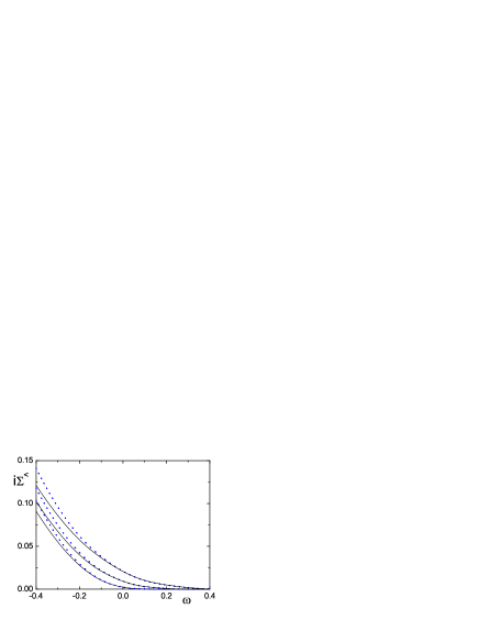
Figure 1: (Color online) Full lines: renormalized lesser self-energy as a function of frequency for $\beta_{L}=\beta_{R}$, $T=0$ and several bias voltages. From bottom to top $eV=$ 0.1, 0.2 and 0.3. Dotted line: analytical result at small energies [Eq. (21)]. $\widetilde{\Delta}=1$ is taken as the unit of energy.

In Fig. 1 we show $\widetilde{\Sigma}^{<}(\omega)$ for $\beta_{L}=\beta_{R}$ and different values of $V$ at zero temperature. In the equilibrium case $V=0$ (not shown), it is known that $\widetilde{\Sigma}^{<}(\omega)=2if(\omega)\text{Im}\widetilde{\Sigma}^{r}(\omega)$, $\widetilde{\Sigma}^{r}(\omega)\sim\omega^{2}$ for small $\omega$ [Eq. (23)] and therefore, $i\widetilde{\Sigma}^{<}(\omega)$ is a decreasing function of $\omega$ for negative $\omega$ and zero for positive $\omega$ at $T=0$. The expression Eq. (21) indicates that the effect of a small voltage is to split this result into four similar expressions, two shifted to smaller $\omega$ and two to higher $\omega.$ The net effect is to increase $i\widetilde{\Sigma}^{<}(\omega)$, but it continues to be a monotonically decreasing function.

The comparison between the numerical result $\widetilde{\Sigma}^{<}(\omega)$ and the analytical one $\widetilde{\Sigma}_{2}^{<}(\omega)$ [Eq. (21)] to total second order in $\omega$ and $V$ is good for $|\omega|<0.2\widetilde{\Delta}$, suggesting that higher order terms are small in this interval. Instead, for $-\omega<0.2\widetilde{\Delta}$, $\widetilde{\Sigma}_{2}^{<}(\omega)$ overestimates $\widetilde{\Sigma}^{<}(\omega)$.

We have also calculated the currents between the left lead and the dot $I_{L}$ and between the dot and the right lead $I_{R}$ for $eV\leq 0.4\widetilde{\Delta}$. The relative error $|I_{L}-I_{R}|/I$, where $I=(I_{L}+I_{R})/2,$ is less than $2.2\times 10^{-4}$ for the values of $eV$ studied. An excellent fit of the difference between currents in this interval is $I_{L}-I_{R}=(2e/h)[-0.00311(eV/\widetilde{\Delta})^{4}-0.00777(eV/\widetilde{\Delta})^{5}]$.note This confirms the analysis of the previous section that the current is conserved to order $V^{3}$ by RPT. In the same interval the current can be fitted by $I=(2e/h)[0.8531(eV/\widetilde{\Delta})-0.1754(eV/\widetilde{\Delta})^{3}]$. The linear term agrees with the expected conductance from Friedel sum rule, proportional to $\sin^{2}(\pi\langle n_{d\sigma}\rangle)=(2+\sqrt{2})/4\approx 0.8536$.

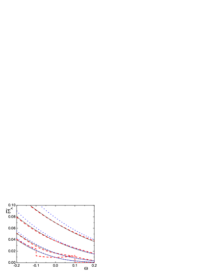
Figure 2: (Color online) Full lines: renormalized lesser self-energy as a function of frequency for $\beta_{L}=\beta_{R}$, $eV=0.2$ and several temperatures. From bottom to top $k_{B}T=$ 0, 0.05, 0.1 and 0.2. Dashed line: Ng approximation [Eq. (29)]. Dotted line: analytical result at small energies [Eq. (21)].

The effect of temperature on $i\widetilde{\Sigma}^{<}(\omega)$ is shown Fig. 2 and the result is compared with the analytical expression for small $\omega$, $V$ and $T$ [Eq. (21)] and the Ng approximation [Eq. (29)]. While as shown above, the former expression $\widetilde{\Sigma}_{2}^{<}(\omega)$ works well at $T=0$, the Ng approximation $\widetilde{\Sigma}_{\text{Ng}}^{<}(\omega)$ fails in the region of small frequencies, below $eV$. In particular, it has jumps at both chemical potentials $\mu_{\nu}$ due to the factor $\tilde{f}(\omega)$ [Eq. (9)] in Eq. (29) and it increases in some interval at positive frequencies in contrast to the overall decreasing behavior of $i\widetilde{\Sigma}^{<}(\omega)$. However, the Ng approximation improves rapidly with increasing temperature. For $k_{B}T=eV/4$, $i\widetilde{\Sigma}_{\text{Ng}}^{<}(\omega)$ lies a little bit below (above) $i\widetilde{\Sigma}^{<}(\omega)$ for $\omega$ near to the smaller (greater) chemical potential. For $k_{B}T=eV/2$, $\widetilde{\Sigma}_{\text{Ng}}^{<}(\omega)$ is already a good approximation for $\widetilde{\Sigma}^{<}(\omega)$ in the whole frequency range. Instead, the analytical expression $\widetilde{\Sigma}_{2}^{<}(\omega)$ overestimates $\widetilde{\Sigma}^{<}(\omega)$ for $k_{B}T\geq eV/2$, particularly at negative frequencies, indicating that terms in temperature of higher order than $T^{2}$ become important.

Concerning the conservation of the current, $|I_{L}-I_{R}|/I$ remains below $0.001$ for $eV=0.2\widetilde{\Delta}$ and $k_{B}T\leq\widetilde{\Delta}$.

VI.2 Larger coupling to the lead of higher chemical potential

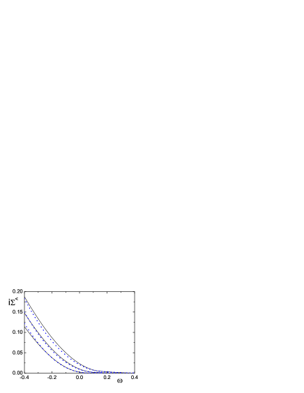
Figure 3: (Color online) Same as Fig. 1 for $\beta_{L}=9\beta_{R}$.

In this Section we study the case $\beta_{L}=9\beta_{R}$. As seen in Fig. 3, increasing the coupling with the left lead, for which the chemical potential $\mu_{L}=\alpha_{L}eV>0$ has the main effect of shifting $i\widetilde{\Sigma}^{<}(\omega)$ to higher frequencies. Since $i\widetilde{\Sigma}^{<}(\omega)$ is a decreasing function of $\omega$, this shift implies higher values $i\widetilde{\Sigma}^{<}(\omega)$ for fixed $\omega$. This can be understood from the analytical expression Eq. (21) in which the terms with coefficients $c_{1}$ and $c_{2}$ increase in magnitude. For $\beta_{L}\rightarrow 1$ ($\beta_{R}\rightarrow 0$), only $c_{2}$ survives and all self-energies reduce to those of a QD at equilibrium with the left lead, $\text{Im}\widetilde{\Sigma}^{r}(\omega)$ behaves as $(\omega-\mu_{L})^{2}$ for small $\omega$ and $V$ at $T=0$ [see Eq. (23)], the Ng approximation becomes exact and $\tilde{f}(\omega)=f(\omega-\mu_{L})$. While this limit is still not reached for $\beta_{L}=9\beta_{R}$, one expects a smaller ratio $|I_{L}-I_{R}|/I$ and a better comparison with the Ng approximation. However, while the currents decrease, the ratio $|I_{L}-I_{R}|/I$ is of the same order of magnitude as before, for the range of voltages studied. The same happens for the case $\beta_{L}=\beta_{R}/9$ discussed in Section VI.3.

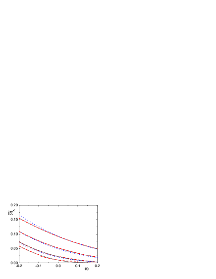
Figure 4: (Color online) Same as Fig. 2 for $\beta_{L}=9\beta_{R}$.

The evolution of $\widetilde{\Sigma}^{<}(\omega)$ with temperature is shown in Fig. 4 and compared with Ng and analytical approximations. At zero temperature, $\widetilde{\Sigma}_{\text{Ng}}^{<}(\omega)$ has qualitatively similar shortcomings as for symmetric coupling to the leads, with jumps at both $\mu_{\nu}$, but quantitatively the agreement is better, as expected. At finite temperature, in this case, already for $k_{B}T=eV/4$, the Ng approximation reproduces very well $\widetilde{\Sigma}^{<}(\omega)$. For higher temperatures the agreement improves, while the analytical approximation $\widetilde{\Sigma}_{2}^{<}$ becomes worse.

VI.3 Larger coupling to the lead of lower chemical potential

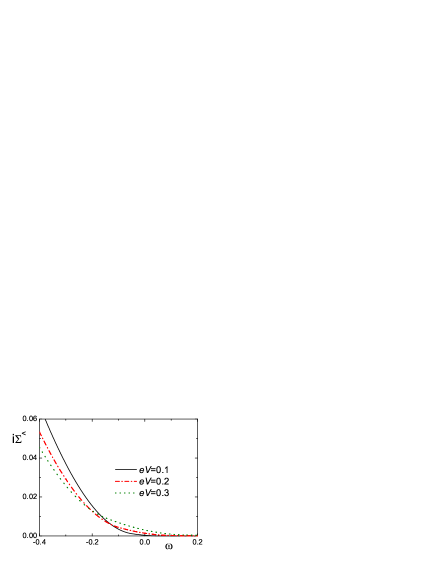
Figure 5: (Color online) Renormalized lesser self-energy as a function of frequency for $\beta_{L}=\beta_{R}/9$, $T=0$ and several bias voltages indicated inside the figure.

In this Section we consider the opposite case as in Section VI.2 and take $\beta_{L}=\beta_{R}/9$. In this case, the system is nearer to the situation in which the dot is at equilibrium with the right lead and similar considerations as in the previous Section apply. In Fig. 5 we display $\widetilde{\Sigma}^{<}(\omega)$ for several values of $V$. While for small $\omega$, $i\widetilde{\Sigma}^{<}(\omega)$ increases with $V$, the behavior changes for $-\omega>eV$ and $i\widetilde{\Sigma}^{<}(\omega)$ decreases with increasing $V$. This can be understood from the Ward identity [Eqs. (28) and (24) for small $\omega$ and $V$]. While the identity is strictly valid for $V=0$ one expects it to be qualitatively valid for small $eV$ compared to $|\omega|$. Since $\partial i\tilde{\Sigma}_{2}^{<}/\partial\omega|_{V=0}$ is negative for negative $\omega$ and also $\gamma$ is negative for large $\beta_{R}$, one expects a decrease of $i\widetilde{\Sigma}^{<}(\omega)$ with increasing $V$ for $eV\ll-\omega$, as observed in Fig. 5.

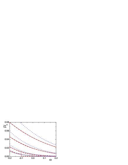
Figure 6: (Color online) Same as Fig. 2 for $\beta_{L}=\beta_{R}/9$.

The effect of temperature on $i\widetilde{\Sigma}^{<}(\omega)$ is shown in Fig. 6. The deviations at zero temperature between the Ng approximation and the correct result to order $\widetilde{U}^{2}$ are larger than in the previous case, particularly for $\omega$ near $\mu_{R}$ ($-0.1\widetilde{\Delta}$ in the figure). However, the comparison improves rapidly with increasing temperature, and $\widetilde{\Sigma}_{\text{Ng}}^{<}(\omega)$ turns out to be a good approximation for $k_{B}T\geq eV/4.$

VII Thermal current induced by the voltage

In this Section, we discuss the heat currents $J_{L}$ flowing from the left lead to the dot and $J_{R}$ flowing from the dot to the right lead. From the thermodynamic equation $dQ=dE-\mu N$, it is clear that

$$J_{\nu}=J_{\nu}^{E}-\mu_{\nu}J_{\nu}^{N},$$ (36)

where $J_{\nu}^{E}$ are the energy currents and $J_{\nu}^{N}$ are the corresponding particle currents.

For a model with nearest-neighbor hopping only, an energy density can be defined and using the continuity equation the energy current can be defined.loza Alternatively, following the definition given by Boese and Fazio boese and using the formalism of Meir and Wingreen,meir one arrives at the same expressions, similar to Eqs. (33) and (34)

$$J_{\nu}^{E}=\pm\frac{4i\Delta_{L}}{h}\int\omega d\omega\left[2if(\omega-\mu_{\nu})\text{Im}G_{d}^{r}(\omega)+G_{d}^{<}(\omega)\right],$$ (37)

where upper (lower) sign corresponds to $\nu=L$ ($R$). These expressions were obtained previously by Dong and Lei,dong who calculated the thermopower of a quantum dot in the linear response regime ($V\rightarrow 0$ and vanishing temperature gradient) using Ng ansatz for $G_{d}^{<}(\omega)$.

The energy current is conserved: $J_{L}^{E}=J_{R}^{E}$. Following a similar reasoning as in Section V, it is easily seen that this condition is satisfied to total fourth order in in $eV/\widetilde{\Delta}$ and $k_{B}T/\widetilde{\Delta}$ by the RPT expressions and exactly by the Ng approximation. Adding the first Eq. (37) for times $\Delta_{L}$ plus the second times $\Delta_{R}$ and using $J_{L}^{E}=J_{R}^{E}$, an expression for the energy current is obtained in which $G_{d}^{<}(\omega)$ is eliminated. The same trick has been used for the electric currents,meir which are the particle currents times the elementary charge: $I_{\nu}=eJ_{\nu}^{N}$. Using this and Eqs. (33) and (34) one obtains

$$J_{\nu}=\frac{8\pi\beta_{L}\beta_{R}\Delta}{h}\int(\omega-\mu_{\nu})d\omega\rho(\omega)[f_{L}(\omega)-f_{R}(\omega)].$$ (38)

Note that the heat current is not conserved. The difference $J_{R}-J_{L}=(\mu_{L}-\mu_{R})I_{v}/e=I_{v}V$ is precisely the Joule heating at the quantum dot.

At zero temperature, the exact heat currents to order $(eV/\widetilde{\Delta})^{3}$ can be obtained using Eq. (6) and scali

$$\frac{\rho(\omega)}{\rho(0)}\simeq 1+\sin(\pi n)\left[\frac{\omega-\gamma(R-1)eV}{\widetilde{\Delta}}\right].$$ (39)

The result is

$$J_{\nu}\simeq\frac{8\beta_{L}\beta_{R}}{h}(eV)^{2}\sin^{2}(\pi n/2)$$ (40)

$$\times \{\frac{\alpha_{L}-\alpha_{R}}{2}+\frac{eV\sin(\pi n)}{\widetilde{\Delta}}[\frac{\alpha_{L}^{3}+\alpha_{R}^{3}}{3}$$

$$-\frac{\gamma(R-1)(\alpha_{L}-\alpha_{R})}{2}]$$

$$\mp \alpha_{\nu}(1+\frac{eV\sin(\pi n)}{\widetilde{\Delta}}[\frac{\alpha_{L}-\alpha_{R}}{2}-\gamma(R-1)])\}.$$

The leading term gives $J_{R}=-J_{L}=G(0)V^{2}/2$, where $G(0)=8\beta_{L}\beta_{R}\sin^{2}(\pi n/2)e^{2}/h$ is the conductance at $V=0$.scali Thus, for small $V$ the heat flow to each lead is the same independently of the particular voltage drops and coupling to the leads.

An analysis of the heat current in the general non-equilibrium case, with different temperatures of the two leads, would require to perform numerically three integrations in frequency. This is highly demanding. Here we study the effect of temperature on the heat current assuming that it is the same for both leads. We have taken $\widetilde{U}/(\pi\widetilde{\Delta})=1.136$. This value was obtained from recent NRG calculations for $E_{d}=-2\Delta$ and $U\rightarrow+\infty$, which also lead to $n=0.75$ and $z=\widetilde{\Delta}/\Delta=0.115$.aap The result for $J_{L}$ for symmetric coupling to the leads and voltage drops $\alpha_{\nu}=\beta_{\nu}=1/2$ is shown in Fig. 7. While for $T=0$, $J_{L}$ is negative, as expected from the leading quadratic term in Eq. (40), the temperature leads to a positive linear term in $V$ (for both heat currents $J_{\nu}$) which dominates the current for small $V$. This positive contribution is expected in linear response, and is consistent with the negative Seebeck coefficient $S$ for temperatures below the Kondo temperature reported previously at equilibrium for $n<1$ ($S$ is proportional to minus the energy current).vel ; see As a consequence, for finite temperatures, $J_{L}$ changes sign as a function of the applied bias voltage. For occupation $n>1$, $S$ is positive and $J_{R}$ changes sign from negative to positive with increasing bias voltage.

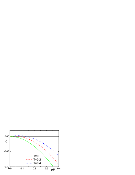
Figure 7: (Color online) Thermal current between the left lead and the quantum dot in units of $\widetilde{\Delta}^{2}/h$ for several temperatures. $\widetilde{\Delta}=1$ is the unit of energy. Parameters in the text.

VIII Summary and discussion

Using renormalized perturbation theory (RPT) to second order in the renormalized Coulomb repulsion $\widetilde{U}$, we have calculated the lesser self-energy $\widetilde{\Sigma}^{<}(\omega)/z$ for the impurity Anderson model, which describes transport through quantum dots, in the general case (without electron-hole symmetry, asymmetric voltage drops and different coupling to the conducting leads). The greater self-energy can be calculated from the difference with the imaginary part of the retarded self-energy [Eq. (11)]. Using an additional approximation, valid for small $\hbar\omega/\widetilde{\Delta}$, $eV/\widetilde{\Delta}$ and $k_{B}T/\widetilde{\Delta}$, where $\widetilde{\Delta}/k_{B}$ is of the order of the Kondo temperature $T_{K}$, we have derived exact analytical expressions to to total second order in $\omega$, $V$ and $T$ for the lesser and greater self-energies. To this end, it is enough to calculate the self-energies to order $\widetilde{U}^{2}$, because higher order terms contribute to higher order in $\omega$, $V$, $T$. The result is given in terms of renormalized parameters, which in turn can be determined directly from NRG re1 ; re2 or from thermodynamic quantities at equilibrium, for which accurate (NRG) bulla or exact (Bethe ansatz) andr ; tsve ; bet ; pedro techniques can be applied.

The resulting $\widetilde{\Sigma}^{<}(\omega)$ (obtained by numerical integration of the diagrammatic expression) is calculated for several values of $V$ and $T$ and different coupling to the leads and compared with the analytical expression and in particular to the Ng approximation [Eq. (29)] widely used in different contexts.pz ; ser ; zz ; fer ; dong ; rap ; bal ; ding ; lim ; zhao While the Ng approximation is inaccurate and presents artificial jumps at $T=0$ for $|\omega|\lesssim eV$, it turns out to be a good approximation in the whole frequency range for $k_{B}T\geq eV/2$ for symmetric coupling to the leads or $k_{B}T\geq eV/4$ for the asymmetric cases studied here.

We have also shown that RPT conserves the current to terms of order $(eV/\widetilde{\Delta})^{3}$ and discussed the dependence of $\widetilde{\Sigma}^{<}(\omega)$ on bias voltage $V$ in terms of Ward identities satisfied by the analytical approximation.

The analytical results for small energies $\hbar\omega$, $eV$ and $k_{B}T$ compared with the quasiparticle level width $\widetilde{\Delta}$ [Eqs. (21) to (23)] can be used to test other approximations for this tough problem, involving strong correlations out of equilibrium.

The RPT approach to order $\widetilde{U}^{2}$ that we have followed becomes invalid for $eV>\widetilde{\Delta}$. In particular, it cannot describe the splitting of the Kondo peak in the spectral density obtained with the non-crossing approximation,win ; nca2 and observed experimentally in a three-terminal quantum ring.letu This might be corrected by the inclusion of terms up to fourth order.fuji

Concerning physical observables, probably the most studied one in the last years is the non-equilibrium electric conductance through nanodevices. In the case of single-level quantum dots for which the impurity Anderson model can be applied, the lesser and greater quantities can be eliminated from the expressions of the conductance using conservation of the current.meir The same happens for the energy current and as a consequence also for the heat current, as shown in Section VII. The lesser (or greater) self-energy plays however a role in this conservation. See Section V. For problems with two levels in which the couplings to both leads are not proportional, such an elimination is not possible and the lesser or greater Green functions enter in the expression for the conductance. An example is the conductance through a benzene molecule connected to the leads in the meta or ortho positions, for which two degenerate levels should be considered (and they couple with different phases to both leads),ben . Other similar systems are molecules with nearly degenerate even and odd states,ball , aromatic molecules or rings of quantum dots,rinc2 or two quantum dots connected with different couplings to two leads.hart In these systems, quantum interference plays an essential role. The case of complete destructive interference is described by an SU(4) Anderson model,interf very similar as the one that describes carbon nanotubes jari ; ander ; buss , silicon nanowires tetta ; see and more recently a double quantum dot with strong interdot capacitive coupling, and each QD tunnel-coupled to its own pair of leads, for certain parameters.ama ; keller ; buss2 ; oks ; nishi The only difference is that the relevant levels are connected to the leads with different phases and therefore the conductance is different. Recently RPT with parameters derived from NRG was applied to this problem for equilibrium quantities. This approach can be extended to study the interference phenomena out of equilibrium.

Another observable, directly related to the lesser Green function is the occupation at the dot, which is given by $\langle n_{d\sigma}\rangle=-i\int d\omega G_{d\sigma}^{<}(\omega)/(2\pi)$.none RPT is not adequate to calculate this integral because it involves energies far from the Fermi level.scali ; he1 However, since the difference between $\widetilde{\Sigma}^{<}(\omega)$ and the corresponding Ng approximation is restricted to energies smaller that $eV$ (see Section IV), we can calculate the effect of this approximation on $n=2\langle n_{d\sigma}\rangle$ using Eq. (8). We find that for the region of parameters that we have studied, the difference $\Delta n=n-n_{\text{Ng}}$ is very small, of the order of $10^{-4}z$. This is due to a large compensation of the regions of positive and negative $\widetilde{\Sigma}_{\text{Ng}}^{>}(\omega)-\widetilde{\Sigma}^{<}(\omega)$. In fact using Eqs. (8), (29) and (35), one realizes that $\Delta n$ is proportional to $I_{L}-I_{R}$ and therefore (from the results of Section V) it is of order $z(eV/\widetilde{\Delta})^{4}$.

Nevertheless, one expects that the shortcomings of the Ng approach would appear in dynamic properties at low frequencies, for which time derivatives enter the conservation laws and the left and right electric and energy currents become different.

We have calculated the effect of the applied bias voltage $V$ on the heat currents between any of the leads and the quantum dot. Due to the joule heating, these currents exits even at zero temperature for $V\neq 0$. We provide exact expressions to order $(eV/\widetilde{\Delta})^{3}$ at $T=0$ [Eq. 40]. At finite temperature, the current between the dot and one of the leads changes sign as a function of $V$.

Appendix A Evaluation of the integrals entering the renormalized lesser self-energy for small energies

The integrals entering Eq. (19) for $\tilde{\Sigma}^{<}(\omega)$ have the form

$$X(\omega) = \int d\epsilon_{2}f(\epsilon_{2}-\mu_{2})Y(\omega,\epsilon_{2}),$$ (41)

$$Y(\omega,\epsilon_{2}) = \int d\epsilon_{1}f(\epsilon_{1}-\mu_{1})f(\omega+\mu_{3}-\epsilon_{1}-\epsilon_{2}).$$ (42)

Using

$$f(x)f(y)=\frac{f(-y)-f(x)}{\exp\left(\frac{x+y}{k_{B}T}\right)-1},$$ (43)

for the integrand of Eq. (42) with $x=\epsilon_{1}-\mu_{1}$, $y=\omega+\mu_{3}-\epsilon_{1}-\epsilon_{2}$, since $\zeta=x+y$ is independent of $\epsilon_{1}$, $Y(\omega,\epsilon_{2})$ becomes proportional to the integral of a difference of Fermi functions. Using

$$\int dx\left[f(x-\zeta)-f(x)\right]=\zeta,$$ (44)

one obtains that $Y(\omega,\epsilon_{2})$ can be written in terms of the Bose function $b(\omega)$

$$Y(\omega,\epsilon_{2}) = \zeta b(\zeta),$$

$$b(\zeta) = \frac{1}{\exp\left(\frac{\zeta}{k_{B}T}\right)-1}$$

$$\zeta = \omega+\mu_{3}-\mu_{1}-\epsilon_{2}.$$ (45)

With the change of variable $v=\epsilon_{2}-\mu_{2}$, replacing Eq. (45) in Eq. (41) one has

$$X(\omega) = \int dv(a-v)f(v)b(a-v),$$

$$a = \omega+\mu_{3}-\mu_{1}-\mu_{2}.$$ (46)

Using

$$f(v)b(a-v)=-f(a)\left[f(v)+b(-a+v)\right],$$ (47)

one can write

$$X(\omega) = f(a)\tilde{X}(\omega),$$ (48)

$$\tilde{X}(\omega) = -\int dv(a-v)\left[f(v)+b(-a+v)\right]$$ (49)

$$= \tilde{X}_{1}(\omega)+\tilde{X}_{2}(\omega),$$

with

$$\tilde{X}_{1}(\omega) = \int dv(v-a)\left[f(v)-f(v-a)\right],$$ (50)

$$\tilde{X}_{2}(\omega) = \int ydy\left[f(y)+b(y)\right]=(k_{B}T)^{2}\int dx\frac{x}{\sinh(x)}$$ (51)

$$= \frac{\pi^{2}}{2}(k_{B}T)^{2}.$$

Above, the changes of variable $y=v-a$, $x=y/(k_{B}T)$ were used.

Using instead $y=v-a/2$, $\tilde{X}_{1}$ becomes

$$\tilde{X}_{1}(\omega) = \int ydy\left[f(y+a/2)-f(y-a/2)\right]$$ (52)

$$-\int dv\left[f(v)-f(v-a)\right]a/2.$$

The first integral vanishes, since the integrand is odd [as can be checked using Eq. (18)]. Using Eq. (44) the second integral gives $\tilde{X}_{1}(\omega)=a^{2}/2$. Replacing this and Eq. (51) in Eq. (48) we finally obtain

$$X(\omega)=\frac{f(a)}{2}\left[a^{2}+(\pi k_{B}T)^{2}\right].$$ (53)

References

- (1) D. Goldhaber-Gordon, H. Shtrikman, D. Mahalu, D. Abusch-Magder, U. Meirav, and M. A. Kastner, Nature 391, 156 (1998).
- (2) S. M. Cronenwet, T. H. Oosterkamp, and L. P. Kouwenhoven, Science 281, 540 (1998).
- (3) W.G. van der Wiel, S. de Franceschi, T. Fujisawa, J.M. Elzerman, S. Tarucha, and L.P. Kowenhoven, Science 289, 2105 (2000).
- (4) M. Grobis, I. G. Rau, R. M. Potok, H. Shtrikman, and D. Goldhaber-Gordon, Phys. Rev. Lett. 100, 246601 (2008).
- (5) J. J. Parks, A. R. Champagne, T. A. Costi, W. W. Shum, A. N. Pasupathy, E. Neuscamman, S. Flores-Torres, P. S. Cornaglia, A. A. Aligia, C. A. Balseiro, G. K.-L. Chan, H. D. Abruña, and D. C. Ralph, Science 328, 1370 (2010)
- (6) S. Florens, A, Freyn, N. Roch, W. Wernsdorfer, F. Balestro, P. Roura-Bas and A. A. Aligia, J. Phys. Condens. Matter 23, 243202 (2011); references therein.
- (7) S. Amasha, A. J. Keller, I. G. Rau, A. Carmi, J. A. Katine, H. Shtrikman, Y. Oreg, and D. Goldhaber-Gordon, Phys. Rev. Lett. 110, 046604 (2013).
- (8) A. J. Keller, S. Amasha, I. Weymann, C. P. Moca, I. G. Rau, J. A. Katine, H. Shtrikman, G. Zaránd, and D. Goldhaber-Gordon, arXiv:1306.6326), Nature Physics doi:10.1038/nphys2844.
- (9) A. A. Aligia, Phys. Rev. B 74, 155125 (2006); references therein.
- (10) A. C. Hewson, J. Bauer, and A, Oguri, J. Phys. Condens. Matter 17, 5413 (2005); references therein.
- (11) A. Rosch, Eur. Phys. J. B 85, 6 (2012).
- (12) E.M. Lifshitz and A.L. Pitaevskii, Physical Kinetics (Pergamon, Oxford, 1981).
- (13) T-K Ng, Phys. Rev. Lett. 76, 487 (1996).
- (14) R. Fazio, and R. Raimondi, Phys. Rev. Lett. 80, 2913 (1998).
- (15) P. Zhang, Q.-K. Xue, Y. P. Wang, and X. C. Xie, Phys. Rev. Lett. 89, 286803 (2002).
- (16) N. Sergueev, Q.-F. Sun, H. Guo, B. G. Wang, and J. Wang, Phys. Rev. B 65, 165303 (2002).
- (17) H. Zhang, G-M. Zhang, and Lu Yu, J. Phys. Condens. Matter 21, 155501 (2009).
- (18) A. Ferretti, A. Calzolari, R. DiFelice, F. Manghi, M. J. Caldas, M. Buongiorno Nardelli, and E. Molinari, Phys. Rev. Lett. 94, 116802 (2005).
- (19) B. Dong and X. L. Lei, J. Phys. Condens. Matter 14, 11747 (2002).
- (20) R. Van Roermund, S. Y. Shiau, and M. Lavagna, Phys. Rev. B 81, 165115 (2010).
- (21) C. A. Balseiro, G. Usaj, and M. J. Sánchez, J. Phys. Condens. Matter 22, 425602 (2010).
- (22) K.-H. Ding, Z.-G. Zhu, Z.-H. Zhang, and J. Berakdar, Phys. Rev. B 82, 155143 (2010).
- (23) J. S. Lim, D. Sánchez, and R. López, Phys. Rev. B 81, 155323 (2010).
- (24) H. K. Zhao and L. L. Zhao, Europhys. Lett. 93, 28004 (2011).
- (25) E. Muñoz, C. J. Bolech, and S. Kirchner, Phys. Rev. Lett. 110, 016601 (2013).
- (26) A. A. Aligia, Phys. Rev. Lett. 111, 089701 (2013).
- (27) E. Muñoz, C. J. Bolech, and S. Kirchner, Phys. Rev. Lett. 111, 089702 (2013).
- (28) A. A. Aligia, arXiv:1310.8324
- (29) The failure of the argument in the reply reply in its claiming that the Ward identity is not satisfied is due to the fact that it is based on an inappropriate expansion of for around the singular point . To illustrate the point, let us consider the function [similar to Eq. (21) at ] , where is the step function. Expanding this function to total second order around the origin gives , which is obviously very different from out of the origin. In particular even for a tiny , . According to Ref. reply, , cannot have a term in for small and because does not have it.
- (30) S. Hershfield, J.H. Davies, and J.W. Wilkins, Phys. Rev. B 46, 7046 (1992).
- (31) A. Levy-Yeyati, A. Martín-Rodero, and F. Flores, Phys. Rev. Lett. 71, 2991 (1993).
- (32) T. Fujii and K. Ueda, Phys. Rev. B 68, 155310 (2003), J. Phys. Soc. Jpn. 74, 127 (2005).
- (33) M. Hamasaki, Condensed Matter Physics 10, 235 (2007).
- (34) A. C. Hewson, Phys. Rev. Lett. 70, 4007 (1993).
- (35) A. Oguri, Phys. Rev. B 64, 153305 (2001).
- (36) A. Oguri, J. Phys. Soc. Jpn. 74, 110 (2005).
- (37) A. C. Hewson, A. Oguri and D. Meyer, Euro. Phys. J. B 40, 177 (2004)
- (38) A. C. Hewson, J. Phys. Soc. Japan, 74, 8 (2005).
- (39) G. D. Scott, Z. K. Keane, J. W. Ciszek, J. M. Tour, and D. Natelson, Phys. Rev. B 79, 165413 (2009).
- (40) J. Rincón, A. A. Aligia, and K. Hallberg, Phys. Rev. B 79, 121301(R) (2009); arXiv:0901.4326.
- (41) E. Sela and J. Malecki, Phys. Rev. B 80, 233103 (2009).
- (42) P. Roura-Bas, Phys. Rev. B 81, 155327 (2010).
- (43) A. A. Aligia, J. Phys. Condens. Matter 24, 015306 (2012).
- (44) D. Boese and R. Fazio, Europhys. Lett. 56, 576 (2001).
- (45) T.-S. Kim and S. Hershfield, Phys. Rev. Lett. 88, 136601 (2002).
- (46) T. A. Costi and V. Zlatić, Phys. Rev. B 81, 235127 (2010).
- (47) P. S. Cornaglia, G. Usaj, and C. A. Balseiro, Phys. Rev. B 86, 041107
- (48) P. Roura-Bas, L. Tosi, A. A. Aligia, and P. S. Cornaglia, Phys. Rev. B 86, 165106 (2012).
- (49) A. A. Aligia and L. A. Salguero, Phys. Rev. B 70, 075307 (2004); Phys. Rev. B 71, 169903(E) (2005).
- (50) D. C. Langreth, Phys. Rev. 150, 516 (1966).
- (51) H. M. Pastawski, Phys. Rev. B 46, 4053 (1992).
- (52) Y. Meir and N. S. Wingreen, Phys. Rev. Lett. 68, 2512 (1992).
- (53) The precise values of the current depend on the exact value of , but this does not modify our conclusions.
- (54) J. A. Andrade, A. A. Aligia and P. S. Cornaglia, in preparation.
- (55) L. Arrachea, G. S. Lozano, and A. A. Aligia, Phys. Rev. B 80, 014425 (2009).
- (56) R. Bulla, T. A. Costi, and T. Pruschke, Rev. Mod. Phys.. 80, 395 (2008).
- (57) N. Andrei, K. Furuya, and J. H. Lowenstein, Rev. Mod. Phys. 55, 331 (1983).
- (58) A. M. Tsvelick and P. B. Wiegmann, Adv. Phys.32, 453 (1983).
- (59) A. A. Aligia, C. A. Balseiro and C. R. Proetto, Phys. Rev. B 33, 6476 (1986).
- (60) P. Schlottmann, Phys. Rep. 181, 1 (1989).
- (61) N.S. Wingreen and Y. Meir, Phys. Rev. B 49, 11040 (1994).
- (62) M. H. Hettler, J. Kroha and S. Hershfield, Phys. Rev. B 58, 5649 (1998).
- (63) R. Leturcq, L. Schmid, K. Ensslin, Y. Meir, D.C. Driscoll, and A.C. Gossard, Phys. Rev. Lett. 95, 126603 (2005).
- (64) L. Tosi, P. Roura-Bas, and A. A. Aligia, J. Phys. Condens. Matter 24, 365301 (2012); references therein.
- (65) S. Ballmann, R. Hãrtle, P. B. Coto, M. Elbing, M. Mayor, M. R. Bryce, M. Thoss, and H. B. Weber, Phys. Rev. Lett. 109, 056801 (2012).
- (66) J. Rincón, K. Hallberg, A. A. Aligia, and S. Ramasesha, Phys. Rev. Lett. 103, 266807 (2009).
- (67) R. Hãrtle, G. Cohen, D. R. Reichman, and A. J. Millis, Phys. Rev. B 88, 235426 (2013).
- (68) P. Roura-Bas, L. Tosi, A. A. Aligia, and K. Hallberg, Phys. Rev. B 84, 073406 (2011).
- (69) P. Jarillo-Herrero, J. Kong, H. S. J. van der Zant, C. Dekker, L. P. Kouwenhoven, and S. De Franceschi, Nature 434, 484 (2005).
- (70) F. B. Anders, D. E. Logan, M. R. Galpin, and G. Finkelstein, Phys. Rev. Lett. 100, 086809 (2008).
- (71) C. A. Büsser, E. Vernek, P. Orellana, G. A. Lara, E. H. Kim, A. E. Feiguin, E. V. Anda, and G. B. Martins, Phys. Rev. B 83, 125404 (2011).
- (72) G. C. Tettamanzi, J. Verduijn, G. P. Lansbergen, M. Blaauboer, M. J. Calderón, R. Aguado, and S. Rogge, Phys. Rev. Lett. 108, 046803 (2012).
- (73) C. A. Büsser, A. E. Feiguin, and G. B. Martins, Phys. Rev. B 85, 241310(R) (2012).
- (74) L. Tosi, P. Roura-Bas, and A. A. Aligia, Phys. Rev. B 88, 235427 (2013).
- (75) Y. Nishikawa, A. C. Hewson, D. J.G. Crow, and J. Bauer, Phys. Rev. B 88, 245130 (2013).