Two-Point $L_{1}$ Shortest Path Queries in the Plane

Abstract

Let $\mathcal{P}$ be a set of $h$ pairwise-disjoint polygonal obstacles with a total of $n$ vertices in the plane. We consider the problem of building a data structure that can quickly compute an $L_{1}$ shortest obstacle-avoiding path between any two query points $s$ and $t$. Previously, a data structure of size $O(n^{2}\log n)$ was constructed in $O(n^{2}\log^{2}n)$ time that answers each two-point query in $O(\log^{2}n+k)$ time, i.e., the shortest path length is reported in $O(\log^{2}n)$ time and an actual path is reported in additional $O(k)$ time, where $k$ is the number of edges of the output path. In this paper, we build a new data structure of size $O(n+h^{2}\cdot\log h\cdot 4^{\sqrt{\log h}})$ in $O(n+h^{2}\cdot\log^{2}h\cdot 4^{\sqrt{\log h}})$ time that answers each query in $O(\log n+k)$ time. Note that $n+h^{2}\cdot\log^{2}h\cdot 4^{\sqrt{\log h}}=O(n+h^{2+\epsilon})$ for any constant $\epsilon>0$. (In contrast, for the Euclidean version of this two-point query problem, the best known algorithm uses $O(n^{11})$ space to achieve an $O(\log n+k)$ query time.) In addition, we construct a data structure of size $O(n+h^{2}\log^{2}h)$ in $O(n+h^{2}\log^{2}h)$ time that answers each query in $O(\log n+\log^{2}h+k)$ time, and a data structure of size $O(nh\log h)$ in $O(nh\log h+h^{2}\log^{2}h)$ time that answers each query in $O(\log n\log h+k)$ time. Further, we extend our techniques to the weighted rectilinear version in which the “obstacles” of $\mathcal{P}$ are rectilinear regions with “weights” and allow $L_{1}$ paths to travel through them with weighted costs. Previously, a data structure of size $O(n^{2}\log^{2}n)$ was built in $O(n^{2}\log^{2}n)$ time that answers each query in $O(\log^{2}n+k)$ time. Our new algorithm answers each query in $O(\log n+k)$ time with a data structure of size $O(n^{2}\cdot\log n\cdot 4^{\sqrt{\log n}})$ that is built in $O(n^{2}\cdot\log^{2}n\cdot 4^{\sqrt{\log n}})$ time (note that $n^{2}\cdot\log^{2}n\cdot 4^{\sqrt{\log n}}=O(n^{2+\epsilon})$ for any constant $\epsilon>0$).

1 Introduction

Let $\mathcal{P}$ be a set of $h$ pairwise-disjoint polygonal obstacles in the plane with a total of $n$ vertices. We consider two-point shortest obstacle-avoiding path queries for which the path lengths are measured in the $L_{1}$ metric. The plane minus the interior of the obstacles is called the free space. Our goal is to build a data structure to quickly compute an $L_{1}$ shortest path in the free space between any two query points $s$ and $t$. Previously, Chen et al. [6] constructed a data structure of size $O(n^{2}\log n)$ in $O(n^{2}\log^{2}n)$ time that computes the length of the $L_{1}$ shortest $s$-$t$ path in $O(\log^{2}n)$ time and an actual path in additional $O(k)$ time, where $k$ is the number of edges of the output path. Throughout this paper, unless otherwise stated, when we say that the query time of a data structure is $O(f(n,h))$ (which may be a function of both $n$ and $h$), we mean that the shortest path length can be reported in $O(f(n,h))$ time and an actual path can be found in additional time linear in the number of edges of the output path. Hence, the query time of the data structure in [6] is $O(\log^{2}n)$.

In this paper, we build a new data structure of size $O(n+h^{2}\cdot\log h\cdot 4^{\sqrt{\log h}})$ in $O(n+h^{2}\cdot\log^{2}h\cdot 4^{\sqrt{\log h}})$ time, with $O(\log n)$ query time. Note that $n+h^{2}\cdot\log^{2}h\cdot 4^{\sqrt{\log h}}=O(n+h^{2+\epsilon})$ for any constant $\epsilon>0$. Hence, comparing with the results in [6], we reduce the query time by a logarithmic factor, and use less preprocessing time and space when $h$ is small, e.g., $h=O(n^{\delta})$ for any constant $\delta<1$. In addition, we can also build a data structure of size $O(n+h^{2}\log^{2}h)$ in $O(n+h^{2}\log^{2}h)$ time, with an $O(\log n+\log^{2}h)$ query time, and another data structure of size $O(nh\log h)$ in $O(nh\log h+h^{2}\log^{2}h)$ time, with an $O(\log n\log h)$ query time.

Further, we extend our techniques to the weighted rectilinear version in which each “obstacle” $P\in\mathcal{P}$ is a region with a nonnegative weight $w(P)$ and the edges of the obstacles in $\mathcal{P}$ are all axis-parallel; a path intersecting the interior of $P$ is charged a cost depending on $w(P)$. For this problem, Chen et al. [6] constructed a data structure of size $O(n^{2}\log^{2}n)$ in $O(n^{2}\log^{2}n)$ time that answers each two-point shortest path query in $O(\log^{2}n)$ time. We build a new data structure of size $O(n^{2}\cdot\log n\cdot 4^{\sqrt{\log n}})$ in $O(n^{2}\cdot\log^{2}n\cdot 4^{\sqrt{\log n}})$ time that answers each query in $O(\log n)$ time. Note that $n^{2}\cdot\log^{2}n\cdot 4^{\sqrt{\log n}}=O(n^{2+\epsilon})$ for any constant $\epsilon>0$.

1.1 Related Work

The problems of computing shortest paths among obstacles in the plane have been studied extensively (e.g., [5, 6, 7, 8, 10, 11, 18, 19, 20, 21, 22, 23, 24, 25, 26, 27, 30, 33, 34, 35, 36, 37, 38]). There are three main types of such problems: finding a single shortest $s$-$t$ path (both $s$ and $t$ are given as part of the input and the goal is to find a single shortest $s$-$t$ path), single-source shortest path queries ($s$ is given as part of the input and the goal is to build a data structure to answer shortest path queries for any query point $t$), and two-point shortest path queries (as defined and considered in this paper). The distance metrics can be the Euclidean (i.e., $L_{2}$) or $L_{1}$. Refer to [39] for a comprehensive survey on this topic.

For the simple polygon case, in which $\mathcal{P}$ is a single simple polygon, all three types of problems have been solved optimally [19, 20, 21, 23, 33], in both the Euclidean and $L_{1}$ metrics. Specifically, an $O(n)$-size data structure can be built in $O(n)$ time that answers each two-point Euclidean shortest path query in $O(\log n)$ time [19, 21]. Since in a simple polygon a Euclidean shortest path is also an $L_{1}$ shortest path [23], the results in [19, 21] hold for the $L_{1}$ metric as well.

The polygonal domain case (or “a polygon with holes”), in which $\mathcal{P}$ has $h$ obstacles as defined above, is more difficult. For the Euclidean metric, Hershberger and Suri [24] built a single source shortest path map of size $O(n\log n)$ in $O(n\log n)$ time that answers each query in $O(\log n)$ time. For the $L_{1}$ metric, Mitchell [35, 37] built an $O(n)$-size single source shortest path map in $O(n\log n)$ time that answers each query in $O(\log n)$ time. Later, Chen and Wang [7, 8, 11] built an $L_{1}$ single source shortest path map of size $O(n)$ in $O(n+h\log h)$ time, with an $O(\log n)$ query time, for a triangulated free space (the current best triangulation algorithm takes $O(n+h\log^{1+\epsilon}h)$ time for any constant $\epsilon>0$ [2]). For two-point $L_{1}$ shortest path queries, Chen et al. [6] gave the previously best solution, as mentioned above; for a special case where the obstacles are rectangles, ElGindy and Mitra [18] gave an $O(n^{2})$ size data structure that supports $O(\log n)$ time queries. For two-point queries in the Euclidean metric, Chiang and Mitchell [14] constructed a data structure of size $O(n^{11})$ that answers each query in $O(\log n)$ time, and alternatively, a data structure of size $O(n^{10}\log n)$ with an $O(\log^{2}n)$ query time; other data structures with trade-off between preprocessing and query time were also given in [14]. If the query points $s$ and $t$ are both restricted to the boundaries of the obstacles of $\mathcal{P}$, Bae and Okamato [1] built a data structure of size $O(n^{5}{\rm poly}(\log n))$ that answers each query in $O(\log n)$ time, where ${\rm poly}(\log n)$ is a polylogarithmic factor. Efficient algorithms were also given for the case when the obstacles have curved boundaries [5, 10, 13, 22, 25].

For the weighted region case, in which the “obstacles” allow paths to pass through their interior with weighted costs, Mitchell and Papadimitriou [40] gave an algorithm that finds a weighted Euclidean shortest path in a time of $O(n^{8})$ times a factor related to the precision of the problem instance. For the weighted rectilinear case, Lee et al. [34] presented two algorithms for finding a weighted $L_{1}$ shortest path, and Chen et al. [6] gave an improved algorithm with $O(n\log^{3/2}n)$ time and $O(n\log n)$ space. Chen et al. [6] also presented a data structure for two-point weighted $L_{1}$ shortest path queries among weighted rectilinear obstacles, as mentioned above.

1.2 Our Approaches

Our first main idea is to propose an enhanced graph model based on the scheme in [6, 15, 16], to reduce the query time from $O(\log^{2}n)$ to $O(\log n)$. In [6, 15, 16], to build a graph, a total of $n$ vertical lines (called “cut-lines”) are created recursively in $O(\log n)$ levels. Then, each obstacle vertex $v$ is projected to $O(\log n)$ cut-lines (one cut-line per level) to create “Steiner points” if $v$ is horizontally visible to such cut-lines. For any two query points $s$ and $t$, to report an $L_{1}$ shortest $s$-$t$ path, the algorithm in [6] finds $O(\log n)$ Steiner points (called “gateways”) on $O(\log n)$ cut-lines for each of $s$ and $t$, such that there must be a shortest $s$-$t$ path containing a gateway of $s$ and a gateway of $t$. Consequently, a shortest path is obtained in $O(\log^{2}n)$ time using the $O(\log n)$ gateways of $s$ and $t$.

We propose an enhanced graph $G_{E}$ by adding more Steiner points onto the cut-lines such that we need only $O(\sqrt{\log n})$ gateways for any query points, and consequently, computing the shortest path length takes $O(\log n)$ time. More specifically, for each obstacle vertex, instead of projecting it to a single vertical cut-line at each level, we project it to $O(2^{\sqrt{\log n}})$ cut-lines in every $O(\sqrt{\log n})$ consecutive levels (thus creating $O(2^{\sqrt{\log n}})$ Steiner points); in fact, these cut-lines form a binary tree structure of height $O(\sqrt{\log n})$ and they are carefully chosen to ensure that $O(\sqrt{\log n})$ gateways are sufficient for any query point. Hence, the size of the graph $G_{E}$ is $O(n\sqrt{\log n}2^{\sqrt{\log n}})$.

To improve the data structure construction so that its time and space bounds depend linearly on $n$, we utilize the extended corridor structure [7, 8, 11], which partitions the free space of $\mathcal{P}$ into an “ocean” $\mathcal{M}$, and multiple “bays” and “canals”. We build a graph $G_{E}(\mathcal{M})$ of size $O(h\sqrt{\log h}2^{\sqrt{\log h}})$ on $\mathcal{M}$ similar to $G_{E}$, such that if both query points are in $\mathcal{M}$, then the query can be answered in $O(\log n)$ time. It remains to deal with the general case when at least one query point is not in $\mathcal{M}$. This is a major difficulty in our problem and our algorithm for this case is another of our main contributions. Below, we use a bay as an example to illustrate our main idea for this algorithm.

For two query points $s$ and $t$, suppose $s$ is in a bay $B$ and $t$ is outside $B$. Since $B$ is a simple polygon, any shortest $s$-$t$ path must cross the “gate” $g$ of $B$, which is a single edge shared by $B$ and $\mathcal{M}$. We prove that there exists a shortest $s$-$t$ path that must contain one of three special points $z(s)$, $z_{1}(s)$, and $z_{2}(s)$, where $z(s)$ is in $B$ and the other two points are on $g$ (and thus in $\mathcal{M}$). For the case when a shortest $s$-$t$ path contains either $z_{1}(s)$ or $z_{2}(s)$, we can use the graph $G_{E}(\mathcal{M})$ to find such a shortest path. For the other case, we build another graph $G_{E}(g)$ based on the horizontal projections of the vertices of $G_{E}(\mathcal{M})$ on $g$, and use $G_{E}(g)$ to find such a shortest path (along with a set of interesting observations) by a merge of $G_{E}(g)$ and $G_{E}(\mathcal{M})$. Intuitively, $G_{E}(g)$ plays the role of connecting the shortest path structure inside $B$ with those in $\mathcal{M}$.

The case when a query point is in a canal can be handled similarly in spirit, although it is more complicated because each canal has two gates.

The rest of the paper is organized as follows. In Section 2, we introduce some notations and sketch the previous results that will be needed by our algorithms. In Section 3, we propose our enhanced graph $G_{E}$ that helps reduce the query time to $O(\log n)$. In Section 4, we further reduce the preprocessing time and space by using the extended corridor structure. In Section 5, we extend our techniques in Section 3 to the weighted rectilinear case.

Henceforth, unless otherwise stated, “shortest paths” always refer to $L_{1}$ shortest paths and “distances” and “lengths” always refer to $L_{1}$ distances and lengths. To distinguish from graphs, the vertices/edges of $\mathcal{P}$ are always referred to as obstacle vertices/edges, and graph vertices are referred to as “nodes”. For simplicity of discussion, we make a general position assumption that no two obstacle vertices have the same $x$- or $y$-coordinate except for the weighted rectilinear case.

2 Preliminaries

A path in the plane is $x$-monotone (resp., $y$-monotone) if its intersection with any vertical (resp., horizontal) line is either empty or connected. A path is $xy$-monotone if it is both $x$-monotone and $y$-monotone. It is well-known that any $xy$-monotone path is an $L_{1}$ shortest path.

A point $p$ is visible to another point $q$ if the line segment $\overline{pq}$ entirely is in the free space. A point $p$ is horizontally visible to a line $l$ if there is a point $q$ on $l$ such that $\overline{pq}$ is horizontal and is in the free space. For a line $l$ and a point $p$, the point $q\in l$ is the horizontal projection of $p$ on $l$ if $\overline{pq}$ is horizontal, and we denote it by $p_{h}(l)=q$. Let $\partial\mathcal{P}$ denote the boundaries of all obstacles in $\mathcal{P}$. For a point $p$ in the free space of $\mathcal{P}$, if we shoot a horizontal ray from $p$ to the left, the first point on $\partial\mathcal{P}$ hit by the ray is called the leftward projection of $p$ on $\partial\mathcal{P}$, denoted by $p^{l}$; similarly, we define the rightward, upward, and downward projections of $p$ on $\partial\mathcal{P}$, denoted by $p^{r}$, $p^{u}$, and $p^{d}$, respectively.

We sketch the graph in [6], denoted by $G_{old}$, for answering two-point queries, which was originally proposed in [15, 16] for computing a single shortest path. To define $G_{old}$, two types of Steiner points are specified, as follows. For each obstacle vertex $p$, its four projections on $\partial\mathcal{P}$, i.e., $p^{l},p^{r},p^{u}$, and $p^{d}$, are type-1 Steiner points. Clearly, there are $O(n)$ type-1 Steiner points in total.

The type-2 Steiner points are on cut-lines. In order to facilitate an explanation on our new graph model in Section 3, we organize the cut-lines in a binary tree structure, called the cut-line tree and denoted by $T(\mathcal{P})$. The tree $T(\mathcal{P})$ is defined as follows. For each node $u$ of $T(\mathcal{P})$, a set $V(u)$ of obstacle vertices and a cut-line $l(u)$ are associated with $u$, where $l(u)$ is a vertical line through the median of the $x$-coordinates of the obstacle vertices in $V(u)$. For the root $r$ of $T(\mathcal{P})$, $V(r)$ is the set of all obstacle vertices of $\mathcal{P}$. For the left (resp., right) child $v$ of $u$, $V(v)$ consists of the obstacle vertices of $V(u)$ on the left (resp., right) of $l(u)$. Since the number of vertices of $\mathcal{P}$ is $n$, the height of $T(\mathcal{P})$ is $O(\log n)$. For every node $u$ of $T(\mathcal{P})$, for each vertex $p\in V(u)$, if $p$ is horizontally visible to $l(u)$, then the point $p_{h}(l(u))$, i.e., the horizontal projection of $p$ on $l(u)$, is a type-2 Steiner point. Since each obstacle vertex defines a type-2 Steiner point on at most one cut-line at each level of $T(\mathcal{P})$, there are $O(n\log n)$ type-2 Steiner points.

The node set of $G_{old}$ consists of all obstacle vertices of $\mathcal{P}$ and all Steiner points thus defined.

The edges of $G_{old}$ are defined as follows. First, for every obstacle vertex $p$, there is an edge $\overline{pq}$ in $G_{old}$ for each $q\in\{p^{l},p^{r},p^{u},p^{d}\}$. Second, for every obstacle edge $e$ of $\mathcal{P}$, $e$ may contain multiple type-1 Steiner points, and these Steiner points and the two endpoints of $e$ are the nodes of $G_{old}$ on $e$; the segment connecting each pair of consecutive graph nodes on $e$ defines an edge in $G_{old}$. Third, for each cut-line $l$, any two consecutive type-2 Steiner points on $l$ define an edge in $G_{old}$ if these two points are visible to each other. Finally, for each obstacle vertex $p$, if $p$ defines a type-2 Steiner point $p^{\prime}$ on a cut-line, then $\overline{pp^{\prime}}$ defines an edge in $G_{old}$. Clearly, $G_{old}$ has $O(n\log n)$ nodes and $O(n\log n)$ edges.

It was shown in [15, 16] that $G_{old}$ contains a shortest path between any two obstacle vertices. Chen et al. [6] used $G_{old}$ to answer two-point queries by “inserting” the query points $s$ and $t$ into $G_{old}$ so that shortest $s$-$t$ paths are “controlled” by only $O(\log n)$ nodes of $G_{old}$, called “gateways”. The gateways of $s$ are defined as follows. Intuitively, the gateways of $s$ are those nodes of $G_{old}$ that would be adjacent to $s$ if we had built $G_{old}$ by treating $s$ as an obstacle vertex. Let $V_{g}(s,G_{old})$ be the set of gateways of $s$, which we further partition into two subsets $V^{1}_{g}(s,G_{old})$ and $V^{2}_{g}(s,G_{old})$. We first define $V^{1}_{g}(s,G_{old})$, whose size is $O(1)$. For each $q\in\{s^{l},s^{r},s^{u},s^{d}\}$, let $v_{1}$ and $v_{2}$ be the two graph nodes adjacent to $q$ on the obstacle edge containing $q$; then $v_{1}$ and $v_{2}$ are in $V^{1}_{g}(s,G_{old})$, and the paths $\overline{sq}\cup\overline{qv_{1}}$ and $\overline{sq}\cup\overline{qv_{2}}$ are the gateway edges from $s$ to $v_{1}$ and $v_{2}$, respectively. Next, we define $V^{2}_{g}(s,G_{old})$, recursively, on the cut-line tree $T(\mathcal{P})$. Let $v$ be the root of $T(\mathcal{P})$. Suppose $s$ is horizontally visible to the cut-line $l(v)$. Let $q$ be the Steiner point on $l(v)$ immediately above (resp., below) the projection point $s_{h}(l(v))$; if $q$ is visible to $s_{h}(l(v))$, then $q$ is in $V^{2}_{g}(s,G_{old})$ and the path $\overline{ss_{h}(l(v))}\cup\overline{s_{h}(l(v))q}$ is the gateway edge from $s$ to $q$. We also call $l(v)$ a projection cut-line of $s$ if $s$ is horizontally visible to $l(v)$. We proceed to the left (resp., right) child of $v$ in $T(\mathcal{P})$ if $s$ is to the left (resp., right) of $l(v)$. We continue in this way until reaching a leaf of $T(\mathcal{P})$. Therefore, $V^{2}_{g}(s,G_{old})$ contains $O(\log n)$ type-2 Steiner points on $O(\log n)$ projection cut-lines.

The above defines the gateway set $V_{g}(s,G_{old})$, and each gateway $q\in V_{g}(s,G_{old})$ is associated with a gateway edge between $s$ and $q$. Henceforth, when we say “a path from $s$ contains a gateway $q$”, we implicitly mean that the path contains the corresponding gateway edge as well. The above also defines $O(\log n)$ projection cut-lines for $s$, which will be used later in Section 3. It was shown in [6] that for any obstacle vertex $v$, there is a shortest $s$-$v$ path using $G_{old}$ that contains a gateway of $s$.

Similarly, we define the gateway set $V_{g}(t,G_{old})$ for $t$. Assume that there is a shortest $s$-$t$ path containing an obstacle vertex. Then, there must be a shortest $s$-$t$ path that contains a gateway $v_{s}\in V_{g}(s,G_{old})$, a gateway $v_{t}\in V_{g}(t,G_{old})$, and a shortest path from $v_{s}$ to $v_{t}$ in the graph $G_{old}$ [6]. Based on this result, a gateway graph $G_{g}(s,t)$ is built for the query on $s$ and $t$, as follows. The node set of $G_{g}(s,t)$ is $\{s,t\}\cup V_{g}(s,G_{old})\cup V_{g}(t,G_{old})$. Its edge set consists of all gateway edges and the edges $(v_{s},v_{t})$ for each $v_{s}\in V_{g}(s,G_{old})$ and each $v_{t}\in V_{g}(t,G_{old})$, where the weight of $(v_{s},v_{t})$ is the length of a shortest path from $v_{s}$ to $v_{t}$ in $G_{old}$. Hence, $G_{g}(s,t)$ has $O(\log n)$ nodes and $O(\log^{2}n)$ edges, and if we know the weights of all edges $(v_{s},v_{t})$, then a shortest $s$-$t$ path in $G_{g}(s,t)$ can be found in $O(\log^{2}n)$ time. To obtain the weights of all edges $(v_{s},v_{t})$, we compute a single source shortest path tree in $G_{old}$ from each node of $G_{old}$ in the preprocessing. Then, the weight of each such edge $(v_{s},v_{t})$ is obtained in $O(1)$ time. Further, suppose we find a shortest $s$-$t$ path in $G_{g}(s,t)$ that contains a gateway $v_{s}\in V_{g}(s,G_{old})$ and a gateway $v_{t}\in V_{g}(t,G_{old})$; then we can report an actual shortest $s$-$t$ path in time linear to the number of edges of the output path by using the shortest path tree from $v_{s}$ in $G_{old}$ (which has been computed in the preprocessing).

As discussed in [6], it is possible that no shortest $s$-$t$ path contains any obstacle vertex. For example, consider a projection point $s^{r}$ of $s$ and a projection point $t^{d}$ of $t$. If $\overline{ss^{r}}$ intersects $\overline{tt^{d}}$, say at a point $q$, then $\overline{sq}\cup\overline{qt}$ is a shortest $s$-$t$ path; otherwise, if $s^{r}$ and $t^{d}$ are both on the same obstacle edge, then $\overline{ss^{r}}\cup\overline{s^{r}t^{d}}\cup\overline{t^{d}t}$ is a shortest $s$-$t$ path. We call such shortest $s$-$t$ paths trivial shortest paths. Similarly, trivial shortest $s$-$t$ paths can also be defined by other projection points in $\{s^{l},s^{r},s^{u},s^{d}\}$ and $\{t^{l},t^{r},t^{u},t^{d}\}$. It was shown in [6] that if there is no trivial shortest $s$-$t$ path, then there exists a shortest $s$-$t$ path that contains an obstacle vertex. If we know $\{s^{l},s^{r},s^{u},s^{d}\}$ and $\{t^{l},t^{r},t^{u},t^{d}\}$, then we can determine whether there exists a trivial shortest $s$-$t$ path in $O(1)$ time. For any query points $s$ and $t$, their projection points can be computed easily in $O(\log n)$ time by using the horizontal and vertical visibility decompositions of $\mathcal{P}$, as shown in [6].

3 Reducing the Query Time Based on an Enhanced Graph

In this section, we propose an “enhanced graph” $G_{E}$ that allows us to reduce the query time to $O(\log n)$, although $G_{E}$ has a larger size than $G_{old}$. We first define $G_{E}$, and then show how to answer two-point queries by using $G_{E}$.

3.1 The Enhanced Graph $G_{E}$

On the nodes of $G_{E}$, first, every node of $G_{old}$ is also a node in $G_{E}$. In addition, $G_{E}$ contains the following type-3 Steiner points as nodes. To define the type-3 Steiner points, we introduce the concepts of “levels” and “super-levels” on the cut-line tree $T(\mathcal{P})$ defined in Section 2. $T(\mathcal{P})$ has $O(\log n)$ levels. We define the level numbers recursively: The root $v$ is at the first level, and its level number is denoted by $ln(v)$ $=$ $1$; for any node $v$ of $T(\mathcal{P})$, if $u$ is a child of $v$, then $ln(u)=ln(v)+1$. We further partition the $O(\log n)$ levels of $T(\mathcal{P})$ into $O(\sqrt{\log n})$ super-levels: For any $i$, $1\leq i\leq O(\sqrt{\log n})$, the $i$-th super-level contains the levels from $(i-1)\cdot\sqrt{\log n}+1$ to $i\cdot\sqrt{\log n}$.

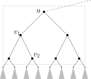
Figure 1: Illustrating $T_{u}(\mathcal{P})$, i.e., the portion of the tree in the dotted box, where $\sqrt{\log n}=3$.

Consider the $i$-th super-level. Let $u$ be any node at the highest level (i.e., the level with the smallest level number) of this super-level. Let $T_{u}(\mathcal{P})$ denote the subtree of $T(\mathcal{P})$ rooted at $u$ without including any node outside the $i$-th super-level (e.g., see Fig. 1 and its corresponding cut-lines and level numbers in Fig. 2). Since $T_{u}(\mathcal{P})$ has $O(\sqrt{\log n})$ levels, $T_{u}(\mathcal{P})$ has $O(2^{\sqrt{\log n}})$ nodes. Recall that $u$ is associated with a subset $V(u)$ of obstacle vertices and a vertical cut-line $l(u)$, and for any vertex $p$ in $V(u)$, if $p$ is horizontally visible to $l(u)$, then its projection point $p_{h}(l(u))$ is a type-2 Steiner point. Each point $p\in V(u)$ defines the following type-3 Steiner points. For each node $v$ in $T_{u}(\mathcal{P})$, if $p$ is horizontally visible to $l(v)$, then its projection point $p_{h}(l(v))$ is a type-3 Steiner point (e.g., see Fig. 2; note that if $p\in V(v)$, then the Steiner point is also a type-2 Steiner point). Hence, $p$ defines $O(2^{\sqrt{\log n}})$ type-3 Steiner points in the $i$-th super-level of $T(\mathcal{P})$. Let $S(p)$ be the set of all type-2 and type-3 Steiner points on the cut-lines of the subtree $T_{u}(\mathcal{P})$ induced by $p$, and let $S(p)$ also contain $p$. In the order of the points in $S(p)$ from left to right, we put an edge in $G_{E}$ connecting every two consecutive points in $S(p)$ (e.g., see Fig. 2). Since the total number of obstacle vertices in $V(u)$ for all nodes $u$ at the same level of $T(\mathcal{P})$ is $n$, the number of type-3 Steiner points thus defined in each super-level is $O(n2^{\sqrt{\log n}})$, and the total number of type-3 Steiner points on all cut-lines in $T(\mathcal{P})$ is $O(n\sqrt{\log n}2^{\sqrt{\log n}})$. The number of edges thus added to $G_{E}$ is also $O(n\sqrt{\log n}2^{\sqrt{\log n}})$.

Hence, the total number of nodes in $G_{E}$ is $O(n\sqrt{\log n}2^{\sqrt{\log n}})$, which is dominated by the number of type-3 Steiner points. We have also defined above some edges in $G_{E}$. The rest of edges in $G_{E}$ are defined similarly as in $G_{old}$. Specifically, first, as in $G_{old}$, for every obstacle vertex $p$, there is an edge $\overline{pq}$ in $G_{E}$ for each $q\in\{p^{l},p^{r},p^{u},p^{d}\}$. Second, as in $G_{old}$, for each obstacle edge $e$, $e$ may contain multiple type-1 Steiner points; the segment connecting each pair of consecutive graph nodes on $e$ defines an edge in $G_{E}$. Third, for each cut-line $l$, every pair of consecutive Steiner points (type-2 or type-3) on $l$ defines an edge in $G_{E}$ if these two points are visible to each other. Clearly, the total number of edges in $G_{E}$ is $O(n\sqrt{\log n}2^{\sqrt{\log n}})$.

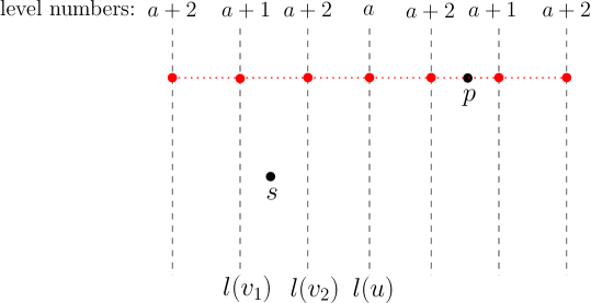
Figure 2: Illustrating the cut-lines and level numbers of the subtree $T_{u}(\mathcal{P})$ in Fig. 1, where $a$ is the level number $ln(u)$ of the node $u$. $p$ is an obstacle vertex. If $p$ is visible to all cut-lines, then the red points are type-2 and type-3 Steiner points defined by $p$ and the (red) dotted segments are the corresponding graph edges.

This finishes the definition of our enhanced graph $G_{E}$, which has $O(n\sqrt{\log n}2^{\sqrt{\log n}})$ nodes and $O(n\sqrt{\log n}2^{\sqrt{\log n}})$ edges. The following lemma gives an algorithm for computing $G_{E}$.

Lemma 1

The enhanced graph $G_{E}$ can be constructed in $O(n\log^{3/2}n2^{\sqrt{\log n}})$ time.

Proof

First of all, all type-1 Steiner points are computed easily in $O(n\log n)$ time, e.g., by using the vertical and horizontal visibility decompositions of $\mathcal{P}$. The edges of $G_{E}$ connecting the obstacle vertices and their corresponding type-1 Steiner points can also be computed. For each obstacle edge $e$, we sort all graph nodes on $e$ and then compute the edges of $G_{E}$ connecting the consecutive nodes on $e$. Since there are $O(n)$ type-1 Steiner points, computing these edges takes $O(n\log n)$ time.

Next, we compute both the type-2 and type-3 Steiner points and their adjacent edges. For this, we need to use the two projection points $p^{l}$ and $p^{r}$ for each obstacle vertex $p$ of $\mathcal{P}$, which have been computed as type-1 Steiner points. Consider an obstacle vertex $p$ in $V(u)$ for a node $u$ at the highest level of a super-level. For each node $v$ in $T_{u}(\mathcal{P})$, we need to determine whether $p$ is horizontally visible to $l(v)$, which can be done in $O(1)$ time since $p^{l}$ and $p^{r}$ are already known. We also need to have a sorted order of all cut-lines in $T_{u}(\mathcal{P})$ from left to right, and this ordered list can be obtained by an in-order traversal of $T_{u}(\mathcal{P})$ in linear time. Therefore, the edges of $G_{E}$ connecting the Steiner points defined by $p$ on consecutive cut-lines in this super-level can be computed in time linear to the number of nodes in $T_{u}(\mathcal{P})$. Since there are $O(n\sqrt{\log n}2^{\sqrt{\log n}})$ type-2 and type-3 Steiner points, computing all such edges takes $O(n\sqrt{\log n}2^{\sqrt{\log n}})$ time.

It remains to compute the graph edges on all cut-lines connecting consecutive Steiner points (if they are visible to each other). This step is done in $O(n\log^{3/2}n2^{\sqrt{\log n}})$ time by a sweeping algorithm, as follows. For each cut-line $l$, we sort the Steiner points on $l$ by their $y$-coordinates, and determine whether every two consecutive Steiner points on $l$ are visible to each other. For this, we sweep a vertical line $L$ from left to right. During the sweeping, we use a balanced binary search tree $T$ to maintain the maximal intervals of $L$ that are in the free space of $\mathcal{P}$ (there are $O(n)$ such intervals). At each obstacle vertex, we update $T$ in $O(\log n)$ time. At each (vertical) cut-line $l$, for every two consecutive Steiner points, we determine whether they are visible to each other in $O(\log n)$ time by checking whether they are in the same maximal interval maintained by $T$. Since there are $O(n\sqrt{\log n}2^{\sqrt{\log n}})$ pairs of consecutive Steiner points on all cut-lines, computing all edges of $G_{E}$ on the cut-lines takes totally $O(n\log^{3/2}n2^{\sqrt{\log n}})$ time. Another approach for computing these edges in $O(n\log^{3/2}n2^{\sqrt{\log n}})$ time is to perform vertical ray-shootings from all Steiner points (we omit the details).

In summary, the enhanced graph $G_{E}$ can be computed in $O(n\log^{3/2}n2^{\sqrt{\log n}})$ time.

3.2 Reducing the Query Time

We use the enhanced graph $G_{E}$ to reduce the query time to $O(\log n)$. Consider two query points $s$ and $t$. One of our key ideas is: We define a new set of gateways for $s$, denoted by $V_{g}(s,G_{E})$, which contains $O(\sqrt{\log n})$ nodes of $G_{E}$, such that for any obstacle vertex $p$ of $\mathcal{P}$, there exists a shortest path from $s$ to $p$ through a gateway of $V_{g}(s,G_{E})$. The set $V_{g}(s,G_{E})$ can be divided into two subsets $V^{1}_{g}(s,G_{E})$ and $V^{2}_{g}(s,G_{E})$, where $V^{1}_{g}(s,G_{E})$ (of size $O(1)$) is exactly the same as $V^{1}_{g}(s,G_{old})$ defined on $G_{old}$ in Section 2. Below, we define the subset $V^{2}_{g}(s,G_{E})$.

Recall that $s$ has $O(\log n)$ projection cut-lines, as defined in Section 2. By definition, $s$ is horizontally visible to all its projection cut-lines. Since $G_{E}$ has more Steiner points than $G_{odd}$, the intuition is that we do not have to include gateways in each projection cut-line of $s$. More specifically, we only need to include gateways in two projection cut-lines in each super-level (one to the left of $s$ and the other to the right of $s$). The details are given below.

We define the relevant projection cut-lines of $s$, as follows. Let $S$ be the set of projection cut-lines of $s$ to the right of $s$. Consider a cut-line $l\in S$ and suppose $l$ is associated with a node $u$ in the $i$-th super-level of the cut-line tree $T(\mathcal{P})$ for some $i$. Then $l$ is a relevant projection cut-line of $s$ if $ln(u)>ln(v)$ (i.e., their level numbers) for every node $v$ with $v\neq u$ in the $i$-th super-level of $T(\mathcal{P})$ such that the cut-line $l(v)$ of $v$ is also in $S$. In other words, $l(u)$ is a relevant projection cut-line of $s$ if $u$ has the largest distance in $T(\mathcal{P})$ from the root among all nodes $v$ in the $i$-th super-level of $T(\mathcal{P})$ whose cut-lines $l(v)$ are in $S$. For example, in Fig. 1 and Fig. 2, suppose $s$ is between the cut-lines $l(v_{1})$ and $l(v_{2})$ and both $l(u)$ and $l(v_{2})$ are horizontally visible to $s$; then among the cut-lines of all nodes in $T_{u}(\mathcal{P})$, only $l(v_{2})$ and $l(u)$ are in $S$, but only $l(v_{2})$ is the relevant projection cut-line of $s$. The relevant projection cut-lines of $s$ to the left of $s$ are defined similarly. Since $s$ has $O(\log n)$ projection cut-lines and any two of them are at different levels of $T(\mathcal{P})$, the number of relevant projection cut-lines of $s$ is $O(\sqrt{\log n})$, i.e., at most two from each super-level of $T(\mathcal{P})$ (one to the left of $s$ and the other to the right of $s$). For each relevant projection cut-line $l$ of $s$, the Steiner point $p$ (if any) immediately above (resp., below) the projection point $s_{h}(l)$ of $s$ on $l$ is in $V^{2}_{g}(s,G_{E})$ if $p$ is visible to $s_{h}(l)$. Thus, $|V^{2}_{g}(s,G_{E})|=O(\sqrt{\log n})$.

$V_{g}(s,G_{E})$ thus defined is of size $O(\sqrt{\log n})$. We also define the gateway edge for each gateway of $V_{g}(s,G_{E})$ and $s$ in the same way as in Section 2. Below, when we say a shortest path from $s$ containing a gateway, we mean the path containing the corresponding gateway edge as well.

Lemma 2

For any obstacle vertex $p$ of $\mathcal{P}$, there exists a shortest path from $s$ to $p$ using $G_{E}$ that contains a gateway of $s$ in $V_{g}(s,G_{E})$.

Proof

Recall that $V_{g}(s,G_{old})$ is the gateway set of $s$ defined on $G_{old}$ in Section 2, and by [6], there exists a shortest path $\pi(s,p)$ from $s$ to $p$ using $G_{old}$ that contains a point $a\in V_{g}(s,G_{old})$.

By the definition of $G_{E}$, if any edge $e$ of $G_{old}$ connecting two nodes $u$ and $v$ is not an edge of $G_{E}$, then $e$ can be viewed as being “divided” into many edges in $G_{E}$ such that the concatenation of these edges is a path from $u$ to $v$ in $G_{E}$ with the same length as $e$. Hence, $\pi(s,p)$ is still a shortest path along $G_{E}$. For any point $a\in V_{g}(s,G_{old})$ that is on a shortest $s$-$p$ path, we call it a via point. If any via point $a$ is in $V^{1}_{g}(s,G_{old})$, then $a$ is in $V_{g}(s,G_{E})$ since $V^{1}_{g}(s,G_{E})=V^{1}_{g}(s,G_{old})$, and we are done. Otherwise, all via points must be in $V^{2}_{g}(s,G_{old})$. If any such via point $a\in V^{2}_{g}(s,G_{old})$ is also in $V^{2}_{g}(s,G_{E})$, then we are done as well. It remains to prove for the case that for every via point $a$, $a\in V^{2}_{g}(s,G_{old})$ and $a\not\in V^{2}_{g}(s,G_{E})$ hold. Recall that every node of $G_{old}$, including each via point $a$, is also a node of $G_{E}$. Below, we find an $xy$-monotone path from $s$ to such a via point $a$ along $G_{E}$ that contains a gateway $b\in V^{2}_{g}(s,G_{E})$. Since any $xy$-monotone path is a shortest path, this gives a shortest $s$-$p$ path (through $a$) containing a gateway $b$ of $s$ in $V_{g}(s,G_{E})$, thus proving the lemma.

Without loss of generality, we assume that $a$ is to the right of $s$ and above $s$ (i.e., $a$ is to the northeast of $s$, see Fig. 3). Suppose $a$ is on the cut-line $l(v)$ of a node $v$ in the $i$-th super-level of $T(\mathcal{P})$. If $l(v)$ is a relevant cut-line of $s$, then there must be a gateway $b$ of $s$ in $V^{2}_{g}(s,G_{E})$ lying in the vertical segment $\overline{s_{h}(l(v))a}$ on $l(v)$ (possibly $b=a$), and thus we are done. Otherwise, $l(v)$ is not a relevant cut-line of $s$, and there exists a relevant cut-line $l(v^{\prime})$ of $s$ to the right of $s$ such that $v^{\prime}$ is in the $i$-th super-level of $T(\mathcal{P})$ and $ln(v^{\prime})>ln(v)$. Next, we show that the sought gateway $b$ lies on $l(v^{\prime})$.

It was shown in [6] (Lemma 3.4) that the level numbers of the projection cut-lines of $s$ to the right of $s$, in the left-to-right order, are decreasing. This observation can also be seen easily by considering the projection cut-lines of $T(\mathcal{P})$ in a top-down manner. Hence, $l(v^{\prime})$ is to the left of $l(v)$ (see Fig. 3). Let $q$ be the obstacle vertex that defines the Steiner point $a$ on $l(v)$. By our definition of Steiner points, $q$ must be in $V(u)$ for the node $u$ that is the highest ancestor of $v$ (and $v^{\prime}$) in the $i$-th super-level. Therefore, if $q$ is horizontally visible to $l(v^{\prime})$, then $q$ also defines a Steiner point on $l(v^{\prime})$. We now show that $q$ is horizontally visible to $l(v^{\prime})$, and for this, it suffices to prove that $a$ is horizontally visible to $l(v^{\prime})$ since $q$ is horizontally visible to $a$. Because $a\in V^{2}_{g}(s,G_{old})$ and no via point is in $V^{1}_{g}(s,G_{old})$, it was shown in [6] that $a$ must be horizontally visible to the vertical line through $s$. Since $l(v^{\prime})$ is between $s$ and $a\in l(v)$, $a$ is also horizontally visible to $l(v^{\prime})$.

Figure 3: Illustrating the proof of Lemma 2: $q$ is the obstacle vertex that defines the Steiner point $a$; $l(v^{\prime})$ is between $s$ and $l(v)$.

Thus, $q$ defines a Steiner point on $l(v^{\prime})$, i.e., the point $q_{h}(l(v^{\prime}))$ (see Fig. 3). By the definition of $V^{2}_{g}(s,G_{E})$, the lowest Steiner point $b$ on $l(v^{\prime})$ above $s$ must be a gateway in $V^{2}_{g}(s,G_{E})$. Note that $b$ may or may not be $q_{h}(l(v^{\prime}))$, but $b$ cannot be higher than $q_{h}(l(v^{\prime}))$. Thus, the concatenation of the gateway edge from $s$ to $b$, $\overline{bq_{h}(l(v^{\prime}))}$, and $\overline{q_{h}(l(v^{\prime}))a}$, which is an $xy$-monotone path from $s$ to $a$ using $G_{E}$, contains the gateway $b$ of $V^{2}_{g}(s,G_{E})$. The lemma thus follows.

Similarly, we define the gateway set $V_{g}(t,G_{E})$ for $t$ in $G_{E}$. The similar result for $t$ as Lemma 2 for $s$ also holds. Thus, we have the following corollary.

Corollary 1

If there exists a shortest $s$-$t$ path through an obstacle vertex of $\mathcal{P}$, then there exists a shortest $s$-$t$ path through a gateway of $s$ in $V_{g}(s,G_{E})$ and a gateway of $t$ in $V_{g}(t,G_{E})$.

Next, we give an algorithm for computing the two gateway sets $V_{g}(s,G_{E})$ and $V_{g}(t,G_{E})$.

Lemma 3

With a preprocessing of $O(n\log^{3/2}n2^{\sqrt{\log n}})$ time and $O(n\sqrt{\log n}2^{\sqrt{\log n}})$ space, we can compute the gateway sets $V_{g}(s,G_{E})$ and $V_{g}(t,G_{E})$ in $O(\log n)$ time for any query points $s$ and $t$.

Proof

We only discuss the case for computing $V_{g}(s,G_{E})$ since $V_{g}(t,G_{E})$ can be computed similarly.

To compute $V^{1}_{g}(s,G_{E})$, it suffices to determine the four projection points $\{s^{l},s^{r},s^{u},s^{d}\}$ of $s$ on $\partial\mathcal{P}$, which can be computed in $O(\log n)$ time by using the horizontal and vertical visibility decompositions of $\mathcal{P}$. These two visibility decompositions can be built in $O(n\log n)$ time by standard sweeping algorithms. After that, we also need to build a point location data structure [17, 31] on each of the two decompositions in additional $O(n)$ time.

To compute $V^{2}_{g}(s,G_{E})$, it might be possible to modify the approach in [6]. However, to explain the approach in [6], we may have to review a number of observations given in [6]. To avoid a tedious discussion, we propose the following algorithm that is simple.

We first obtain the set $S$ of all relevant projection cut-lines of $s$. This can be done in $O(\log n)$ time by following the cut-line tree $T(\mathcal{P})$ from the root and using $s^{l}$ and $s^{r}$ to determine the horizontal visibility of $s$. Note that the cut-lines of $S$ are at some nodes on a path from the root to a leaf. To obtain $V^{2}_{g}(s,G_{E})$, for each cut-line $l\in S$, we need to: (1) find the Steiner point $p$ on $l$ immediately above (resp., below) $s_{h}(l)$, and (2) determine whether $p$ is visible to $s_{h}(l)$.

Consider a cut-line $l\in S$. Let $v_{1}(l)$ and $v_{2}(l)$ be the two gateways of $V^{2}_{g}(s,G_{E})$ on $l$ (if any) such that $v_{1}(l)$ is above $v_{2}(l)$. That is, $v_{1}(l)$ (resp., $v_{2}(l)$) is the Steiner point on $l$ immediately above (resp., below) $s_{h}(l)$ and visible to $s_{h}(l)$. If we maintain a sorted list of all Steiner points on $l$, then $v_{1}(l)$ and $v_{2}(l)$ can be found by binary search on the sorted list. However, there are two issues with this approach. First, if we do binary search on each cut-line of $S$, since $|S|=O(\sqrt{\log n})$, it takes $O(\log^{3/2}n)$ time on all cut-lines of $S$. Second, even if we find $v_{1}(l)$ and $v_{2}(l)$, we still need to check whether $s_{h}(l)$ is visible to them. To resolve these two issues, we take the following approach.

For every Steiner point $p$ on the cut-line $l$, suppose we associate with $p$ its upward and downward projection points $p_{u}$ and $p_{d}$ on $\partial\mathcal{P}$. Then once we find the Steiner point $q$ on $l$ immediately above (resp., below) $s_{h}(l)$, we can determine easily whether $q$ is visible to $s_{h}(l)$ using $q_{u}$ and $q_{d}$; if $q$ is visible to $s_{h}(l)$, then $v_{1}(l)=q$ (resp., $v_{2}(l)=q$), or else $v_{1}(l)$ (resp., $v_{2}(l)$) does not exist. For any Steiner point $p$ on $l$, $p^{l}$ and $p^{r}$ can be found in $O(\log n)$ time by using the vertical visibility decomposition of $\mathcal{P}$. Since there are $O(n\sqrt{\log n}2^{\sqrt{\log n}})$ Steiner points $p$ on all cut-lines of $T(\mathcal{P})$, their projection points $p^{u}$ and $p^{d}$ can be computed in totally $O(n\log^{3/2}n2^{\sqrt{\log n}})$ time.

Next, for each cut-line $l$, we sort all Steiner points on $l$. With this, one can compute all gateways of $V_{g}^{2}(s,G_{E})$ in $O(\log^{2}n)$ time by doing binary search on each relevant projection cut-line of $s$. To reduce the query time to $O(\log n)$, we make use of the fact that all relevant projection cut-lines of $s$ are at the nodes on a path of $T(\mathcal{P})$ from the root to a leaf. We build a fractional cascading structure [4] on the sorted lists of Steiner points on all cut-lines along $T(\mathcal{P})$, such that the searches on all cut-lines at the nodes on any path of $T(\mathcal{P})$ from the root to a leaf take $O(\log n)$ time. Hence, all gateways of $V_{g}^{2}(s,G_{E})$ can be computed in $O(\log n)$ time. Since the total number of Steiner points in the sorted lists of all cut-lines of $T(\mathcal{P})$ is $O(n\sqrt{\log n}2^{\sqrt{\log n}})$, the fractional cascading structure can be built in $O(n\sqrt{\log n}2^{\sqrt{\log n}})$ space and $O(n\log^{3/2}n2^{\sqrt{\log n}})$ time. The lemma thus follows.

Theorem 3.1

We can build a data structure of size $O(n^{2}\cdot\log n\cdot 4^{\sqrt{\log n}})$ in $O(n^{2}\cdot\log^{2}n\cdot 4^{\sqrt{\log n}})$ time that can answer each two-point $L_{1}$ shortest path query in $O(\log n)$ time (i.e., for any two query points $s$ and $t$, the length of a shortest $s$-$t$ path can be found in $O(\log n)$ time and an actual path can be reported in additional time linear to the number of edges of the output path).

Proof

In the preprocessing, we first build the graph $G_{E}$. Then, for each node $v$ of $G_{E}$, we compute a shortest path tree in $G_{E}$ from $v$. We also maintain a shortest path length table such that for any two nodes $u$ and $v$, the shortest $u$-$v$ path length in $G_{E}$ can be obtained in $O(1)$ time. Since $G_{E}$ is of a size $O(n\sqrt{\log n}2^{\sqrt{\log n}})$, computing and maintaining all these shortest path trees in $G_{E}$ take $O(n^{2}\log n4^{\sqrt{\log n}})$ space and $O(n^{2}\log^{2}n4^{\sqrt{\log n}})$ time. We also do the preprocessing for Lemma 3.

Given any two query points $s$ and $t$, we first check whether there is a trivial shortest $s$-$t$ path, as discussed in Section 2, in $O(\log n)$ time by using the algorithm in [6] (with an $O(n\log n)$ time preprocessing). If there is a trivial shortest $s$-$t$ path, then we are done. Otherwise, there must be a shortest $s$-$t$ path that contains an obstacle vertex of $\mathcal{P}$. Then, we first compute the gateway sets $V_{g}(s,G_{E})$ and $V_{g}(t,G_{E})$ in $O(\log n)$ time by Lemma 3. Finally, we determine the shortest $s$-$t$ path length by using the gateway graph as discussed in Section 2, in $O(\log n)$ time, since there are $O(\sqrt{\log n})$ gateways and thus the gateway graph has $O(\sqrt{\log n})$ nodes and $O(\log n)$ edges.

We can also report an actual shortest $s$-$t$ path in additional time linear to the number of edges of the output path by using the shortest path trees of $G_{E}$. This proves the theorem.

4 Reducing the Time and Space Bounds of the Preprocessing

In this section, we improve the preprocessing in Theorem 3.1 to $O(n+h^{2}\cdot\log h\cdot 4^{\sqrt{\log h}})$ space and $O(n+h^{2}\cdot\log^{2}h\cdot 4^{\sqrt{\log h}})$ time, while maintaining the $O(\log n)$ query time. For this, we shall make use of the extended corridor data structure [7, 8, 11, 30], and more importantly, explore a number of new observations, which may be interesting in their own right.

The corridor structure has been used to solve shortest path problems (e.g., [26, 29, 30]), and new concepts like “ocean”, “bays”, and “canals” have been introduced [7, 8, 9, 10, 11, 12], which we refer to as the “extended corridor structure”. This structure is a subdivision of the free space on which algorithms for specific problems rely. While the extended corridor structure itself is relatively simple, the main difficulty is to design efficient algorithms to exploit it. In some sense, the role played by the extended corridor structure is similar to that of triangulations for many geometric algorithms. We briefly review the extended corridor structure in Section 4.1, since our presentation uses many notations introduced in it.

4.1 The Extended Corridor Structure

For simplicity of discussion, we assume that the obstacles of $\mathcal{P}$ are all contained in a rectangle $\mathcal{R}$. Let $\mathcal{F}$ denote the free space in $\mathcal{R}$, and $\mbox{$T\!r\!i$}(\mathcal{F})$ denote a triangulation of $\mathcal{F}$ (see Fig. 5). The line segments of $\mbox{$T\!r\!i$}(\mathcal{F})$ that are not obstacle edges are referred to as diagonals.

Let $G(\mathcal{F})$ denote the dual graph of $\mbox{$T\!r\!i$}(\mathcal{F})$, i.e., each node of $G(\mathcal{F})$ corresponds to a triangle of $\mbox{$T\!r\!i$}(\mathcal{F})$ and each edge connects two nodes corresponding to two triangles sharing a diagonal of $\mbox{$T\!r\!i$}(\mathcal{F})$. Based on $G(\mathcal{F})$, we compute a planar 3-regular graph, denoted by $G^{3}$ (the degree of every node in $G^{3}$ is three), possibly with loops and multi-edges, as follows. First, we remove each degree-one node from $G(\mathcal{F})$ along with its incident edge; repeat this process until no degree-one node remains in the graph. Second, remove every degree-two node from $G(\mathcal{F})$ and replace its two incident edges by a single edge; repeat this process until no degree-two node remains. The resulted graph is $G^{3}$ (see Fig. 5), which has $O(h)$ faces, nodes, and edges [30]. Every node of $G^{3}$ corresponds to a triangle in $\mbox{$T\!r\!i$}(\mathcal{F})$, called a junction triangle (see Fig. 5). The removal of the nodes for all junction triangles from $G^{3}$ results in $O(h)$ corridors, each of which corresponds to an edge of $G^{3}$.

The boundary of each corridor $C$ consists of four parts (see Fig. 5): (1) A boundary portion of an obstacle $P_{i}\in\mathcal{P}$, from a point $a$ to a point $b$; (2) a diagonal of a junction triangle from $b$ to a point $e$ on an obstacle $P_{j}\in\mathcal{P}$ ($P_{i}=P_{j}$ is possible); (3) a boundary portion of the obstacle $P_{j}$ from $e$ to a point $f$; (4) a diagonal of a junction triangle from $f$ to $a$. The corridor $C$ is a simple polygon. Let $\pi(a,b)$ (resp., $\pi(e,f)$) be the Euclidean shortest path from $a$ to $b$ (resp., $e$ to $f$) in $C$. The region $H_{C}$ bounded by $\pi(a,b),\pi(e,f)$, $\overline{be}$, and $\overline{fa}$ is called an hourglass, which is open if $\pi(a,b)\cap\pi(e,f)=\emptyset$ and closed otherwise (see Fig. 5). If $H_{C}$ is open, then both $\pi(a,b)$ and $\pi(e,f)$ are convex chains and are called the sides of $H_{C}$; otherwise, $H_{C}$ consists of two “funnels” and a path $\pi_{C}=\pi(a,b)\cap\pi(e,f)$ joining the two apices of the two funnels, and $\pi_{C}$ is called the corridor path of $C$. The two funnel apices (e.g., $x$ and $y$ in Fig. 5) are called corridor path terminals. Each side of a funnel is also a convex chain.

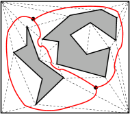
Figure 4: [8, 9] Illustrating a triangulation of the free space among two obstacles and the corridors (indicated by red solid curves). There are two junction triangles marked by a large dot inside each of them, connected by three solid (red) curves. Removing the two junction triangles results in three corridors.

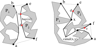
Figure 5: [8, 9] Illustrating an open hourglass (left) and a closed hourglass (right) with a corridor path connecting the apices $x$ and $y$ of the two funnels. The dashed segments are diagonals. The paths $\pi(a,b)$ and $\pi(e,f)$ are shown with thick solid curves. A bay $bay(\overline{cd})$ with gate $\overline{cd}$ (left) and a canal $canal(x,y)$ with gates $\overline{xd}$ and $\overline{yz}$ (right) are also indicated.

Let $\mathcal{M}$ be the union of the $O(h)$ junction triangles, open hourglasses, and funnels. Then $\mathcal{M}\subseteq\mathcal{F}$. We call $\mathcal{M}$ the ocean. Since the sides of open hourglasses and funnels are all convex, the boundary $\partial\mathcal{M}$ of $\mathcal{M}$ consists of $O(h)$ convex chains with a total of $O(n)$ vertices; also, there are $O(h)$ reflex vertices on $\partial\mathcal{M}$, which are corridor path terminals. We further partition the free space $\mathcal{F}\setminus\mathcal{M}$ into regions called bays and canals, as follows.

Consider the hourglass $H_{C}$ of a corridor $C$. If $H_{C}$ is open, then $H_{C}$ has two sides. Let $S_{1}(H_{C})$ be one side of $H_{C}$. The obstacle vertices on $S_{1}(H_{C})$ all lie on the same obstacle, say $P\in\mathcal{P}$. Let $c$ and $d$ be any two consecutive vertices on $S_{1}(H_{C})$ such that $\overline{cd}$ is not an edge of $P$ (e.g., see the left figure in Fig. 5, with $P=P_{j}$). The free region enclosed by $\overline{cd}$ and the boundary portion of $P$ between $c$ and $d$ is called a bay, denoted by $bay(\overline{cd})$. We call $\overline{cd}$ the gate of $bay(\overline{cd})$, which is an edge shared by $bay(\overline{cd})$ and $\mathcal{M}$. If $H_{C}$ is closed, let $x$ and $y$ be the two apices of its two funnels. Consider two consecutive vertices $c$ and $d$ on a side of any funnel such that $\overline{cd}$ is not an obstacle edge. If neither $c$ nor $d$ is a funnel apex, then $c$ and $d$ must lie on the same obstacle and the segment $\overline{cd}$ also defines a bay with that obstacle. However, if $c$ or $d$ is a funnel apex (say, $c=x$), then $c$ and $d$ may lie on different obstacles. If they lie on the same obstacle, then they also define a bay; otherwise, we call $\overline{xd}$ the canal gate at $x=c$ (see Fig. 5). Similarly, there is a canal gate at the other funnel apex $y$, say $\overline{yz}$. Let $P_{i}$ and $P_{j}$ be the two obstacles bounding the hourglass $H_{C}$. The region enclosed by $P_{i}$, $P_{j}$, $\overline{xd}$, and $\overline{yz}$ that contains the corridor path of $H_{C}$ is called a canal, denoted by $canal(x,y)$.

Every bay or canal is a simple polygon. The ocean, bays, and canals together constitute the free space $\mathcal{F}$. While the total number of all bays is $O(n)$, the total number of all canals is $O(h)$.

4.2 Queries in the Ocean $\mathcal{M}$

For any two points $s$ and $t$ in the ocean $\mathcal{M}$, it has been proved that there exists an $L_{1}$ shortest $s$-$t$ path in the free space of the union of $\mathcal{M}$ and all corridor paths [7, 8, 11]. Let $\mathcal{M}^{\prime}$ be the union of $\mathcal{M}$ and all corridor paths. Thus, if $s$ and $t$ are both in $\mathcal{M}$, then there is a shortest $s$-$t$ path in $\mathcal{M}^{\prime}$.

In this subsection, we will first construct a graph $G_{E}(\mathcal{M})$ of size $O(h\cdot\sqrt{\log h}\cdot 2^{\sqrt{\log h}})$ on $\mathcal{M}$, in a similar fashion as $G_{E}$ in Section 3. Using the graph $G_{E}(\mathcal{M})$ and with additional $O(n)$ space, for any query points $s$ and $t$ in $\mathcal{M}$, the shortest path query can be answered in $O(\log n)$ time.

Let $\mathcal{Q}=\mathcal{R}\setminus\mathcal{M}$. Note that $\partial\mathcal{Q}$ is $\partial\mathcal{M}$. Hence, $\partial\mathcal{Q}$ consists of $O(h)$ convex chains with totally $O(n)$ vertices, and $\partial\mathcal{Q}$ also contains $O(h)$ reflex vertices that are corridor path terminals. Since $\mathcal{P}$ has $h$ obstacles, $\mathcal{Q}$ contains at most $h$ connected components and each obstacle of $\mathcal{P}$ is contained in a component of $\mathcal{Q}$. For any point $q$ in $\mathcal{M}$, in this subsection, let $q^{l}$, $q^{r},q^{u}$, and $q^{d}$ denote the leftward, rightward, upward, and downward projection points of $q$ on $\partial\mathcal{Q}$, respectively.

An obstacle vertex $p$ on $\partial\mathcal{Q}$ is said to be extreme if both its incident edges on $\partial\mathcal{Q}$ are on the same side of the vertical or horizontal line through $p$. Let $V_{e}(\mathcal{Q})$ denote the set of all extreme vertices and corridor path terminals of $\mathcal{Q}$. Since $\partial\mathcal{Q}$ consists of $O(h)$ convex chains and $O(h)$ reflex vertices that are corridor path terminals, $|V_{e}(\mathcal{Q})|=O(h)$. We could build a graph on $V_{e}(\mathcal{Q})$ with respect to $\mathcal{Q}$ in a similar way as we built $G_{E}$ on the obstacle vertices of $\mathcal{P}$ in Section 3, and then use this graph to answer queries when both query points are in $\mathcal{M}$. However, in order to handle the general queries (in Section 4.3) for which at least one query point is not in $\mathcal{M}$, we need to consider more points for building the graph. Specifically, let $\mathcal{V}(\mathcal{Q})=\{p^{l},p^{r},p^{u},p^{d}\ |\ p\in V_{e}(\mathcal{Q})\}\cup V_{e}(\mathcal{Q})$, i.e., in addition to $V_{e}(\mathcal{Q})$, $\mathcal{V}(\mathcal{Q})$ also contains the four projections of all points in $V_{e}(\mathcal{Q})$ on $\partial\mathcal{Q}$. Since $|V_{e}(\mathcal{Q})|=O(h)$, $|\mathcal{V}(\mathcal{Q})|=O(h)$.

For each connected component $Q$ of $\mathcal{Q}$, let $\mathcal{V}(Q)$ denote the set of points of $\mathcal{V}(\mathcal{Q})$ on $Q$. Consider any two points $a$ and $b$ of $\mathcal{V}(Q)$ that are consecutive on the boundary $\partial Q$ of $Q$. By the definition of $a$ and $b$, the boundary portion of $\partial Q$ between $a$ and $b$ that contains no other points of $\mathcal{V}(Q)$ must be an $xy$-monotone path (similar results were also given in [7, 8, 11, 26]), and we call it an elementary curve of $\partial Q$. Hence, for any two points on an elementary curve, the portion of the curve between the two points is a shortest path between the two points.

Our goal is to build a graph, denoted by $G_{E}(\mathcal{M})$, on $\mathcal{V}(\mathcal{Q})$ with respect to $\mathcal{Q}$ in a similar way as we built $G_{E}$ in Section 3, and use it to answer queries. To argue the correctness of our approach, we also define a graph $G_{old}(\mathcal{M})$ on $\mathcal{V}(\mathcal{Q})$ and $\mathcal{Q}$ in a similar way as $G_{old}$ on $\mathcal{P}$. Again, $G_{old}(\mathcal{M})$ is only for showing the correctness of our approach based on $G_{E}(\mathcal{M})$ (recall that we use $G_{old}$ to show the correctness of using $G_{E}$). Below, we define $G_{E}(\mathcal{M})$ and $G_{old}(\mathcal{M})$ simultaneously.

We first define their node sets. Each point of $\mathcal{V}(\mathcal{Q})$ defines a node in both graphs. In addition, $G_{old}(\mathcal{M})$ has type-1 and type-2 Steiner points as nodes; $G_{E}(\mathcal{M})$ has type-1, type-2, and type-3 Steiner points as nodes. Such Steiner points are defined using $\mathcal{V}(\mathcal{Q})$ in a similar way as before, but with respect to $\partial\mathcal{Q}$. Specifically, for each point $p\in\mathcal{V}(\mathcal{Q})$, its four projections $p^{l},p^{r},p^{u}$, and $p^{d}$ on $\partial\mathcal{Q}$ are type-1 Steiner points. Let $T(\mathcal{M})$ be the cut-line tree defined on the points of $\mathcal{V}(\mathcal{Q})$, similar to $T(\mathcal{P})$. Each node $u$ of $T(\mathcal{M})$ is associated with a subset $V(u)\subseteq\mathcal{V}(\mathcal{Q})$ and a vertical cut-line $l(u)$ through the median of the $x$-coordinates of the points in $V(u)$. Since $|\mathcal{V}(\mathcal{Q})|=O(h)$, $T(\mathcal{M})$ has $O(\log h)$ levels and $O(\sqrt{\log h})$ super-levels. For every node $u\in T(\mathcal{M})$, for each point $p\in V(u)$, if $p$ is horizontally visible to $l(u)$, then the projection of $p$ on $l(u)$ is a type-2 Steiner point. Also, there are $O(h\sqrt{\log h}2^{\sqrt{\log h}})$ type-3 Steiner points on the cut-lines of $T(\mathcal{M})$, which are defined in a similar way as in Section 3, and we omit the details.

The edge sets of the two graphs are defined similarly as those in $G_{old}$ and $G_{E}$. We only point out the differences here. One big difference is that for each corridor path, since its two terminals define two nodes in both $G_{old}(\mathcal{M})$ and $G_{E}(\mathcal{M})$, $G_{E}(\mathcal{M})$ has an edge connecting these two nodes in both graphs whose weight is the length of the corridor path. Another subtle difference is as follows. In $G_{old}$ and $G_{E}$, for each obstacle edge $e$ of $\mathcal{P}$, both graphs have an edge connecting each pair of consecutive graph nodes on $e$. In contrast, here we consider each individual elementary curve of $\mathcal{Q}$ instead of each individual edge of $\mathcal{Q}$ because not every vertex of $\mathcal{Q}$ defines a node in $G_{old}(\mathcal{M})$ and $G_{E}(\mathcal{M})$. Specifically, consider each elementary curve $\beta$ of $\mathcal{Q}$. Note that the two endpoints of $\beta$ must be in $\mathcal{V}(Q)$ and thus define two nodes in both graphs. For each pair of consecutive graph nodes along $\beta$, we put an edge in both $G_{old}(\mathcal{M})$ and $G_{E}(\mathcal{M})$ whose weight is the length of the portion of $\beta$ between these two points. We then have the following lemma.

Lemma 4

For any two points $u$ and $v$ in $\mathcal{V}(\mathcal{Q})$, a shortest path from $u$ to $v$ in $G_{old}(\mathcal{M})$ (resp., $G_{E}(\mathcal{M})$) corresponds to a shortest path from $u$ to $v$ in the plane.

Proof

We first show that a shortest path from $u$ to $v$ in $G_{old}(\mathcal{M})$ corresponds to a shortest path from $u$ to $v$ in the plane, and then show a shortest path from $u$ to $v$ in $G_{E}(\mathcal{M})$ corresponds to a shortest path from $u$ to $v$ in $G_{old}(\mathcal{M})$. This will prove the lemma.

To show a shortest path from $u$ to $v$ in $G_{old}(\mathcal{M})$ corresponds to a shortest path from $u$ to $v$ in the plane, we will build a new graph $G$ and prove the following: (1) a shortest path from $u$ to $v$ in $G$ corresponds to a shortest path from $u$ to $v$ in $G_{old}(\mathcal{M})$, and (2) a shortest path from $u$ to $v$ in $G$ corresponds to a shortest path from $u$ to $v$ in the plane. Below, to define the graph $G$, we first review some observations that have been discovered before.

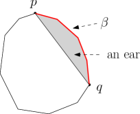
Figure 6: Illustrating an ear bounded by $\overline{pq}$ and an elementary curve $\beta$.

Let $Q$ be any connected component of $\mathcal{Q}$. Consider an elementary curve $\beta$ of $Q$ with endpoints $p$ and $q$. By the definition of elementary curves, the line segment $\overline{pq}$ must be inside $Q$ (similar results were given in [7, 8, 11]). We call the region enclosed by $\beta$ and $\overline{pq}$ an ear of $Q$, $\overline{pq}$ the base of the ear, and $\beta$ the elementary curve of the ear. It is possible that $\beta$ is $\overline{pq}$, in which case the ear is $\overline{pq}$. It is easy to see that the bases of all elementary curves of $Q$ do not intersect except at their endpoints [7, 8, 11]. Hence, if we connect the bases of its elementary curves, we obtain a simple polygon that is contained in $Q$; we call this simple polygon the core of $Q$, denoted by $Q_{core}$. Clearly, the union of $Q_{core}$ and all the ears of $Q$ is $Q$. Denote by $\mathcal{Q}_{core}$ the set of cores of all components of $\mathcal{Q}$. Note that the vertex set of $\mathcal{Q}_{core}$ is $\mathcal{V}(\mathcal{Q})$ and the edges of $\mathcal{Q}_{core}$ are the bases of all ears of $\mathcal{Q}$. Thus, $\mathcal{Q}_{core}$ has $O(h)$ vertices and edges. By the results in [7, 8, 11], for any two points in $\mathcal{M}$, in particular, any two vertices $u$ and $v$ in $\mathcal{V}(\mathcal{Q})$, there is a shortest $u$-$v$ path in the plane that avoids all cores of $\mathcal{Q}_{core}$ and possibly contains corridor paths. More specifically, there exists a shortest path $\pi(u,v)$ from $u$ to $v$ that contains a sequence of vertices of $\mathcal{V}(\mathcal{Q})$, $p_{1},p_{2},\ldots,p_{k}$, in this order, with $u=p_{1}$ and $v=p_{k}$, such that for any two consecutive vertices $p_{i}$ and $p_{i+1}$, $1\leq i\leq k-1$, if $p_{i}$ and $p_{i+1}$ are terminals of the same corridor path, then the entire corridor path is contained in $\pi(u,v)$, or else $\pi(u,v)$ contains the line segment $\overline{p_{i}p_{i+1}}$ which does not intersect the interior of any core in $\mathcal{Q}_{core}$.

We build a graph $G=G_{old}(\mathcal{Q}_{core})$ on $\mathcal{V}(\mathcal{Q})$ with respect to the cores of $\mathcal{Q}$, in the same way as $G_{old}$ on $\mathcal{P}$ in [6, 15, 16], with the only difference that if two nodes of $G$ are terminals of the same corridor path, then there is an extra edge in $G$ connecting these two nodes whose weight is the length of the corridor path. Note that $u$ and $v$ define two nodes in $G$. Based on the above discussion, we claim that the shortest path $\pi(u,v)$ defined above must correspond to a shortest path from $u$ to $v$ in $G$. Indeed, for any $i$, $1\leq i\leq k-1$, if $p_{i}$ and $p_{i+1}$ are terminals of the same corridor path, then recall that $\pi(u,v)$ contains the entire corridor path and there is an edge in $G$ connecting $p_{i}$ and $p_{i+1}$ whose weight is the length of that corridor path; otherwise, $\pi(u,v)$ contains the segment $\overline{p_{i}p_{i+1}}$ and by the proof in [15, 16], there must be a path in $G$ whose length is equal to that of $\overline{p_{i}p_{i+1}}$ since $p_{i}$ is visible to $p_{i+1}$ with respect to the cores of $\mathcal{Q}$. This proves that there is a shortest $u$-$v$ path in $G$ whose length is equal to that of $\pi(u,v)$.

Next, we prove that a shortest $u$-$v$ path in $G$ must correspond to a shortest $u$-$v$ path in $G_{old}(\mathcal{M})$. To make the paper self-contained we give some details below; for complete details, please refer to [26, 7, 8]. Both $G_{old}(\mathcal{M})$ and $G$ are built on $\mathcal{V}(\mathcal{Q})$ in the same way, with the only difference that $G_{old}(\mathcal{M})$ is built with respect to $\mathcal{Q}$ while $G$ is built with respect to $\mathcal{Q}_{core}$. A useful fact is that for any two points $a$ and $b$ on any elementary curve $\beta$, the length of the portion of $\beta$ between $a$ and $b$ is equal to that of the segment $\overline{ab}$ because $\beta$ is $xy$-monotone. Note that the space outside $\mathcal{Q}_{core}$ is the union of the space outside $\mathcal{Q}$ and all ears of $\mathcal{Q}$. Since both graphs have extra edges to connect corridor path terminals, to prove that a shortest $u$-$v$ path in $G$ corresponds to a shortest $u$-$v$ path in $G_{old}(\mathcal{M})$, based on the analysis in [15, 16], we only need to show the following: For any two vertices $a$ and $b$ of $\mathcal{V}(\mathcal{Q})$ visible to each other with respect to $\mathcal{Q}_{core}$ such that no other vertices of $\mathcal{V}(\mathcal{Q})$ than $a$ and $b$ are in the axis-parallel rectangle $R(a,b)$ that has $\overline{ab}$ as a diagonal, there must be an $xy$-monotone path between $a$ and $b$ in $G_{old}(\mathcal{M})$. Note that $a$ may not be visible to $b$ with respect to $\mathcal{Q}$.

By the construction of the graph $G$ [15, 16], there must be an $xy$-monotone path from $a$ to $b$ in $G$, for which there are two possible cases. Below, we prove in each case there is also an $xy$-monotone path from $a$ to $b$ in $G_{old}(\mathcal{M})$. Without loss of generality, we assume $b$ is to the northeast of $a$.

1. Case 1. If any core of $\mathcal{Q}_{core}$ intersects the interior of the rectangle $R(a,b)$, then as shown in [15, 16], either the rightward projection of $a$ on $\partial\mathcal{Q}_{core}$ and the downward projection of $b$ on $\partial\mathcal{Q}_{core}$ are both on the same edge of $\partial\mathcal{Q}_{core}$ that intersects $R(a,b)$ (e.g., see Fig. 8), or the upward projection of $a$ on $\partial\mathcal{Q}_{core}$ and the leftward projection of $b$ on $\partial\mathcal{Q}_{core}$ are both on the same edge of $\partial\mathcal{Q}_{core}$ that intersects $R(a,b)$. Here, we assume that the former case occurs. Let $a_{1}$ be the rightward projection of $a$ on $\partial\mathcal{Q}_{core}$ and $b_{1}$ be the downward projection of $b$ on $\partial\mathcal{Q}_{core}$, and $\overline{a_{2}b_{2}}$ be the edge of $\mathcal{Q}_{core}$ that contains both $a_{1}$ and $b_{1}$. By the construction of $G$, there is an $xy$-monotone path from $a$ to $b$ consisting of $\overline{aa_{1}}\cup\overline{a_{1}b_{1}}\cup\overline{b_{1}b}$. Below, we show that there is also an $xy$-monotone path from $a$ to $b$ in $G_{old}(\mathcal{M})$.

   Let $ear(\overline{a_{2}b_{2}})$ be the ear of $\mathcal{Q}$ whose base is $\overline{a_{2}b_{2}}$. Let $\beta$ be the elementary curve of $ear(\overline{a_{2}b_{2}})$. Since no vertex of $\mathcal{V}(\mathcal{Q})-\{a,b\}$ is in $R(a,b)$ and all extreme points of $\mathcal{Q}$ are in $\mathcal{V}(\mathcal{Q})$, the rightward projection of $a$ on $\partial\mathcal{Q}$ and the downward projection of $b$ on $\partial\mathcal{Q}$ must be both on $\beta$ (e.g., see Fig. 8); we denote these two projection points by $a_{3}$ and $b_{3}$, respectively. By the construction of $G_{old}(\mathcal{M})$, there must be an $xy$-monotone path from $a$ to $b$ in $G_{old}(\mathcal{M})$ that is a concatenation of $\overline{aa_{3}}$, the portion of $\beta$ between $a_{3}$ and $b_{3}$, and $\overline{b_{3}b}$ (note that $a_{3}$ is a type-1 Steiner point defined by $a$ and $b_{3}$ is a type-1 Steiner point defined by $b$ in $G_{old}(\mathcal{M})$).

   

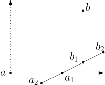
   Figure 7: Illustrating the proof of Lemma 4: $a_{1}$ is the rightward projection of $a$ on $\partial\mathcal{Q}_{core}$ and $b_{1}$ is the downward projection of $b$ on $\partial\mathcal{Q}_{core}$.

   

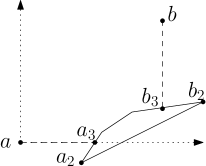
   Figure 8: Illustrating the proof of Lemma 4: $a_{3}$ is the rightward projection of $a$ on $\partial\mathcal{Q}$ and $b_{3}$ is the downward projection of $b$ on $\partial\mathcal{Q}$. Both $a_{3}$ and $b_{3}$ must be on the same elementary curve $\beta$.

2. Case 2. If no core of $\mathcal{Q}_{core}$ intersects the interior of the rectangle $R(a,b)$, then by the construction of $G$, there must be a cut-line $l$ between $a$ and $b$ such that on $l$, $a$ defines a Steiner point $a_{h}(l)$ and $b$ defines a Steiner point $b_{h}(l)$ (e.g., see Fig. 10). Thus, there is an $xy$-monotone path from $a$ to $b$ in $G$ consisting of $\overline{aa_{h}(l)}\cup\overline{a_{h}(l)b_{h}(l)}\cup\overline{b_{h}(l)b}$. Below, we show that there is also an $xy$-monotone path from $a$ to $b$ in $G_{old}(\mathcal{M})$.

   

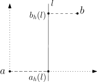
   Figure 9: Illustrating the proof of Lemma 4: $a_{h}(l)$ is the rightward projection of $a$ on $l$ and $b_{h}(l)$ is the leftward projection of $b$ on $l$.

   

   Figure 10: Illustrating the proof of Lemma 4: $a_{1}$ is the rightward projection of $a$ on $\partial\mathcal{Q}$ and $b_{1}$ is the downward projection of $b$ on $\partial\mathcal{Q}$. Both $a_{1}$ and $b_{1}$ must be on the same elementary curve $\beta$.

   Since both $G$ and $G_{old}(\mathcal{M})$ are built on $\mathcal{V}(\mathcal{Q})$, they have the same cut-line tree. Hence, the cut-line $l$ still exists in $G_{old}(\mathcal{M})$. If both $a$ and $b$ are horizontally visible to $l$, then they still define Steiner points on $l$ and consequently there is also an $xy$-monotone path from $a$ to $b$ in $G_{old}(\mathcal{M})$. Otherwise, we assume that $a$ is not horizontally visible to $l$. Let $a_{1}$ be the rightward projection of $a$ on $\partial\mathcal{Q}$ (see Fig. 10). Hence, $a_{1}$ must be between $l$ and $a$. Let $\beta$ be the elementary curve that contains $a_{1}$. Thus, $\beta$ intersects the lower edge of $R(a,b)$ at $a_{1}$. Since $R(a,b)$ does not contain any point of $\mathcal{V}(\mathcal{Q})-\{a,b\}$, the two endpoints of $\beta$ are not in $R(a,b)$ and thus the downward projection of $b$ on $\partial\mathcal{Q}$, denoted by $b_{1}$, must be on $\beta$ as well. By the construction of $G_{old}(\mathcal{M})$, there must be an $xy$-monotone path from $a$ to $b$ in $G_{old}(\mathcal{M})$ that is the concatenation of $\overline{aa_{1}}$, the portion of $\beta$ between $a_{1}$ and $b_{1}$, and $\overline{b_{1}b}$.

The above arguments prove that a shortest path from $u$ to $v$ in $G_{old}(\mathcal{M})$ corresponds to a shortest path from $u$ to $v$ in the plane.

It remains to show that a shortest $u$-$v$ path in $G_{old}(\mathcal{M})$ corresponds to a shortest $u$-$v$ path in $G_{E}(\mathcal{M})$. This can be seen easily since for any edge $e=\overline{pq}$ in $G_{old}(\mathcal{M})$, if $e$ is not in $G_{E}(\mathcal{M})$, then $e$ is “divided” into many edges in $G_{E}(\mathcal{M})$ such that their concatenation is a path from $p$ to $q$.

The lemma thus follows.

The next lemma gives an algorithm for computing the graph $G_{E}(\mathcal{M})$.

Lemma 5

The graph $G_{E}(\mathcal{M})$ can be computed in $O(n+h\log^{3/2}h2^{\sqrt{\log h}})$ time.

Proof

The algorithm for constructing $G_{E}(\mathcal{M})$ is similar to that for $G_{E}$ in Lemma 1. As a preprocessing, the free space $\mathcal{F}$ can be triangulated in $O(n+h\log^{1+\epsilon}h)$ time for any constant $\epsilon>0$ [2], after which computing the extended corridor structure, in particular, takes $O(n+h\log h)$ time [7, 8, 11]. Consequently, we obtain $\mathcal{Q}$ and the vertex set $\mathcal{V}(\mathcal{Q})$. All corridor paths are also available.

First, we compute the four projections of each point of $\mathcal{V}(\mathcal{Q})$ on $\partial\mathcal{Q}$ as type-1 Steiner points, which can be done after we compute the vertical and horizontal visibility decompositions of $\mathcal{Q}$ in $O(n+h\log^{1+\epsilon}h)$ time [2]. The graph edges for connecting each point of $\mathcal{V}(\mathcal{Q})$ to its four projection points on $\partial\mathcal{Q}$ can be obtained as well.

Next, we compute the type-2 and type-3 Steiner points and the corresponding graph edges connecting these Steiner points. Since $|\mathcal{V}(\mathcal{Q})|=O(h)$, the cut-line tree $T(\mathcal{M})$ can be computed in $O(h\log h)$ time. Then, we determine the Steiner points on the cut-lines by traversing the tree $T(\mathcal{M})$ from top to bottom in a similar way as in Lemma 1. Since we have obtained the four projection points for each point of $\mathcal{V}(\mathcal{Q})$, computing all Steiner points on the cut-lines takes $O(h\sqrt{\log h}2^{\sqrt{\log h}})$ time. Their corresponding edges can be computed in $O(h\log^{3/2}h2^{\sqrt{\log h}}\log n)$ time.

It remains to compute the graph edges of $G_{E}(\mathcal{M})$ connecting consecutive graph nodes on each elementary curve of $\mathcal{Q}$ and the graph edges connecting every two consecutive Steiner points (if they are visible to each other) on each cut-line.

On each connected component $Q$ of $\mathcal{Q}$, we could compute a sorted list of all Steiner points and the points of $\mathcal{V}(Q)$ by sorting all these points and all obstacle vertices of $Q$ along $\partial Q$. But that would take $O(n\log n)$ time in total because there are $O(n)$ obstacle vertices on all components of $\mathcal{Q}$. To do better, we take the following approach. For each elementary curve $\beta$, we sort all Steiner points on $\beta$ by either their $x$-coordinates or $y$-coordinates. Since $\beta$ is $xy$-monotone, such an order is also an order along $\beta$. Then, we merge the Steiner points thus ordered with the obstacle vertices on $\beta$, in linear time. Since there are $O(h)$ Steiner points on $\partial\mathcal{Q}$, it takes totally $O(n+h\log h)$ time to sort the Steiner points and obstacle vertices on all elementary curves of $\mathcal{Q}$. After that, the edges of $G_{E}(\mathcal{M})$ on all elementary curves can be computed immediately.

We now compute the graph edges on the cut-lines connecting consecutive Steiner points. We first sort all Steiner points on each cut-line. This sorting takes $O(h\log^{3/2}h2^{\sqrt{\log n}})$ time for all cut-lines. For each pair of consecutive Steiner points $p$ and $q$ on every cut-line, we determine whether $p$ is visible to $q$ by checking whether the upward projections of $p$ and $q$ on $\partial\mathcal{Q}$ are equal, and these upward projections can be performed in $O(\log n)$ time using the vertical visibility decomposition of $\mathcal{Q}$. Hence, the graph edges on all cut-lines are computed in $O(h\sqrt{\log h}2^{\sqrt{\log h}}\cdot\log n)$ time.

In summary, we can compute the graph $G_{E}(\mathcal{M})$ in $O(n+h\sqrt{\log h}2^{\sqrt{\log h}}\cdot\log n)$ time. Note that $n+h\sqrt{\log h}2^{\sqrt{\log h}}\cdot\log n=O(n+h\log^{3/2}h2^{\sqrt{\log h}})$. The lemma thus follows.

Consider any two query points $s$ and $t$ in the ocean $\mathcal{M}$. We define the gateway sets $V_{g}(s,G_{E}(\mathcal{M}))$ for $s$ and $V_{g}(t,G_{E}(\mathcal{M}))$ for $t$ on $G_{E}(\mathcal{M})$, as follows. We only discuss $V_{g}(s,G_{E}(\mathcal{M}))$; $V_{g}(t,G_{E}(\mathcal{M}))$ is similar. The definition of $V_{g}(s,G_{E}(\mathcal{M}))$ is very similar to that of $V_{g}(s,G_{E})$, with only slight differences. Specifically, $V_{g}(s,G_{E}(\mathcal{M}))$ has two subsets $V^{1}_{g}(s,G_{E}(\mathcal{M}))$ and $V^{2}_{g}(s,G_{E}(\mathcal{M}))$. $V^{2}_{g}(s,G_{E}(\mathcal{M}))$ is defined in the same way as $V^{2}_{g}(s,G_{E})$, and thus $|V^{2}_{g}(s,G_{E}(\mathcal{M}))|=O(\sqrt{\log h})$. $V^{1}_{g}(s,G_{E}(\mathcal{M}))$ is defined with respect to the elementary curves of $\mathcal{Q}$, as follows. Let $q$ be the rightward projection point of $s$ on $\partial\mathcal{Q}$. Suppose $q$ is on the elementary curve $\beta$ and $p_{1}$ and $p_{2}$ are the two nodes of $G_{E}(\mathcal{M})$ on $\beta$ adjacent to $q$. Then $p_{1}$ and $p_{2}$ are in $V^{1}_{g}(s,G_{E}(\mathcal{M}))$, and for each $p\in\{p_{1},p_{2}\}$, we define a gateway edge from $s$ to $p$ consisting of $\overline{sq}$ and the portion of $\beta$ between $q$ and $p$. Similarly, for each of the leftward, upward, and downward projections of $s$ on $\partial\mathcal{Q}$, there are at most two gateways in $V^{1}_{g}(s,G_{E}(\mathcal{M}))$.

The next lemma shows that the gateways of $V_{g}(s,G_{E}(\mathcal{M}))$ “control” the shortest paths from $s$ to all points of $\mathcal{V}(\mathcal{Q})$.

Lemma 6

For any point $p$ of $\mathcal{V}(\mathcal{Q})$, there exists a shortest path from $s$ to $p$ using $G_{E}(\mathcal{M})$ that contains a gateway of $s$ in $V_{g}(s,G_{E}(\mathcal{M}))$.

Proof

We define a gateway set $V_{g}(s,G_{old}(\mathcal{M}))$ for $s$ on the graph $G_{old}(\mathcal{M})$, as follows. The set $V_{g}(s,G_{old}(\mathcal{M}))$ has two subsets $V^{1}_{g}(s,G_{old}(\mathcal{M}))$ and $V^{2}_{g}(s,G_{old}(\mathcal{M}))$. The first subset $V^{1}_{g}(s,G_{old}(\mathcal{M}))$ is exactly the same as $V^{1}_{g}(s,G_{E}(\mathcal{M}))$, and the second subset $V^{2}_{g}(s,G_{old}(\mathcal{M}))$ contains gateways on the cut-lines of $T(\mathcal{M})$, which are defined similarly as $V^{2}_{g}(s,G_{old})$ on $G_{old}$ and $T(\mathcal{P})$, discussed in Section 2. Note that the gateways in $V_{g}(s,G_{old}(\mathcal{M}))$ are exactly those nodes of $G_{old}(\mathcal{M})$ that are adjacent to $s$ if we “insert” $s$ into the graph $G_{old}(\mathcal{M})$ (similar arguments were used for $V_{g}(s,G_{old})$ in [6]). Hence, there exists a shortest path from $s$ to $p$ using $G_{old}(\mathcal{M})$ that contains a gateway of $s$ in $V_{g}(s,G_{old}(\mathcal{M}))$.

Since the graph $G_{E}(\mathcal{M})$ is defined analogously as $G_{E}$ and $G_{old}(\mathcal{M})$ is defined analogously as $G_{old}$, by using a similar analysis as in the proof of Lemma 2, we can show that there exists a shortest path from $s$ to $p$ using $G_{E}(\mathcal{M})$ that contains a gateway of $s$ in $V_{g}(s,G_{E}(\mathcal{M}))$. We omit the details. The lemma thus follows.

Similar results also hold for the gateway set $V_{g}(t,G_{E}(\mathcal{M}))$ of $t$. We have the following corollary.

Corollary 2

If there exists a shortest $s$-$t$ path through a point of $\mathcal{V}(\mathcal{Q})$, then there exists a shortest $s$-$t$ path through a gateway of $s$ in $V_{g}(s,G_{E}(\mathcal{M}))$ and a gateway of $t$ in $V_{g}(t,G_{E}(\mathcal{M}))$.

The following lemma gives an algorithm for computing the gateways.

Lemma 7

With a preprocessing of $O(n+h\cdot\log^{3/2}h\cdot 2^{\sqrt{\log h}})$ time and $O(n+h\cdot\sqrt{\log h}\cdot 2^{\sqrt{\log h}})$ space, the gateway sets $V_{g}(s,G_{E}(\mathcal{M}))$ and $V_{g}(t,G_{E}(\mathcal{M}))$ can be computed in $O(\log n)$ time for any two query points $s$ and $t$ in $\mathcal{M}$.

Proof

The algorithm is similar to that for Lemma 3; we only point out the differences. We discuss our algorithm only for computing $V_{g}(s,G_{E}(\mathcal{M}))$; the case for $V_{g}(t,G_{E}(\mathcal{M}))$ is similar.

To compute $V^{1}_{g}(s,G_{E}(\mathcal{M}))$, we build the horizontal and vertical visibility decompositions of $\mathcal{Q}$. Then, the four projections of $s$ on $\partial\mathcal{Q}$ can be determined in $O(\log n)$ time. Consider any such projection $p$ of $s$. Suppose $p$ is on an elementary curve $\beta$. We need to determine the two nodes of $G_{E}(\mathcal{M})$ on $\beta$ adjacent to $p$, which are gateways of $V^{1}_{g}(s,G_{E}(\mathcal{M}))$. We maintain a sorted list of all nodes of $G_{E}(\mathcal{M})$ on $\beta$, and do binary search to find these two gateways of $s$ on $\beta$ in this sorted list by using only the $y$-coordinates (or the $x$-coordinates) of the nodes since $\beta$ is $xy$-monotone. Also, since $\beta$ is $xy$-monotone, for any two points $q$ and $q^{\prime}$ on $\beta$, the length of the portion of $\beta$ between $q$ and $q^{\prime}$ is equal to the length of $\overline{qq^{\prime}}$. Hence, after these two gateways of $s$ on $\beta$ are found, the lengths of the two gateway edges from $s$ to them can be computed in constant time. Since $V^{1}_{g}(s,G_{E}(\mathcal{M}))$ has $O(1)$ gateways, $V^{1}_{g}(s,G_{E}(\mathcal{M}))$ can be computed in $O(\log n)$ time.

To compute $V^{2}_{g}(s,G_{E}(\mathcal{M}))$, we take the same approach as for Lemma 3. In the preprocessing, for every cut-line $l$, we maintain a sorted list of all Steiner points on $l$, and associate with each such Steiner point its upward and downward projections on $\partial\mathcal{Q}$. Computing these projections for each Steiner point takes $O(\log n)$ time. Then we build a fractional cascading data structure [4] for the sorted lists of Steiner points on all cut-lines along the cut-line tree $T(\mathcal{M})$. Using this fractional cascading data structure, the gateway set $V^{2}_{g}(s,G_{E}(\mathcal{M}))$ can be computed in $O(\log h)$ time.

The preprocessing takes totally $O(n+h\sqrt{\log h}2^{\sqrt{\log h}}\log n)$ time and $O(n+h\sqrt{\log h}2^{\sqrt{\log h}})$ space. Note that $n+h\sqrt{\log h}2^{\sqrt{\log h}}\log n=O(n+h\log^{3/2}h2^{\sqrt{\log h}})$. The lemma thus follows.

We summarize our algorithm in Lemma 8 below for the case when both query points are in $\mathcal{M}$.

Lemma 8

With a preprocessing of $O(n+h^{2}\log^{2}h4^{\sqrt{\log h}})$ time and $O(n+h^{2}\log h4^{\sqrt{\log h}})$ space, each two-point query can be answered in $O(\log n)$ time for any two query points in the ocean $\mathcal{M}$.

Proof

In the preprocessing, we build the graph $G_{E}(\mathcal{M})$, and for each node $v$ of $G_{E}(\mathcal{M})$, compute a shortest path tree in $G_{E}(\mathcal{M})$ from $v$. We maintain a shortest path length table such that for any two nodes $u$ and $v$ in $G_{E}(\mathcal{M})$, the shortest path length between $u$ and $v$ can be found in $O(1)$ time. Since $G_{E}(\mathcal{M})$ has $O(h\sqrt{\log h}2^{\sqrt{\log h}})$ nodes and edges, computing and maintaining all shortest path trees in $G_{E}(\mathcal{M})$ take $O(h^{2}\log h4^{\sqrt{\log h}})$ space and $O(h^{2}\log^{2}h4^{\sqrt{\log h}})$ time.

To report an actual shortest path in the plane in time linear to the number of edges of the output path, we need to maintain additional information. Consider an elementary curve $\beta$ of $\mathcal{Q}$. Let $u$ and $v$ be two consecutive nodes of $G_{E}(\mathcal{M})$ on $\beta$. By our definition of $G_{E}(\mathcal{M})$, there is an edge $(u,v)$ in $G_{E}(\mathcal{M})$. If the edge $(u,v)$ is contained in our output path, we need to report all obstacle vertices and edges of $\beta$ between $u$ and $v$. For this, on each elementary curve $\beta$, we explicitly maintain a list of obstacle edge between each pair of consecutive nodes of $G_{E}(\mathcal{M})$ along $\beta$. Since the total number of nodes of $G_{E}(\mathcal{M})$ on all elementary curves is $O(h)$ and the total number of obstacle vertices of $\mathcal{Q}$ is $O(n)$, maintaining such edge lists for all elementary curves takes $O(n)$ space.

In addition, we also perform the preprocessing for Lemma 7.

The overall preprocessing takes $O(n+h^{2}\log^{2}h4^{\sqrt{\log h}})$ time and $O(n+h^{2}\log h4^{\sqrt{\log h}})$ space.

Now consider any two query points $s$ and $t$ in $\mathcal{M}$. As for Theorem 3.1, we first check whether there exists a trivial shortest $s$-$t$ path. But trivial shortest paths here are defined with respect to the elementary curves of $\mathcal{Q}$ instead of the obstacle edges of $\mathcal{P}$. For example, consider $s^{r}$ (i.e., the rightward projection of $s$ on $\partial\mathcal{Q}$) and $t^{d}$. If $\overline{ss^{r}}$ intersects $\overline{tt^{d}}$, then there is a trivial shortest $s$-$t$ path $\overline{sq}\cup\overline{qt}$, where $q=\overline{ss^{r}}\cap\overline{tt^{d}}$; otherwise, if $s^{r}$ and $t^{d}$ are both on the same elementary curve $\beta$ of $\mathcal{Q}$, then there is a trivial shortest $s$-$t$ path which is the concatenation of $\overline{ss^{r}}$, the portion of $\beta$ between $s^{r}$ and $t^{d}$, and $\overline{t^{d}t}$. Similarly, trivial shortest $s$-$t$ paths are also defined by other projections of $s$ and $t$ on $\partial\mathcal{Q}$.

We can determine whether there exists a trivial shortest $s$-$t$ path in $O(\log n)$ time by using the vertical and horizontal decompositions of $\mathcal{Q}$ to compute the four projection points of $s$ and $t$ on $\partial\mathcal{Q}$. If yes, we find such a shortest path in additional time linear to the number of edges of the output path. Note that for the case, e.g., when $s^{r}$ and $t^{d}$ are both on the same elementary curve $\beta$, the output path may not be of $O(1)$ size since there may be multiple obstacle vertices on the portion of $\beta$ between $s^{r}$ and $t^{d}$; but we can still output such a path in linear time by using the edge lists we maintain on each elementary curve. Below, we assume there is no trivial shortest $s$-$t$ path.

By using the cores of $\mathcal{Q}$ in the proof of Lemma 4 and a similar analysis as in [6], we can show that there must be a shortest $s$-$t$ path that contains at least one point of $\mathcal{V}(\mathcal{Q})$. By Corollary 2, there exists a shortest $s$-$t$ path through a gateway of $s$ and a gateway of $t$ in $G_{E}(\mathcal{M})$. Using Lemma 7, we compute the two gateway sets $V_{g}(s,G_{E}(\mathcal{M}))$ and $V_{g}(t,G_{E}(\mathcal{M}))$. By building a gateway graph for $s$ and $t$ as in Theorem 3.1, we can compute the length of a shortest $s$-$t$ path in $O(\log h)$ time since $|V_{g}(s,G_{E}(\mathcal{M}))|=O(\sqrt{\log h})$, $|V_{g}(t,G_{E}(\mathcal{M}))|=O(\sqrt{\log h})$, and thus the gateway graph has $O(\sqrt{\log h})$ nodes and $O(\log h)$ edges. An actual path can then be reported in additional time linear to the number of edges of the output path, by using the shortest path trees of $G_{E}(\mathcal{M})$ and the edge lists maintained on the elementary curves, as discussed above. The lemma thus follows.

4.3 The General Queries

In this section, we show how to handle the general queries in which at least one query point is not in $\mathcal{M}$. Without loss of generality, we assume that $s$ is in a bay or a canal, denoted by $B$. We first focus on the case when $B$ is a bay. The case when $B$ is a canal can be handled by similar techniques although it is a little more complicated since each canal has two gates. The point $t$ can be in $B$, $\mathcal{M}$, or another bay or canal, and we discuss these three cases below. Let $g$ denote the gate of $B$.

As an overview of our approach, we characterize the different possible ways that a shortest $s$-$t$ path may cross the gate $g$, show how to find such a possible path for each way, and finally compute all possible “candidate” paths and select the one with the smallest path length as our solution.

4.3.1 The Query Point $t$ is in $B$

When the query point $t$ is in $B$, we have the following lemma.

Lemma 9

If $B$ is a bay and $t\in B$, then there exists a shortest $s$-$t$ path in $B$.

Proof

Let $\pi$ be any shortest $s$-$t$ path in the plane. If $\pi$ is in $B$, then we are done. Otherwise, $\pi$ must intersect the only gate $g$ of $B$; further, since both $s$ and $t$ are in $B$, if $\pi$ exits from $B$ (through $g$), then it must enter $B$ again (through $g$ as well). Let $p$ be the first point on $g$ encountered as going from $s$ to $t$ along $\pi$ and let $q$ be the last such point on $g$. Let $\pi^{\prime}$ be the $s$-$t$ path obtained by replacing the portion of $\pi$ between $p$ and $q$ by $\overline{pq}\subseteq g$. Note that $\pi^{\prime}$ is in $B$. Since $\overline{pq}$ is a shortest path from $p$ to $q$, $\pi^{\prime}$ is also a shortest $s$-$t$ path. The lemma thus follows.

To handle the case of $t\in B$, in the preprocessing, we build a data structure for two-point Euclidean shortest path queries in $B$, denoted by $\mathcal{D}(B)$, in $O(|B|)$ time and space [19]. Since a Euclidean shortest path in any simple polygon is also an $L_{1}$ shortest path and $B$ is a simple polygon, for $t\in B$, we can use $\mathcal{D}(B)$ to answer the shortest $s$-$t$ path query in $B$ in $O(\log n)$ time.

4.3.2 The Query Point $t$ is in $\mathcal{M}$

If the query point $t$ is in $\mathcal{M}$, then a shortest $s$-$t$ path must cross the gate $g$ of $B$. A main difficulty for answering the general queries is to deal with this case. More specifically, we already have a graph $G_{E}(\mathcal{M})$ on $\mathcal{M}$, and our goal is to design a mechanism to connect the bay $B$ with $G_{E}(\mathcal{M})$ through the gate $g$, so that it can capture the shortest path information in the union of $B$ and $\mathcal{M}^{\prime}$ (recall that $\mathcal{M}^{\prime}$ is the union of $\mathcal{M}$ and all corridor paths).

We begin with some observations on how a shortest $s$-$t$ path may cross $g$. Without loss of generality, we assume that $g$ has a positive slope and the interior of $B$ on $g$ is above $g$. Let $a_{1}$ and $a_{2}$ be the two endpoints of $g$ such that $a_{1}$ is higher than $a_{2}$ (see Fig. 11). Let $\pi(s,a_{1})$ (resp., $\pi(s,a_{2})$) be the Euclidean shortest path in $B$ from $s$ to $a_{1}$ (resp., $a_{2}$). Let $z^{\prime}$ be the farthest point from $s$ on $\pi(s,a_{1})\cap\pi(s,a_{2})$ (possibly $z^{\prime}=s$). Let $\pi(z^{\prime},a_{1})$ (resp., $\pi(z^{\prime},a_{2})$) be the subpath of $\pi(s,a_{1})$ (resp., $\pi(s,a_{2})$) between $z^{\prime}$ and $a_{1}$ (resp., $a_{2}$). It is well known that both $\pi(z^{\prime},a_{1})$ and $\pi(z^{\prime},a_{2})$ are convex chains [20, 33], and the region enclosed by $\pi(z^{\prime},a_{1})$, $\pi(z^{\prime},a_{2})$, and $g$ in $B$ is a “funnel” with $z^{\prime}$ as the apex and $g$ as the base (see Fig. 11). Let $F$ denote this funnel and $\partial F$ denote its boundary.

We define four special points $z^{\prime}_{1},z^{\prime}_{2},z_{1}$, and $z_{2}$ (see Fig. 11). Suppose we move along $\pi(z^{\prime},a_{1})$ from $z^{\prime}$; let $z_{1}^{\prime}$ be the first point on $\pi(z^{\prime},a_{1})$ we encounter that is horizontally visible to $g=\overline{a_{1}a_{2}}$. Similarly, as moving along $\pi(z^{\prime},a_{2})$ from $z^{\prime}$, let $z_{2}^{\prime}$ be the first point on $\pi(z^{\prime},a_{2})$ encountered that is vertically visible to $g$. Note that in some cases $z_{1}^{\prime}$ (resp., $z^{\prime}_{2}$) can be $z^{\prime}$, $a_{1}$, or $a_{2}$. Let $z_{1}$ be the horizontal projection of $z^{\prime}_{1}$ on $g$ and $z_{2}$ be the vertical projection of $z^{\prime}_{2}$ on $g$ (see Fig. 11).

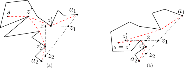
Figure 11: Illustrating the definitions of $z^{\prime},z^{\prime}_{1},z^{\prime}_{2},z,z_{1}$, and $z_{2}$. In (a), $\overline{z_{1}z_{1}^{\prime}}$ is tangent to $\pi(z^{\prime},a_{1})$ (at $z_{1}^{\prime}$); in (b), $\overline{z_{1}z_{1}^{\prime}}$ is tangent to $\pi(z^{\prime},a_{2})$.

The points $z_{1}$ and $z_{2}$ are particularly useful. We first have the following observation.

Observation 1

The point $z_{1}$ is above $z_{2}$, i.e., the $y$-coordinate of $z_{1}$ is no smaller than that of $z_{2}$.

Proof

If $z^{\prime}$ is either $a_{1}$ or $a_{2}$, then by their definitions, we have $z_{1}=z_{2}=z_{1}^{\prime}=z_{2}^{\prime}=z^{\prime}$ and the observation trivially holds. Suppose $z^{\prime}$ is neither $a_{1}$ nor $a_{2}$. If $z_{1}=a_{1}$, then the observation also holds since $a_{1}$ is the highest point on $g$. We assume $z_{1}\neq a_{1}$, which implies $z_{1}^{\prime}\neq a_{1}$.

Let $\pi(z_{1}^{\prime},a_{1})$ be the portion of $\pi(z^{\prime},a_{1})$ between $z_{1}^{\prime}$ and $a_{1}$. Note that the “pseudo-triangular” region enclosed by $\overline{a_{1}z_{1}}$, $\overline{z_{1}z_{1}^{\prime}}$, and $\pi(z_{1}^{\prime},a_{1})$ does not contain any point of $\partial B$ in its interior. For any point $p$ in the interior of $\overline{a_{1}z_{1}}$, since $\pi(z_{1}^{\prime},a_{1})$ is convex and $\overline{z_{1}z_{1}^{\prime}}$ is horizontal, $p$ must be vertically visible to $\pi(z_{1}^{\prime},a_{1})$, say, at a point $q\in\pi(z_{1}^{\prime},a_{1})$. Clearly, $q$ is not $z_{1}^{\prime}$. Hence, the line containing $\overline{pq}$ cannot be tangent to $\pi(z^{\prime},a_{1})$ at $q$, implying that $q$ is not $z_{2}^{\prime}$. Therefore, the point $p$ must be strictly above $z_{2}$. Since $p$ is an arbitrary point in the interior of $\overline{a_{1}z_{1}}$, $z_{1}$ must be above $z_{2}$. The observation thus follows.

Lemma 10

For any point $p\in\overline{a_{1}z_{1}}$, there is a shortest path from $s$ to $p$ that contains $z_{1}$; likewise, for any point $p\in\overline{a_{2}z_{2}}$, there is a shortest path from $s$ to $p$ that contains $z_{2}$.

Proof

We only prove the case of $p\in\overline{a_{1}z_{1}}$ since the other case of $p\in\overline{a_{2}z_{2}}$ is symmetric. It suffices to show that there exists a shortest path from $z^{\prime}$ to $p\in\overline{a_{1}z_{1}}$ that contains $z_{1}$.

Recall that $z_{1}$ is the horizontal projection of $z_{1}^{\prime}$ on $g$. Let $\pi(z_{1}^{\prime},a_{1})$ be the portion of $\pi(z^{\prime},a_{1})$ between $z_{1}^{\prime}$ and $a_{1}$. Consider the “pseudo-triangular” region $R$ enclosed by $\overline{a_{1}z_{1}}$, $\overline{z_{1}z_{1}^{\prime}}$, and $\pi(z_{1}^{\prime},a_{1})$. Since $\pi(z_{1}^{\prime},a_{1})$ is convex, every point on $\pi(z_{1}^{\prime},a_{1})$ is horizontally visible to $g$.

We claim that there exists a shortest path $\pi$ from $z^{\prime}$ to $p$ that intersects $\overline{z_{1}^{\prime}z_{1}}$. Indeed, if $z^{\prime}=z_{1}^{\prime}$, then the claim is trivially true. Otherwise, since $z_{1}^{\prime}$ is the first point on $\pi(z^{\prime},a_{1})$ that is horizontally visible to $g$ if we go from $z^{\prime}$ to $a_{1}$ along $\pi(z^{\prime},a_{1})$, $z^{\prime}$ cannot be horizontally visible to $g$, and thus, $z^{\prime}$ is not in $R$. Note that $\overline{z_{1}z_{1}^{\prime}}$ partitions the funnel $F$ into two parts, one of which is $R$. Also, the funnel $F$ contains a shortest path $\pi$ from $z^{\prime}$ to $p$. Since $p\in R$ and $z^{\prime}\not\in R$, the path $\pi$ must intersect $\overline{z_{1}^{\prime}z_{1}}$. The claim is proved.

Suppose $\pi$ intersects $\overline{z_{1}^{\prime}z_{1}}$ at a point $q$. Since $\overline{qz_{1}}\cup\overline{z_{1}p}$ is $xy$-monotone (and thus is a shortest path), we can obtain another shortest path from $z^{\prime}$ to $p$ that contains $z_{1}$ by replacing the portion of $\pi$ between $q$ and $p$ by $\overline{qz_{1}}\cup\overline{z_{1}p}$. The lemma thus follows.

For the case of $t\in\mathcal{M}$, Lemma 10 implies the following: If a shortest $s$-$t$ path crosses $g$ at a point on $\overline{a_{1}z_{1}}$ (resp., $\overline{a_{2}z_{2}}$), then there must be a shortest $s$-$t$ path that is a concatenation of a shortest path $\pi(s,z_{1})$ (resp., $\pi(s,z_{2})$) from $s$ to $z_{1}$ (resp., $z_{2}$) in $B$ and a shortest path $\pi(z_{1},t)$ from $z_{1}$ (resp., $\pi(z_{2},t)$ from $z_{2}$) to $t$ in $\mathcal{M}^{\prime}$. The path $\pi(s,z_{1})$ can be found using the data structure $\mathcal{D}(B)$ and $\pi(z_{1},t)$ can be found by Lemma 8 since both $z_{1}$ and $t$ are in $\mathcal{M}$. Hence, such a shortest $s$-$t$ path query is answered in $O(\log n)$ time, provided that we can find $z_{1}$ and $z_{2}$ in $O(\log n)$ time (as to be shown in Lemma 17).

In the following, we assume every shortest $s$-$t$ path crosses the interior of $\overline{z_{1}z_{2}}$, and in other words, no shortest $s$-$t$ paths cross $\overline{a_{1}z_{1}}\cup\overline{a_{2}z_{2}}$.

Let $z$ denote the intersection of the horizontal line containing $\overline{z_{1}z_{1}^{\prime}}$ and the vertical line containing $\overline{z_{2}z_{2}^{\prime}}$ (see Fig. 11). The point $z$ is useful as shown by the next lemma.

Lemma 11

The point $z$ is in the funnel $F$, and for any point $p\in\overline{z_{1}z_{2}}$, there is a shortest path from $s$ to $p$ that contains $z$.

Proof

We first prove $z\in F$. For this, it suffices to prove that the interior of the triangle $\triangle zz_{1}z_{2}$ does not contain any point on the boundary of $F$. Let $R$ denote the interior of $\triangle zz_{1}z_{2}$.

Assume to the contrary that $R$ intersects $\partial F$. Let $q$ be any point in $R\cap\partial F$ that is horizontally visible to $\overline{z_{1}z_{2}}$. Such a point $q$ always exists if $R\cap\partial F\neq\emptyset$. Note that $q$ is on either $\pi(z^{\prime},a_{1})$ or $\pi(z^{\prime},a_{2})$. Without loss of generality, assume $q$ is on $\pi(z^{\prime},a_{1})$. Observe that $\pi(z_{1}^{\prime},a_{1})$ is $xy$-monotone since $z_{1}^{\prime}$ is horizontally visible to $g$. Because $q$ is also horizontally visible to $g$, by the definition of $z_{1}^{\prime}$, $q$ must be on $\pi(z_{1}^{\prime},a_{1})$. Since $q$ is in $R$, $q$ must be strictly below $z_{1}^{\prime}$. Since $a_{1}$ is no lower than $z_{1}$, $a_{1}$ is also no lower than $z_{1}^{\prime}$. Thus, when following the path $\pi(z_{1}^{\prime},a_{1})$ from $z_{1}^{\prime}$ to $a_{1}$, we have to strictly go down (through $q$) and then go up (to $a_{1}$), which contradicts with that the fact the path $\pi(z_{1}^{\prime},a_{1})$ is $xy$-monotone. Hence, $R$ cannot contain any point on $\partial F$ and $z$ must be in $F$.

Consider any point $p\in\overline{z_{1}z_{2}}$. Below we prove that there is a shortest path from $s$ to $p$ containing $z$. It suffices to show that there exists a shortest path from $z^{\prime}$ to $p$ containing $z$. If $z_{1}=z_{2}$, then $z=z_{1}=z_{2}=p$ and we are done. Below we assume $z_{1}\neq z_{2}$, which implies $z_{1}\neq a_{2}$ since otherwise $z_{1}=z_{2}$ by Observation 1; similarly, $z_{2}\neq a_{1}$. Note that $z_{1}\neq z_{2}$ also implies $z^{\prime}\not\in\{a_{1},a_{2}\}$.

Let $\pi(z^{\prime},p)$ be a shortest path in $F$ from $z^{\prime}$ to $p$. Let $l_{1}$ be the horizontal line containing $\overline{z_{1}z_{1}^{\prime}}$ and $l_{2}$ be the vertical line containing $\overline{z_{2}z_{2}^{\prime}}$.

In the following, we first prove that $l_{1}\cap F$ is a line segment and it must intersect the path $\pi(z^{\prime},p)$. Consider the line segment $\overline{z_{1}z_{1}^{\prime}}$. Depending on whether $l_{1}$ is tangent to $\pi(z^{\prime},a_{1})$ at $z_{1}^{\prime}$, there are two possible cases (e.g., see Fig. 11).

1. If $l_{1}$ is tangent to $\pi(z^{\prime},a_{1})$ at $z_{1}^{\prime}$ (see Fig. 11(a)), then we extend $\overline{z_{1}z_{1}^{\prime}}$ horizontally leftwards until it hits $\partial F$, say, at a point $z_{1}^{\prime\prime}$. Since $\pi(z^{\prime},a_{1})$ is convex, $z^{\prime}$ is above the line $l_{1}$ and $z_{1}^{\prime\prime}$ is on $\pi(z^{\prime},a_{2})$. Since $\pi(z^{\prime},a_{2})$ is also convex and $z^{\prime}$ is above $l_{1}$, we obtain $l_{1}\cap F=\overline{z_{1}z_{1}^{\prime\prime}}$.

   Observe that $\overline{z_{1}^{\prime}z_{1}^{\prime\prime}}$ partitions $F$ into two sub-polygons such that $z^{\prime}$ and $p$ are in different sub-polygons. Hence, the path $\pi(z^{\prime},p)$ must intersect $\overline{z_{1}^{\prime}z_{1}^{\prime\prime}}\subseteq l_{1}\cap F$, which is a line segment.

2. If $l_{1}$ is not tangent to $\pi(z^{\prime},a_{1})$ at $z_{1}^{\prime}$, then depending on whether $z_{1}^{\prime}=z^{\prime}$, there are two subcases.

   1. If $z_{1}^{\prime}=z^{\prime}$, then due to the convexity of $\pi(z^{\prime},a_{1})$ and $\pi(z^{\prime},a_{2})$, we have $l_{1}\cap F=\overline{z_{1}z_{1}^{\prime}}$. Since $z^{\prime}=z_{1}^{\prime}$, it is trivially true that $\pi(z^{\prime},p)$ intersects $l_{1}\cap F=\overline{z_{1}z_{1}^{\prime}}$.

   2. If $z_{1}^{\prime}\not=z^{\prime}$ (see Fig. 11(b)), then we claim that $\overline{z_{1}z_{1}^{\prime}}$ must be tangent to $\pi(z^{\prime},a_{2})$ at a point, say, $z_{1}^{\prime\prime}$. Suppose to the contrary that this is not the case. Then, since $z_{1}^{\prime}\neq z^{\prime}$, $z_{1}\neq a_{2}$, and $l_{1}$ is not tangent to $\pi(z^{\prime},a_{1})$ at $z_{1}^{\prime}$, we can move $l_{1}$ downwards by an infinitesimal value such that the new $l_{1}$ intersects $g$ at a point $z_{3}$ and intersects $\pi(z^{\prime},a_{1})$ at a point $z_{3}^{\prime}$ such that $z_{3}^{\prime}$ is horizontally visible to $z_{3}$. Clearly, $z_{3}^{\prime}$ is on $\pi(z^{\prime},a_{1})$ between $z^{\prime}$ and $z_{1}^{\prime}$. But this contradicts with the definition of $z_{1}^{\prime}$, i.e., $z_{1}^{\prime}$ is the first point on $\pi(z^{\prime},a_{1})$ horizontally visible to $g$ if we go from $z^{\prime}$ to $a_{1}$ along $\pi(z^{\prime},a_{1})$. The claim is thus proved.

      By the above claim and the convexity of $\pi(z^{\prime},a_{2})$, $z^{\prime}$ is below $l_{1}$. Also by the convexity of $\pi(z^{\prime},a_{1})$, we have $l_{1}\cap F=\overline{z_{1}z_{1}^{\prime}}$. Further, observe that $\overline{z_{1}^{\prime}z_{1}^{\prime\prime}}$ partitions $F$ into two sub-polygons such that $z^{\prime}$ and $p$ are in different sub-polygons. Hence, the path $\pi(z^{\prime},p)$ must intersect $\overline{z_{1}^{\prime}z_{1}^{\prime\prime}}\subseteq l_{1}\cap F$.

      Therefore, $l_{1}\cap F$ is a line segment that intersects $\pi(z^{\prime},p)$.

The above arguments prove that $l_{1}\cap F$ is a line segment that intersects the path $\pi(z^{\prime},p)$, say, at a point $q_{1}$. By using a similar analysis, we can also show that $l_{2}\cap F$ is a line segment that intersects $\pi(z^{\prime},p)$, say, at a point $q_{2}$. Note that this implies that $z$ is on the intersection of the segment $l_{1}\cap F$ and the segment $l_{2}\cap F$. Since $\overline{q_{1}z}\cup\overline{zq_{2}}$ is $xy$-monotone (and thus is a shortest path), if we replace the subpath of $\pi(z^{\prime},p)$ between $q_{1}$ and $q_{2}$ by $\overline{q_{1}z}\cup\overline{zq_{2}}$ to obtain another path $\pi^{\prime}(z^{\prime},p)$ from $z^{\prime}$ to $p$, then $\pi^{\prime}(z^{\prime},p)$ is still a shortest path. Since $\pi^{\prime}(z^{\prime},p)$ contains $z$, the lemma follows.

If there is a shortest $s$-$t$ path crossing $g$ at a point on $\overline{z_{1}z_{2}}$, then by Lemma 11, there is a shortest $s$-$t$ path that is a concatenation of a shortest path from $s$ to $z$ in $B$ and a shortest path from $z$ to $t$ (which crosses $g$). A shortest $s$-$z$ path in $B$ can be found by using the data structure $\mathcal{D}(B)$ in $O(\log n)$ time, provided that we can compute $z$ in $O(\log n)$ time. It remains to show how to compute a shortest $z$-$t$ path that crosses $g$ at a point on $\overline{z_{1}z_{2}}$. Note that such a shortest $z$-$t$ path either does or does not cross a point in $\mathcal{V}(g)\cap\overline{z_{1}z_{2}}$, where $\mathcal{V}(g)$ is the set of points of $\mathcal{V}(\mathcal{Q})$ lying on $g$ ($\mathcal{V}(g)=\emptyset$ is possible). For the former case (when $\mathcal{V}(g)\neq\emptyset$ holds), we shall build a graph $G_{E}(g)$ inside $B$ and merge it with the graph $G_{E}(\mathcal{M})$ on $\mathcal{M}$ so that the merged graph allows to find a shortest $z$-$t$ path crossing a point in $\mathcal{V}(g)\cap\overline{z_{1}z_{2}}$. Next, we introduce the graph $G_{E}(g)$.

Let $h_{g}=|\mathcal{V}(g)|$. The graph $G_{E}(g)$ is defined on the points of $\mathcal{V}(g)$ in a similar manner as $G_{E}$ in Section 3. One big difference is that $G_{E}(g)$ is built inside $B$ and uses vertical cut-segments in $B$ instead of cut-lines. Also, no type-1 Steiner point is needed for $G_{E}(g)$. Specifically, we define a cut-segment tree $T(g)$ as follows. The root $u$ of $T(g)$ is associated with a point set $V(u)=\mathcal{V}(g)$. Each node $u$ of $T(g)$ is also associated with a vertical cut-segment $l(u)$, defined as follows. Let $p$ be the point of $V(u)$ that has the median $x$-coordinate among all points in $V(u)$. Note that $p$ is on $g$. We extend a vertical line segment from $p$ upwards into the interior of $B$ until it hits $\partial B$; this segment is the cut-segment $l(u)$. The left (resp., right) child of $u$ is defined recursively on the points of $V(u)$ to the left (resp., right) of $l(u)$.

Clearly, $T(g)$ has $O(\log h_{g})$ levels and $O(\sqrt{\log h_{g}})$ super-levels. We define the type-2 and type-3 Steiner points on the cut-segments of $T(g)$ in the same way as in Section 3. Consider a super-level and let $u$ be any node at the highest level of this super-level. For every $p\in V(u)$, for each cut-segment $l$ in the subtree $T_{u}(g)$ of $T(g)$ in the same super-level, if $p$ is horizontally visible to $l$, then the horizontal projection $p_{h}(l)$ of $p$ on $l$ is defined as a Steiner point on $l$; we order the Steiner points defined by $p$ from left to right, and put an edge in $G_{E}(g)$ connecting every two such consecutive Steiner points. Hence, there are $O(h_{g}\sqrt{\log h_{g}}2^{\sqrt{\log h_{g}}})$ Steiner points on all cut-segments of $T(g)$. The above process also defines $O(h_{g}\sqrt{\log h_{g}}2^{\sqrt{\log h_{g}}})$ edges in $G_{E}(g)$.

The node set of $G_{E}(g)$ consists of all points of $\mathcal{V}(g)$ and all Steiner points on the cut-segments of $T(g)$. In addition to the graph edges defined above, for each cut-segment $l$, a graph edge connects every two consecutive graph nodes on $l$ (note that here every two such graph nodes are visible to each other). Clearly, $G_{E}(g)$ has $O(h_{g}\sqrt{\log h_{g}}2^{\sqrt{\log h_{g}}})$ nodes and $O(h_{g}\sqrt{\log h_{g}}2^{\sqrt{\log h_{g}}})$ edges.

Let $n_{B}$ denote the number of obstacle vertices of the bay $B$. Note that $\mathcal{V}(g)$ is sorted along $g$.

Lemma 12

The graph $G_{E}(g)$ can be constructed in $O(n_{B}+h_{g}\cdot\log^{3/2}h_{g}\cdot 2^{\sqrt{\log h_{g}}})$ time.

Proof

To compute the cut-segments of $T(g)$, for each point $p\in\mathcal{V}(g)$, we need to compute the first point on the boundary of $B$ hit by extending a vertical line segment from $p$ upwards. For this, we first compute the vertically visible region of $B$ from the segment $g$ using the linear time algorithms in [28, 32], and then find all such cut-segments from the points of $\mathcal{V}(g)$, in $O(n_{B}+h_{g})$ time. The cut-segment tree $T(g)$ can then be computed in $O(h_{g}\log h_{g})$ time.

To compute the Steiner points on the cut-segments, for each point $p\in\mathcal{V}(g)$, we find the first point $p_{h}(B)$ on the boundary of $B$ horizontally visible from $p$. The points $p_{h}(B)$ for all $p\in\mathcal{V}(g)$ can be computed in totally $O(n_{B}+h_{g})$ time by using the algorithms in [28, 32].

Next, we compute the Steiner points on the cut-segments of $T(g)$. Determining whether a point $p\in\mathcal{V}(g)$ is horizontally visible to a cut-segment $l$ (and if yes, put a corresponding Steiner point on $l$) takes $O(1)$ time using $p_{h}(B)$, as follows. We first check whether the $y$-coordinate of $p$ is between the $y$-coordinate of the lower endpoint of $l$ and that of the upper endpoint of $l$; if yes, we check whether $l$ is between $p$ and $p_{h}(B)$ (if yes, then $p$ is horizontally visible to $l$); otherwise, $p$ is not horizontally visible to $l$. Thus, all Steiner points can be obtained in $O(h_{g}\sqrt{\log h_{g}}2^{\sqrt{\log h_{g}}})$ time.

For each cut-segment $l$, to compute the edges between consecutive graph nodes on $l$, it suffices to sort all Steiner points on $l$. The sorting on all cut-segments takes $O(h_{g}\cdot\log^{3/2}h_{g}\cdot 2^{\sqrt{\log h_{g}}})$ time.

Hence, the total time for building the graph $G_{E}(g)$ is $O(n_{B}+h_{g}\cdot\log^{3/2}h_{g}\cdot 2^{\sqrt{\log h_{g}}})$. The lemma thus follows.

We define a gateway set $V_{g}(z,G_{E}(g))$ for $z$ on $G_{E}(g)$ such that for any point $p\in\mathcal{V}(g)\cap\overline{z_{1}z_{2}}$, there is a shortest path from $z$ to $p$ using $G_{E}(g)$ containing a gateway of $z$. $V_{g}(z,G_{E}(g))$ is defined similarly as $V^{2}_{g}(s,G_{E})$ in Section 3, but only on the Steiner points in the triangle $\triangle zz_{1}z_{2}$ (because $\triangle zz_{1}z_{2}$ contains a shortest path from $z$ to any point in $\mathcal{V}(g)\cap\overline{z_{1}z_{2}}$). Specifically, for each relevant projection cut-segment $l$ (defined similarly as the relevant projection cut-lines in Section 3) of $z$ to the right of $z$, if $z$ is horizontally visible to $l$, then the node of $G_{E}(g)$ on $l$ immediately below the horizontal projection point of $z$ on $l$ is in $V_{g}(z,G_{E}(g))$. Thus, $|V_{g}(z,G_{E}(g))|=O(\sqrt{\log h_{g}})$.

Lemma 13

For any point $p\in\mathcal{V}(g)\cap\overline{z_{1}z_{2}}$, there is a shortest path from $z$ to $p$ in $B$ using $G_{E}(g)$ that contains a gateway of $z$ in $V_{g}(z,G_{E}(g))$.

Proof

Consider a point $p\in\mathcal{V}(g)\cap\overline{z_{1}z_{2}}$. Note that $p$ defines a node in $G_{E}(g)$. Let $l_{p}$ be the cut-segment through $p$. Since the triangle $\triangle zz_{1}z_{2}\subseteq B$ and $p\in\overline{z_{1}z_{2}}$, $z$ is horizontally visible to $l_{p}$.

If there is no other cut-segment of $T(g)$ strictly between $z$ and $l_{p}$, then $l_{p}$ must be a relevant projection cut-segment of $z$. Let $p^{\prime}$ be the gateway of $z$ on $l_{p}$, i.e., the graph node on $l_{p}$ immediately below the horizontal projection $z_{h}(l_{p})$ of $z$ on $l_{p}$. Note that the path $\overline{zz_{h}(l_{p})}\cup\overline{z_{h}(l_{p})p}$ is a shortest path from $z$ to $p$ since it is $xy$-monotone. Clearly, this path contains the gateway $p^{\prime}$.

If there is at least one cut-segment strictly between $z$ and $l_{p}$, then if $l_{p}$ is a relevant cut-segment of $z$, we can prove the lemma by a similar analysis as above; otherwise, there is at least one node $u$ in $T(g)$ such that $l(u)$ is a relevant projection cut-segment of $z$ between $z$ and $p$ and $p$ defines a Steiner point on $l(u)$ (this can be seen from the definition of the graph $G_{E}(g)$; we omit the details). Let $z_{h}(l(u))$ be the horizontal projection of $z$ on $l(u)$ and $p_{h}(l(u))$ be the horizontal projection of $p$ on $l(u)$. The path $\overline{zz_{h}(l(u))}\cup\overline{z_{h}(l(u))p_{h}(l(u))}\cup\overline{p_{h}(l(u))p}$ is a shortest path from $z$ to $p$ since it is $xy$-monotone. Because $p_{h}(l(u))$ is a Steiner point on $l(u)$, this path must contain a gateway of $z$ on $l(u)$ (this gateway must be on $\overline{z_{h}(l(u))p_{h}(l(u))}$). The lemma thus follows.

Since $\mathcal{V}(g)\subseteq\mathcal{V}(\mathcal{Q})$, each point of $\mathcal{V}(g)$ is also a node of $G_{E}(\mathcal{M})$. We merge the two graphs $G_{E}(\mathcal{M})$ and $G_{E}(g)$ into one graph, denoted by $G_{E}(\mathcal{M},g)$, by treating the two nodes in these two graphs defined by the same point in $\mathcal{V}(g)$ as a single node. By Lemmas 6 and 13, we have the following result.

Lemma 14

If a shortest $s$-$t$ path contains a point in $\mathcal{V}(g)\cap\overline{z_{1}z_{2}}$, then there is a shortest $s$-$t$ path along $G_{E}(\mathcal{M},g)$ containing a gateway of $z$ in $V_{g}(z,G_{E}(g))$ and a gateway of $t$ in $V_{g}(t,G_{E}(\mathcal{M}))$.

Proof

Let $p$ be a point of $\mathcal{V}(g)\cap\overline{z_{1}z_{2}}$ that is contained in a shortest $s$-$t$ path. By Lemma 11, there is a shortest path from $s$ to $p$ that contains $z$. By Lemma 13, there is a shortest path from $z$ to $p$ that contains a gateway of $z$ in $V_{g}(z,G_{E}(g))$. On the other hand, since both $t$ and $p$ are in the ocean $\mathcal{M}$ and $p\in\mathcal{V}(g)\subseteq\mathcal{V}(\mathcal{Q})$, by Lemma 6, there exists a shortest path from $t$ to $p$ that contains a gateway of $t$ in $V_{g}(t,G_{E}(\mathcal{M}))$. This proves the lemma.

By Lemma 14, if there is a shortest path from $z$ to $t$ that contains a point of $\mathcal{V}(g)\cap\overline{z_{1}z_{2}}$, then we can use the gateways of both $z$ and $t$ to find a shortest path along the graph $G_{E}(\mathcal{M},g)$. By using a similar algorithm as that for Lemma 3, we can compute the gateways of $z$ on $G_{E}(g)$.

Lemma 15

With a preprocessing of $O(h_{g}\log^{3/2}h_{g}2^{\sqrt{\log h_{g}}})$ time and $O(h_{g}\sqrt{\log h_{g}}2^{\sqrt{\log h_{g}}})$ space, we can compute the gateway set $V_{g}(z,G_{E}(g))$ of $z$ in $O(\log h)$ time.

Proof

The algorithm is similar to that in Lemma 3 for computing $V^{2}_{g}(s,G_{E})$. One main difference is that here every two graph nodes on any cut-segment of $T(g)$ are visible to each other. As the preprocessing, we build a sorted list of the graph nodes on each cut-segment of $T(g)$, and construct a fractional cascading data structure [4] along $T(g)$ for the sorted lists of all cut-segments. Then for a point $z$, $V_{g}(z,G_{E}(g))$ can be computed in $O(\log h)$ time.

So far, we have shown how to find a shortest $s$-$t$ path if such a path contains a point in $\{z_{1},z_{2}\}\cup\{\mathcal{V}(g)\cap\overline{z_{1}z_{2}}\}$. It remains to handle the case when no shortest $s$-$t$ path contains a point in $\{z_{1},z_{2}\}\cup\{\mathcal{V}(g)\cap\overline{z_{1}z_{2}}\}$ (including the case of $\mathcal{V}(g)=\emptyset$), i.e., no shortest path from $z$ to $t$ contains a point in $\{z_{1},z_{2}\}\cup\{\mathcal{V}(g)\cap\overline{z_{1}z_{2}}\}$. Lemma 16 below shows that in this case, $t\in\mathcal{M}$ must be horizontally visible to $\overline{zz_{2}}$ and thus there is a trivial shortest path from $z$ to $t$.

Lemma 16

If no shortest path $\pi(z,t)$ contains a point in $\mathcal{V}(g)\cap\overline{z_{1}z_{2}}$ (this includes the case of $\mathcal{V}(g)=\emptyset$), then $t$ must be horizontally visible to $\overline{zz_{2}}$.

Proof

Let the points of $\mathcal{V}(g)\cap\overline{z_{1}z_{2}}$ be $v_{1},v_{2},\ldots,v_{m}$ ordered along $\overline{z_{1}z_{2}}$ from $z_{1}$ to $z_{2}$, and let $v_{0}=z_{1}$ and $v_{m+1}=z_{2}$. Under the condition of this lemma, since $t\in\mathcal{M}$, there exists a shortest path $\pi$ from $z$ to $t$ that crosses $\overline{z_{1}z_{2}}$ once, say, at a point $p$ in the interior of $\overline{v_{i}v_{i+1}}$, for some $i$ with $0\leq i\leq m$ (see Fig. 12). For any two points $q_{1}$ and $q_{2}$ on $\pi$, let $\pi(q_{1},q_{2})$ denote the subpath of $\pi$ between $q_{1}$ and $q_{2}$. Hence, $\pi(z,p)$ is in $B$ and $\pi(p,t)$ is outside $B$. Then $\pi(p,t)$ is in $\mathcal{M}^{\prime}$ (i.e., $\mathcal{M}^{\prime}$ is the union of $\mathcal{M}$ and all corridor paths).

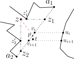
Figure 12: Illustrating a shortest path (the red dashed curve) from $z$ to $t$ crossing the interior of $\overline{v_{i}v_{i+1}}$ at $p$.

We extend a horizontal line segment from $v_{i}$ (resp., $v_{i+1}$) to the right until hitting the first point on $\partial\mathcal{Q}$, denoted by $u_{i}$ (resp., $u_{i+1}$); if $u_{i}$ and $u_{i+1}$ are not on the same elementary curve of $\mathcal{Q}$ (in which case one or both of $u_{i}$ and $u_{i+1}$ are extremes on different elementary curves), then we keep moving one or both of $u_{i}$ and $u_{i+1}$ horizontally to the right until hitting the next point on $\partial\mathcal{Q}$. By the definitions of $\mathcal{V}(\mathcal{Q})$ and $\mathcal{V}(g)$, in this way, we can always put both $u_{i}$ and $u_{i+1}$ on the same elementary curve of $\mathcal{Q}$, say $\beta$ (see Fig. 12); let $\beta(u_{i},u_{i+1})$ denote the portion of $\beta$ between $u_{i}$ and $u_{i+1}$. Let $R$ denote the region enclosed by $\overline{u_{i}v_{i}}$, $\overline{v_{i}v_{i+1}}$, $\overline{v_{i+1}u_{i+1}}$, and $\beta(u_{i},u_{i+1})$. Note that for any point $q\in R$, $q$ is horizontally visible to $\overline{v_{i}v_{i+1}}$ and thus is horizontally visible to $\overline{zz_{2}}$. In the following, we will show that $t$ must be in $R$, which proves the lemma.

Suppose to the contrary $t\not\in R$. We then show that the path $\pi(p,t)$ must intersect $\overline{v_{i}u_{i}}$ or $\overline{v_{i+1}u_{i+1}}$, which implies that there is a shortest $z$-$t$ path containing a point in $\{z_{1},z_{2}\}\cup\{\mathcal{V}(g)\cap\overline{z_{1}z_{2}}\}$, a contradiction (recall that we have an assumption that no shortest $s$-$t$ paths cross $\overline{a_{1}z_{1}}\cup\overline{a_{2}z_{2}}$). Indeed, if $\pi(p,t)$ intersects $\overline{v_{i}u_{i}}$ (resp., $\overline{v_{i+1}u_{i+1}}$), say, at a point $q$, then we can obtain a new $z$-$t$ path $\pi^{\prime}$ by replacing $\pi(z,q)$ with an $xy$-monotone path $\overline{zv_{i}}\cup\overline{v_{i}q}$ (resp., $\overline{zv_{i+1}}\cup\overline{v_{i+1}q}$), and $\pi^{\prime}$ is a shortest $z$-$t$ path containing a point in $\{z_{1},z_{2}\}\cup\{\mathcal{V}(g)\cap\overline{z_{1}z_{2}}\}$. Below, we show that $\pi(p,t)$ must intersect $\overline{v_{i}u_{i}}$ or $\overline{v_{i+1}u_{i+1}}$. Note that $\beta(u_{i},u_{i+1})$ may overlap with a gate of a canal. Depending on whether $\beta(u_{i},u_{i+1})$ overlaps with any canal gate, there are two possible cases.

1. If $\beta(u_{i},u_{i+1})$ does not overlap with any canal gate, then since $t\in\mathcal{M}$, $t\not\in R$, $p\in R$, and $\pi(p,t)\subseteq\mathcal{M}^{\prime}$, if we go from $t$ to $p$, we must enter $R$. The only place on the boundary of $R$ we can cross to enter $R$ is either $\overline{v_{i}u_{i}}$ or $\overline{v_{i+1}u_{i+1}}$. Hence, $\pi(t,p)$ must intersect $\overline{v_{i}u_{i}}$ or $\overline{v_{i+1}u_{i+1}}$.

2. If $\beta(u_{i},u_{i+1})$ overlaps with a canal gate, say $g_{1}$, then one may wonder that $\pi(t,p)$ could enter the interior of $R$ through $g_{1}$ without crossing any of $\overline{v_{i}u_{i}}$ and $\overline{v_{i+1}u_{i+1}}$. Since $g_{1}$ is a canal gate, one of $g_{1}$’s endpoints, say, $x$, must be a corridor path terminal, and $x$ may or may not be on $\beta(u_{i},u_{i+1})$. If $x$ is on $\beta(u_{i},u_{i+1})$, then since $x$ is in $\mathcal{V}(\mathcal{Q})$, $x$ cannot be in the interior of $\beta(u_{i},u_{i+1})$ and can only be at an endpoint of $\beta(u_{i},u_{i+1})$. Let $C$ be the canal that has $g_{1}$ as a gate, and $\pi(C)$ be the corridor path of $C$. If $\pi(t,p)$ enters the interior of $R$ through $g_{1}$, then it must travel through the canal $C$, implying that $\pi(t,p)\subseteq\mathcal{M}^{\prime}$ contains the corridor path $\pi(C)$. Since $x$ is on $\pi(C)$, $\pi(t,p)$ contains $x$. If $x$ is on $\beta(u_{i},u_{i+1})$ (and thus is an endpoint of $\beta(u_{i},u_{i+1})$), then $x$ is one of $u_{i}$ or $u_{i+1}$; hence, $\pi(t,p)$ intersects $\overline{v_{i}u_{i}}$ or $\overline{v_{i+1}u_{i+1}}$. Suppose now $x$ is not on $\beta(u_{i},u_{i+1})$. Then an endpoint of $\beta(u_{i},u_{i+1})$, say, $u_{i}$, lies on $g_{1}$ (but $u_{i}\not=x$). Further, $\pi(t,p)$ goes through $x$, and then enters $R$, but without intersecting any of $\overline{v_{i}u_{i}}$ and $\overline{v_{i+1}u_{i+1}}$. Thus, $\pi(t,p)$ must cross some point $q$ of $g_{1}$ to enter $R$. We can then replace the portion $\pi(x,q)$ of $\pi(t,p)$ by the segment $\overline{xq}\subseteq g_{1}$ to obtain a new shortest $t$-$p$ path. Since $u_{i}$ divides $g_{1}$ into two parts, one outside $R$ and containing $x$ and the other intersecting $R$ and containing $q$, the segment $\overline{xq}$ contains $u_{i}$. Hence, the new shortest $t$-$p$ path intersects $\overline{v_{i}u_{i}}$.

The lemma thus follows.

By Lemma 16, if the condition of the lemma holds, then we can always find a trivial shortest path from $z$ to $t$ by shooting vertical and horizontal rays from $z$ and $t$, respectively.

We have finished all possible cases for finding a shortest $s$-$t$ path when $s\in B$ and $t\in\mathcal{M}$. The next lemma is concerned with computing the special points $z_{1},z_{2}$, and $z$ for any point $s$ in $B$.

Lemma 17

With a preprocessing of $O(n_{B})$ time and space, the three special points $z_{1}$, $z_{2}$, and $z$ can be found in $O(\log n)$ time for any query point $s$ in $B$, where $n_{B}=|B|$.

Proof

Consider any query point $s\in B$. To determine $z_{1}$, $z_{2}$, and $z$, based on our previous discussions, it suffices to compute the two points $z_{1}^{\prime}$ and $z_{2}^{\prime}$. We only show how to design a data structure for computing $z_{1}^{\prime}$ since the solution for finding $z_{2}^{\prime}$ is similar. Note that $n_{B}\leq n$.

In the preprocessing, for each vertex $v$ of $B$, we find whether $v$ is horizontally visible to $g$, and if yes, mark $v$ as an h-vertex. All h-vertices of $B$ can be marked by computing the horizontal visibility of $B$ from $g$ in $O(n_{B})$ time [28, 32]. Also, in $O(n_{B})$ time, we compute the Euclidean shortest path tree $T_{1}$ from $a_{1}$ to all vertices of $B$ and the corresponding shortest path map $M_{1}$ in $B$ [20]; similarly, we compute the shortest path tree $T_{2}$ from $a_{2}$ and the corresponding shortest path map $M_{2}$.

For each vertex $v\in T_{1}$, we associate $v$ with two special vertices: $\alpha_{1}(v)$ and $\alpha_{2}(v)$, defined as follows. The vertex $\alpha_{1}(v)$ is the first h-vertex on the path in $T_{1}$ from $v$ to $a_{1}$ and $\alpha_{2}(v)$ is the child vertex of $\alpha_{1}(v)$ on the path in $T_{1}$ from $v$ to $a_{1}$; if $\alpha_{1}(v)=v$, then $\alpha_{2}(v)$ does not exist and we set $\alpha_{2}(v)=nil$. Note that $\alpha_{2}(v)$ is not an h-vertex if it exists. The $\alpha$ vertices for all vertices in $T_{1}$ can be computed in $O(n_{B})$ time by a depth-first search on $T_{1}$ starting at $a_{1}$. For each vertex $v\in T_{2}$, we compute only one special vertex for $v$, $\beta_{1}(v)$, which is the first h-vertex on the path in $T_{2}$ from $v$ to $a_{2}$. The $\beta$ vertices for all vertices of $T_{2}$ can also be computed in $O(n_{B})$ time.

This finishes our preprocessing, which takes $O(n_{B})$ time in total.

Below we find the point $z_{1}^{\prime}$ in $O(\log n)$ time. Let $\pi(s,a_{1})$ and $\pi(s,a_{2})$ be the Euclidean shortest paths in $B$ from $s$ to $a_{1}$ and $a_{2}$, respectively. For any point $p$, let $y(p)$ denote its $y$-coordinate.

By using the shortest path map $M_{1}$, we find the vertex, denoted by $v$, which directly connects to $s$ on $\pi(s,a_{1})$. Likewise, we find the vertex $u$ that directly connects to $s$ on $\pi(s,a_{2})$ using $M_{2}$. Both $v$ and $u$ are found in $O(\log n)$ time. Depending on whether $v=u$, there are two main cases.

1. If $v=u$, then clearly $s\neq z^{\prime}$. Let $v_{1}=\alpha_{1}(v)$ and $u_{1}=\beta_{1}(u)$. Note that $v_{1}$ and $u_{1}$ are available once we find $v$ and $u$. Depending on whether $v_{1}=u_{1}$, we further have two subcases.

   1. If $v_{1}=u_{1}$, then we claim $z^{\prime}=v_{1}=u_{1}$. Indeed, since $z^{\prime}$ is the last common vertex of $\pi(s,a_{1})$ and $\pi(s,a_{2})$ if we move on them from $s$, no vertex on $\pi(s,a_{1})\cap\pi(s,a_{2})$ can be horizontally visible to $g$ except possibly $z^{\prime}$. Because $v_{1}=u_{1}$, $v_{1}=u_{1}$ must be on $\pi(s,a_{1})\cap\pi(s,a_{2})$. Since $v_{1}=u_{1}$ is horizontally visible to $g$, $v_{1}=u_{1}=z^{\prime}$ must hold.

      By the definition of $z_{1}^{\prime}$, the above claim implies $z_{1}^{\prime}=z^{\prime}=u_{1}=v_{1}$.

   2. If $v_{1}\neq u_{1}$, then an easy observation is $y(v_{1})\geq y(u_{1})$. Let $v_{2}=\alpha_{2}(v)$. Note that due to $u=v$ and $v_{1}\neq u_{1}$, $\alpha_{2}(v)$ exists.

      If $y(v_{2})>y(v_{1})$, then the horizontal visibility of $v_{2}$ to $g$ is “blocked” by the path $\pi(v_{1},a_{1})$ (e.g., see Fig. 11(a)). Thus we obtain $z_{1}^{\prime}=v_{1}$.

      If $y(v_{2})\leq y(v_{1})$, then the horizontal visibility of $v_{2}$ to $g$ is “blocked” by the path $\pi(u_{1},a_{2})$ (e.g., see Fig. 11(b)). Thus we obtain that $z_{1}^{\prime}$ is the horizontal projection of $u_{1}$ on the line segment $\overline{v_{1}v_{2}}$, which can be computed in $O(1)$ time.

2. If $v\neq u$, then $s=z^{\prime}$. If $s$ is horizontally visible to $g$ (which can be determined in $O(\log n)$ time using the horizontal visibility decomposition of $B$), then $z_{1}^{\prime}=s=z^{\prime}$. Otherwise, let $v_{1}=\alpha_{1}(v)$ and $u_{1}=\beta_{1}(u)$. Depending on whether $v=v_{1}$, we further have two subcases.

   1. If $v\neq v_{1}$, then $\alpha_{2}(v)$ exists and we let $v_{2}=\alpha_{2}(v)$. Note that $\pi(s,a_{1})$ is a convex chain.

      Similar to the above discussion, if $y(v_{2})>y(v_{1})$, then we have $z_{1}^{\prime}=v_{1}$; otherwise, $z_{1}^{\prime}$ is the horizontal projection of $u_{1}$ on $\overline{v_{1}v_{2}}$.

   2. If $v=v_{1}$, then $s$ connects directly to $v_{1}$ on $\pi(s,a_{1})$. Similar to the above discussion, if $y(s)>y(v_{1})$, then we have $z_{1}^{\prime}=v_{1}$; otherwise, $z_{1}^{\prime}$ is the horizontal projection of $u_{1}$ on $\overline{v_{1}s}$.

Therefore, we can find the point $z_{1}^{\prime}$ in $O(\log n)$ time. The lemma thus follows.

We have discussed all possible cases of finding a shortest $s$-$t$ path when $s$ is in a bay $B$ and $t$ is in the ocean $\mathcal{M}$, and in each case, we can obtain a shortest path in $O(\log n)$ time.

4.3.3 The Point $t$ is in Another Bay

Let $B_{s}$ be the bay containing $s$ with gate $g_{s}$, and $B_{t}$ be the bay containing $t$ with gate $g_{t}$. In this case, any shortest $s$-$t$ path must cross both $g_{s}$ and $g_{t}$. The algorithm for this case is similar to the one for the case of $t\in\mathcal{M}$. Again, we need to consider different cases of how a shortest $s$-$t$ path may cross different portions of both the gates $g_{s}$ and $g_{t}$.

We define the points $z_{1}$, $z_{2}$, and $z$ in $B_{s}$ for $s$ in the same way as before, but denote them by $z_{1}(s)$, $z_{2}(s)$, and $z(s)$ instead. Similarly, we define the corresponding three points $z_{1}(t)$, $z_{2}(t)$, and $z(t)$ in $B_{t}$ for $t$. Based on our previous discussions, we have the following cases.

1. There is a shortest $s$-$t$ path containing a point $z_{s}$ in $\{z_{1}(s),z_{2}(s)\}$ and a point $z_{t}$ in $\{z_{1}(t),z_{2}(t)\}$. Note that both $z_{s}$ and $z_{t}$ are on their bay gates and thus are in $\mathcal{M}$.

   In this case, there must be a shortest $s$-$t$ path that is a concatenation of a shortest path $\pi(s,z_{s})$ from $s$ to $z_{s}$ in $B_{s}$, a shortest path $\pi(z_{s},z_{t})$ from $z_{s}$ to $z_{t}$ in $\mathcal{M}^{\prime}$, and a shortest path $\pi(z_{t},t)$ from $z_{t}$ to $t$ in $B_{t}$. The path $\pi(s,z_{s})$ can be found by using $\mathcal{D}(B_{s})$, i.e., the Euclidean two-point shortest path query data structure on $B_{s}$ [19], and similarly, $\pi(z_{t},t)$ can be found by using $\mathcal{D}(B_{t})$. The path $\pi(z_{s},z_{t})$ can be found by using our data structure for $\mathcal{M}^{\prime}$ in Lemma 8.

2. There is a shortest $s$-$t$ path that contains $z(s)$ and a point $z_{t}$ in $\{z_{1}(t),z_{2}(t)\}$.

   In this case, there must be a shortest $s$-$t$ path that is a concatenation of a shortest $s$-$z(s)$ path $\pi(s,z(s))$ in $B_{s}$, a shortest $z(s)$-$z_{t}$ path $\pi(z(s),z_{t})$, and a shortest $z_{t}$-$t$ path $\pi(z_{t},t)$ in $B_{t}$. The path $\pi(s,z(s))$ (resp., $\pi(z_{t},t)$) can be found by using $\mathcal{D}(B_{s})$ (resp., $\mathcal{D}(B_{t})$), and the path $\pi(z(s),z_{t})$ can be found by using similar algorithms as discussed above since $z_{t}$ is in $\mathcal{M}$.

3. There is a shortest $s$-$t$ path that contains $z(t)$ and a point $z_{s}$ in $\{z_{1}(s),z_{2}(s)\}$.

   This case is solved by using the similar approach as for Case 2 above.

4. There is a shortest $s$-$t$ path that contains $z(s)$ and $z(t)$.

   In this case, there must be a shortest $s$-$t$ path that is a concatenation of a shortest path $\pi(s,z(s))$ from $s$ to $z(s)$ in $B_{s}$, a shortest path $\pi(z(s),z(t))$ from $z(s)$ to $z(t)$, and a shortest path $\pi(z(t),t)$ from $z(t)$ to $t$ in $B_{t}$. The path $\pi(s,z(s))$ (resp., $\pi(z(t),t)$) can be found by using $\mathcal{D}(B_{s})$ (resp., $\mathcal{D}(B_{t})$). It remains to show how to compute $\pi(z(s),z(t))$ below.

Recall that we have defined a graph $G_{E}(g_{s})$ in $B_{s}$ on the points of $\mathcal{V}(g_{s})$, which consists of all points of $\mathcal{V}(\mathcal{Q})$ lying on $g_{s}$. We also find a gateway set $V_{g}(z(s),G_{E}(g_{s}))$ for $z(s)$ on $G_{E}(g_{s})$. Similarly, for $B_{t}$ and its gate $g_{t}$, we define $\mathcal{V}(g_{t})$, $G_{E}(g_{t})$, and $V_{g}(z(t),G_{E}(g_{t}))$. Let $G_{E}(\mathcal{M},g_{s},g_{t})$ be the graph formed by merging $G_{E}(\mathcal{M})$, $G_{E}(g_{s})$, and $G_{E}(g_{t})$. A shortest path from $z(s)$ to $z(t)$ can be found based on Lemmas 18 and 19 below, which are similar to Lemmas 14 and 16, respectively.

Lemma 18

If there is a shortest path from $z(s)$ to $z(t)$ containing a point in $\mathcal{V}(g_{s})\cap\overline{z_{1}(s)z_{2}(s)}$ and a point in $\mathcal{V}(g_{t})\cap\overline{z_{1}(t)z_{2}(t)}$, then there is a shortest path from $z(s)$ to $z(t)$ along $G_{E}(\mathcal{M},g_{s},g_{t})$ that contains a gateway of $z(s)$ in $V_{g}(z(s),G_{E}(g_{s}))$ and a gateway of $z(t)$ in $V_{g}(z(t),G_{E}(g_{t}))$.

Proof

Suppose there is a shortest $z(s)$-$z(t)$ path containing a point $p_{s}$ in $\mathcal{V}(g_{s})\cap\overline{z_{1}(s)z_{2}(s)}$ and a point $p_{t}$ in $\mathcal{V}(g_{t})\cap\overline{z_{1}(t)z_{2}(t)}$. Then by Lemma 13, there is a shortest $z(s)$-$p_{s}$ path $\pi(z(s),p_{s})$ along $G_{E}(g_{s})$ containing a gateway of $z(s)$ in $V_{g}(z(s),G_{E}(g_{s}))$ and there is a shortest $p_{t}$-$z(t)$ path $\pi(p_{t},z(t))$ along $G_{E}(g_{t})$ containing a gateway of $z(t)$ in $V_{g}(z(t),G_{E}(g_{t}))$. Since both $p_{s}$ and $p_{t}$ are in $\mathcal{V}(\mathcal{Q})$, by Lemma 4, there exists a shortest $p_{s}$-$p_{t}$ path $\pi(p_{s},p_{t})$ along $G_{E}(\mathcal{M})$.

The concatenation of $\pi(z(s),p_{s})$, $\pi(p_{s},p_{t})$, and $\pi(p_{t},z(t))$ is a shortest $z(s)$-$z(t)$ path, which is along the graph $G_{E}(\mathcal{M},g_{s},g_{t})$ and contains a gateway of $z(s)$ and a gateway of $z(t)$.

Lemma 19

If no shortest $z(s)$-$z(t)$ path contains any point of $\{z_{1}(s),z_{2}(s)\}\cup\{\mathcal{V}(g_{s})\cap\overline{z_{1}(s)z_{2}(s)}\}$, then $z(t)$ must be horizontally visible to $\overline{z(s)z_{2}(s)}$; similarly, if no shortest $z(s)$-$z(t)$ path contains any point of $\{z_{1}(t),z_{2}(t)\}\cup\{\mathcal{V}(g_{t})\cap\overline{z_{1}(t)z_{2}(t)}\}$, then $z(s)$ must be horizontally visible to $\overline{z(t)z_{2}(t)}$.

Proof

We prove only the case when no shortest $z(s)$-$z(t)$ path contains any point of $\{z_{1}(s),z_{2}(s)\}\cup\{\mathcal{V}(g_{s})\cap\overline{z_{1}(s)z_{2}(s)}\}$, $z(t)$ must be horizontally visible to $\overline{z(s)z_{2}(s)}$ (the other case is similar).

Let $\pi$ be a shortest $z(s)$-$z(t)$ path that intersects $g_{s}$ at a point $p_{s}$ and intersects $g_{t}$ at a point $p_{t}$ (see Fig. 13). Let $\pi(p_{1},p_{2})$ denote the subpath of $\pi$ between any two points $p_{1}$ and $p_{2}$ on $\pi$. We assume $\pi(z(s),p_{s})\subseteq B_{s}$, $\pi(p_{t},z(t))\subseteq B_{t}$, and $\pi(p_{s},p_{t})\subseteq\mathcal{M}^{\prime}$, since such a path $\pi$ always exists.

Let the points of $\mathcal{V}(g_{s})$ on $\overline{z_{1}(s)z_{2}(s)}$ be $v_{1},v_{2},\ldots,v_{m}$ ordered along $\overline{z_{1}(s)z_{2}(s)}$ from $z_{1}(s)$ to $z_{2}(s)$, and let $v_{0}=z_{1}(s)$ and $v_{m+1}=z_{2}(s)$. Suppose $p_{s}$ is in the interior of $\overline{v_{i}v_{i+1}}$, for some $i$ with $0\leq i\leq m$. We define $u_{i}$, $u_{i+1}$, $\beta(u_{i},u_{i+1})$, and $R$ in the same way as in the proof of Lemma 16.

Since $p_{t}$ is in $\mathcal{M}$, by the proof of Lemma 16, $p_{t}$ must be in the region $R$. Further, since $p_{t}$ is on $g_{t}\subseteq\partial\mathcal{Q}$, $p_{t}$ is on $\beta(u_{i},u_{i+1})$. Thus, $\beta(u_{i},u_{i+1})\cap g_{t}$ is not empty. Since $g_{t}$ is a line segment, $\beta(u_{i},u_{i+1})\cap g_{t}$ is also a line segment. Let $\overline{q_{1}q_{2}}=\beta(u_{i},u_{i+1})\cap g_{t}$. Thus, $p_{t}\in\overline{q_{1}q_{2}}$.

Recall that $z(t)$ is visible to $z_{1}(t)\in g_{t}$ and $\overline{z(t)z_{1}(t)}$ is horizontal. Hence, to prove that $z(t)$ is horizontally visible to $\overline{z(s)z_{2}(s)}$, it suffices to prove that $z_{1}(t)$ is horizontally visible to $\overline{z(s)z_{2}(s)}$. For this, it suffices to prove that $z_{1}(t)$ must be on $\overline{q_{1}q_{2}}$ since every point on $\overline{q_{1}q_{2}}\subseteq\beta(u_{i},u_{i+1})$ is horizontally visible to $\overline{z(s)z_{2}(s)}$. In the following, we prove $z_{1}(t)\in\overline{q_{1}q_{2}}$.

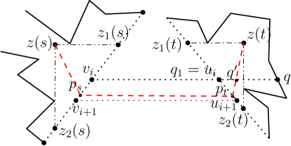
Figure 13: Illustrating a possible shortest path (the red dashed curve) from $z(s)$ to $z(t)$ crossing $\overline{u_{i}q}$. If this happens, we can find another shortest path $\pi(z(t),q^{\prime})\cup\overline{q^{\prime}v_{i}}\cup\overline{v_{i}z(s)}$, which contains $v_{i}$. In this example, $q_{1}=u_{i}$ and $q_{2}=u_{i+1}$.

Suppose to the contrary $z_{1}(t)\not\in\overline{q_{1}q_{2}}$ (see Fig. 13). Without loss of generality, we assume $q_{1}$ is closer to $z_{1}(t)$ than $q_{2}$. Since $p_{t}\in\overline{q_{1}q_{2}}$, $q_{1}\in\overline{p_{t}z_{1}(t)}\subseteq g_{t}$. This implies that $q_{1}$ is not an endpoint of $g_{t}$, and thus $q_{1}$ must be an endpoint of $\beta(u_{i},u_{i+1})$ (i.e., one of $u_{i}$ or $u_{i+1}$) since $\overline{q_{1}q_{2}}=\beta(u_{i},u_{i+1})\cap g_{t}$; assume $q_{1}=u_{i}$. We extend $\overline{v_{i}u_{i}}$ horizontally into the bay $B_{t}$ until hitting a point, say $q$, on the boundary of $B_{t}$ (see Fig. 13). The horizontal segment $\overline{u_{i}q}$ partitions $B_{t}$ into two sub-polygons such that $p_{t}$ and $z_{1}(t)$ are in different sub-polygons. Since $\overline{z(t)z_{1}(t)}$ is horizontal, $p_{t}$ and $z(t)$ are also in different sides of $\overline{u_{i}q}$, implying that the path $\pi(z(t),p_{t})$ must intersect $\overline{u_{i}q}$ since $\pi(z(t),p_{t})$ is in $B_{t}$. Let $q^{\prime}$ be the intersection of $\pi(z(t),p_{t})$ and $\overline{u_{i}q}$ (see Fig. 13). Then, the concatenation of $\pi(z(t),q^{\prime})$, $\overline{q^{\prime}v_{i}}$, and $\overline{v_{i}z(s)}$ is also a shortest path from $z(t)$ to $z(s)$ since $\overline{q^{\prime}v_{i}}\cup\overline{v_{i}z(s)}$ is $xy$-monotone. But this means that there is a shortest $z(s)$-$z(t)$ path containing $v_{i}$, contradicting with the lemma condition that no shortest $z(s)$-$z(t)$ path contains any point of $\{z_{1}(s),z_{2}(s)\}\cup\{\mathcal{V}(g_{s})\cap\overline{z_{1}(s)z_{2}(s)}\}$.

The above arguments prove that $z_{1}(t)$ is on $\overline{q_{1}q_{2}}$. The lemma thus follows.

By Lemmas 18 and 19, we can find a shortest $z(s)$-$z(t)$ path by either using the gateways of $z(s)$ and $z(t)$ in the merged graph $G_{E}(\mathcal{M},g_{s},g_{t})$ or shooting horizontal and vertical rays from $z(s)$ and $z(t)$. We have finished all possible cases for finding a shortest $s$-$t$ path when the two query points are in different bays. For each case, we compute a “candidate” shortest $s$-$t$ path, and take the one with the smallest length among all these cases (there are only a constant number of them).

It remains to solve the canal case, i.e., when the query points are in canals. The algorithm is similar to that for the bay case; the only difference is that we have to take care of two gates for each canal. Specifically, suppose $s$ is in a canal $C_{s}$ and $t$ is in a canal $C_{t}$. If $C_{s}\neq C_{t}$, then there must be a shortest $s$-$t$ path $\pi$ that intersects a gate of $C_{s}$ at a point $p_{s}$ and intersects a gate of $C_{t}$ at a point $p_{t}$ such that the subpath $\pi(s,p_{s})$ is in $C_{s}$, the subpath $\pi(p_{t},t)$ is in $C_{t}$, and the subpath $\pi(p_{s},p_{t})$ is in $\mathcal{M}^{\prime}$. Hence, we can use a similar approach as for the bay case to find a shortest $s$-$t$ path by considering all four gate pairs of $C_{s}$ and $C_{t}$. If $C_{s}=C_{t}$, while we can treat this case in the same way as for the case of $C_{s}\neq C_{t}$, we need to consider one more possible situation when a shortest $s$-$t$ path may be contained entirely in $C_{s}$, which is easy since $C_{s}$ is a simple polygon. If one of $C_{s}$ or $C_{t}$ is a bay, the case can be handled in a similar fashion.

We summarize the whole algorithm in the proof of the following theorem.

Theorem 4.1

We can build a data structure of size $O(n+h^{2}\log h4^{\sqrt{\log h}})$ in $O(n+h^{2}\log^{2}h4^{\sqrt{\log h}})$ time that can answer each two-point $L_{1}$ shortest path query in $O(\log n)$ time (i.e., for any two query points $s$ and $t$, the length of a shortest $s$-$t$ path can be found in $O(\log n)$ time and an actual path can be reported in additional time linear to the number of edges of the output path).

Proof

Our preprocessing algorithm consists of the following major steps.

1. Compute a triangulation of the free space $\mathcal{M}$ in $O(n+h\log^{1+\epsilon}h)$ time [2, 3]. Then produce all bays, canals, corridor paths, $\mathcal{M}$, and $\mathcal{V}(\mathcal{Q})$ in $O(n+h\log h)$ time [7, 8, 11].

2. Compute the vertical and horizontal visibility decompositions of $\mathcal{P}$ in $O(n+h\log^{1+\epsilon}h)$ time [2, 3]. Build a point location data structure [17, 31] for each of the two decompositions in $O(n)$ time, which is used for performing any vertical or horizontal ray-shooting in $O(\log n)$ time.

3. Construct the graph $G_{E}(\mathcal{M})$ of size $O(n+h\sqrt{\log h}2^{\sqrt{\log h}})$ in $O(n+h\log^{3/2}h2^{\sqrt{\log h}})$ time by Lemma 5.

4. Perform the preprocessing of Lemma 7 in $O(n+h\cdot\log^{3/2}h\cdot 2^{\sqrt{\log h}})$ time and $O(n+h\cdot\sqrt{\log h}\cdot 2^{\sqrt{\log h}})$ space.

5. Perform the preprocessing of Lemma 8 in $O(n+h^{2}\log^{2}h4^{\sqrt{\log h}})$ time and $O(n+h^{2}\log h4^{\sqrt{\log h}})$ space.

6. Compute a two-point Euclidean shortest path query data structure $\mathcal{D}(B)$ in each bay or canal $B$. Since the total number of vertices of all bays and canals is $O(n)$, this step takes $O(n)$ time.

7. Construct the graph $G_{E}(g)$ for the gate $g$ of every bay or canal by Lemma 12. The total space for all such graphs is $O(h\sqrt{\log h}2^{\sqrt{\log h}})$ and the total time for building all these graphs is $O(n+h\log^{3/2}h2^{\sqrt{\log h}})$, as proved below. First, each point of $\mathcal{V}(\mathcal{Q})$ can be on at most one bay or canal gate. Thus, the sum of $h_{g}$’s in Lemma 12 over all gates $g$ is $O(|\mathcal{V}(\mathcal{Q})|)$, which is $O(h)$. Second, the total number of obstacle vertices of all bays and canals is $O(n)$, and each canal has two gates. Hence, the sum of $n_{B}$’s in Lemma 12 over all bay and canals $B$ is $O(n)$.

8. Perform the preprocessing of Lemma 15 for the graphs $G_{E}(g)$ of all gates $g$, which can be done in totally $O(h\log^{3/2}h2^{\sqrt{\log h}})$ time and $O(h\sqrt{\log h}2^{\sqrt{\log h}})$ space.

9. Merge the graph $G_{E}(\mathcal{M})$ and the graphs $G_{E}(g)$ for all gates $g$ into a single graph $G_{E}(\mathcal{P})$, which takes $O(h)$ time since there are $O(h)$ points in $\mathcal{V}(\mathcal{Q})$. Thus, the size of $G_{E}(\mathcal{P})$ is $O(h\sqrt{\log h}2^{\sqrt{\log h}})$.

10. For each node $v$ of $G_{E}(\mathcal{P})$, compute a shortest path tree rooted at $v$ in $G_{E}(\mathcal{P})$. Maintain a shortest path length table such that for any two nodes $u$ and $v$ of $G_{E}(\mathcal{P})$, the length of a shortest path between $u$ and $v$ in $G_{E}(\mathcal{P})$ can be obtained in $O(1)$ time. This step takes $O(h^{2}\log h4^{\sqrt{\log h}})$ space and $O(h^{2}\log^{2}h4^{\sqrt{\log h}})$ time.

11. Perform the preprocessing of Lemma 17 for each bay and canal, which takes $O(n)$ space and $O(n)$ time in total.

In summary, the total preprocessing space and time are $O(n+h^{2}\log h4^{\sqrt{\log h}})$ and $O(n+h^{2}\log^{2}h4^{\sqrt{\log h}})$, respectively.

Consider any two query points $s$ and $t$. Next, we discuss our query algorithm that computes the length of a shortest $s$-$t$ path in $O(\log n)$ time and reports an actual path in additional time linear to the number of edges of the output path. We will not explicitly discuss how to report an actual path (which is similar to that in Lemma 8 and is easy).

First of all, as discussed in Section 2, we determine whether there exists a trivial shortest $s$-$t$ path by shooting horizontal and vertical rays from $s$ and $t$, which can be done in $O(\log n)$ time. In the following, we assume that there is no trivial shortest $s$-$t$ path. Depending on whether the query points are in the bays, canals, or the ocean $\mathcal{M}$, there are several possible cases.

Both query points are in $\mathcal{M}$.

In this case, we use the algorithm for Lemma 8 to find a shortest $s$-$t$ path in $O(\log n)$ time.

Only one query point is in $\mathcal{M}$.

Without loss of generality, we assume that $s$ is in a bay or a canal $B$ and $t$ is in $\mathcal{M}$. Further, we assume that $B$ is a canal since the case that $B$ is a bay can be considered as a special case.

Let $g^{1}$ and $g^{2}$ be the two gates of $B$. We define three points $z(s,g^{1})$, $z_{1}(s,g^{1})$, and $z_{2}(s,g^{1})$ for $s$ in $B$ with respect to the gate $g^{1}$ in the same way as we defined $z$, $z_{1}$, and $z_{2}$ before. Similarly, we define $z(s,g^{2})$, $z_{1}(s,g^{2})$, and $z_{2}(s,g^{2})$ for $s$ in $B$ with respect to the gate $g^{2}$. These points can be computed in $O(\log n)$ time by Lemma 17. Then, we compute the lengths of the following “candidate” shortest $s$-$t$ paths and return the one with the smallest length.

1. For each point $p\in\{z_{1}(s,g^{1}),z_{2}(s,g^{1}),z_{1}(s,g^{2}),z_{2}(s,g^{2})\}$, the path which is a concatenation of a shortest path $\pi(s,p)$ from $s$ to $p$ in $B$ and a shortest path $\pi(p,t)$ from $p$ to $t$ in $\mathcal{M}^{\prime}$.

   The path $\pi(s,p)$ can be found in $O(\log n)$ time by using the data structure $\mathcal{D}(B)$ on $B$, and the path $\pi(p,t)$ can be found in $O(\log n)$ time by Lemma 8.

2. For each point $p\in\{z(s,g^{1}),z(s,g^{2})\}$, the path which is a concatenation of a shortest path $\pi(s,p)$ from $s$ to $p$ in $B$ and a particular path $\pi(p,t)$ from $p$ to $t$.

   The path $\pi(s,p)$ can be found in $O(\log n)$ time by using the data structure $\mathcal{D}(B)$ on $B$. The path $\pi(p,t)$ is determined as follows. First, based on Lemma 16 (although $B$ is a bay in Lemma 16, the result also holds for canals because the lemma was proved with respect to a gate regardless of whether it is a gate of a bay or a canal), we check whether there exists a path from $p$ to $t$ consisting of only two line segments, by performing horizontal and vertical ray-shootings. If yes, then such a path is $\pi(p,t)$. Otherwise, by Lemmas 14 and 16, we find a shortest path from $p$ to $t$ along the merged graph $G_{E}(\mathcal{P})$ by using the gateways of $p$ and the gateways of $t$, which can be obtained in $O(\log n)$ time by Lemmas 15 and 7, respectively. Since both $p$ and $t$ have $O(\sqrt{\log h})$ gateways, a shortest $p$-$t$ path can be determined in $O(\log n)$ time using the gateway graph as discussed at the end of Section 3.

Neither query point is in $\mathcal{M}$.

Let $B_{s}$ be the bay or canal that contains $s$ and $B_{t}$ be the bay or canal that contains $t$.

If $B_{s}=B_{t}$ and $B_{s}$ is a bay, then by Lemma 9, we can find a shortest $s$-$t$ path by using the data structure $\mathcal{D}(B_{s})$ in $O(\log n)$ time.

Suppose $B_{s}\neq B_{t}$. Then we assume both $B_{s}$ and $B_{t}$ are canals since the other cases are just special cases of this case. Let $g^{1}_{s}$ and $g^{2}_{s}$ be the two gates of $B_{s}$ and $g^{1}_{t}$ and $g^{2}_{t}$ be the two gates of $B_{t}$. Similarly as before, we define the points $z(s,g_{s}^{i})$, $z_{1}(s,g_{s}^{i})$, and $z_{2}(s,g_{s}^{i})$ for $s$ with respect to $g_{s}^{i}$, and $z(t,g_{t}^{i})$, $z_{1}(t,g_{t}^{i})$, and $z_{2}(t,g_{t}^{i})$ for $t$ with respect to $g_{t}^{i}$, for $i=1,2$. These points can all be determined in $O(\log n)$ time by Lemma 17. Then we compute the lengths of the following “candidate” shortest $s$-$t$ paths and return the one with the smallest length.

1. For each pair of points $p_{s}$ and $p_{t}$ such that $p_{s}\in\{z_{1}(s,g_{s}^{1}),z_{2}(s,g_{s}^{1}),z_{1}(s,g_{s}^{2}),z_{2}(s,g_{s}^{2})\}$ and $p_{t}\in\{z_{1}(t,g_{t}^{1}),z_{2}(t,g_{t}^{1}),z_{1}(t,g_{t}^{2}),z_{2}(t,g_{t}^{2})\}$, the path which is a concatenation of a shortest path $\pi(s,p_{s})$ from $s$ to $p_{s}$ in $B_{s}$, a shortest path from $p_{s}$ to $p_{t}$ in $\mathcal{M}^{\prime}$, and a shortest path $\pi(p_{t},t)$ from $p_{t}$ to $t$ in $B_{t}$.

   The paths $\pi(s,p_{s})$ and $\pi(p_{t},t)$ can be found in $O(\log n)$ time by using $\mathcal{D}(B_{s})$ and $\mathcal{D}(B_{t})$, respectively. The path $\pi(p_{s},p_{t})$ can be obtained in $O(\log n)$ time by Lemma 8.

2. For each point $p_{s}\in\{z(s,g_{s}^{1}),z(s,g_{s}^{2})\}$ and each point $p_{t}\in\{z_{1}(t,g_{t}^{1}),z_{2}(t,g_{t}^{1}),z_{1}(t,g_{t}^{2}),z_{2}(t,g_{t}^{2})\}$, the path which is a concatenation of a shortest path from $s$ to $p_{s}$ in $B_{s}$, a particular path $\pi(p_{s},p_{t})$ from $p_{s}$ to $p_{t}$, and a shortest path from $p_{t}$ to $t$ in $B_{t}$.

   The paths $\pi(s,p_{s})$ and $\pi(p_{t},t)$ can be found in $O(\log n)$ time by using $\mathcal{D}(B_{s})$ and $\mathcal{D}(B_{t})$, respectively. Since $p_{t}$ is in $\mathcal{M}$, the particular path $\pi(p_{s},p_{t})$ is defined similarly as the path $\pi(p,t)$ in the second subcase of the above case when only one query point $t$ is in $\mathcal{M}$ and thus can be obtained by the similar approach.

3. For each point $p_{s}\in\{z_{1}(s,g_{s}^{1}),z_{2}(s,g_{s}^{1}),z_{1}(s,g_{s}^{2}),z_{2}(s,g_{s}^{2})\}$ and each point $p_{t}\in\{z(t,g_{t}^{1}),z(t,g_{t}^{2})\}$, the path which is a concatenation of a shortest path from $s$ to $p_{s}$ in $B_{s}$, a particular path $\pi(p_{s},p_{t})$ from $p_{s}$ to $p_{t}$, and a shortest path from $p_{t}$ to $t$ in $B_{t}$.

   This subcase is symmetric to the subcase immediately above and can be handled similarly.

4. For each point $p_{s}\in\{z(s,g_{s}^{1}),z(s,g_{s}^{2})\}$ and each point $p_{t}\in\{z(t,g_{t}^{1}),z(t,g_{t}^{2})\}$, the path which is a concatenation of a shortest path from $s$ to $p_{s}$ in $B_{s}$, a particular path $\pi(p_{s},p_{t})$ from $p_{s}$ to $p_{t}$, and a shortest path from $p_{t}$ to $t$ in $B_{t}$.

   The paths $\pi(s,p_{s})$ and $\pi(p_{t},t)$ can be found in $O(\log n)$ time by using $\mathcal{D}(B_{s})$ and $\mathcal{D}(B_{t})$, respectively. The particular path $\pi(p_{s},p_{t})$ is determined similarly as the path $\pi(p,t)$ in the second subcase of the above case when only one query point $t$ is in $\mathcal{M}$, but based on Lemmas 18 and 19 instead. Note that although $B_{s}$ and $B_{t}$ are bays in these lemmas, the results also hold for canals (actually, they are proved with respect to two gates regardless of whether they are gates of bays or canals). Specifically, we determine $\pi(p_{s},p_{t})$ as follows. Based on Lemma 19, we first check whether there exists a path from $p_{s}$ to $p_{t}$ consisting of only two line segments, by horizontal and vertical ray-shootings. If yes, then such a path is $\pi(p_{s},p_{t})$. Otherwise, by Lemmas 18 and 19, we find a shortest $p_{s}$-$p_{t}$ path along the merged graph $G_{E}(\mathcal{P})$ by using the gateways of $p_{s}$ and the gateways of $p_{t}$, which can be computed in $O(\log n)$ time by Lemma 15. Since both $p_{s}$ and $p_{t}$ have $O(\sqrt{\log h})$ gateways, a shortest $p_{s}$-$p_{t}$ path can be obtained in $O(\log n)$ time using the gateway graph as discussed in Section 3.

Finally, if $B_{s}=B_{t}$ and $B_{s}$ is a canal, then the algorithm is similar as for the above case with the difference that we must consider an additional “candidate” path that is a shortest $s$-$t$ path inside $B_{s}$, which can be found in $O(\log n)$ time by using the data structure $\mathcal{D}(B_{s})$.

Hence, in any case, we find a shortest $s$-$t$ path in $O(\log n)$ time. The theorem thus follows.

If we replace all enhanced graphs, e.g., $G_{E}(\mathcal{M})$ and $G_{E}(g)$ for every gate $g$, by the corresponding graphs similar to $G_{old}$ in [6] as discussed in Section 2, then we obtain the following results.

Corollary 3

We can build a data structure in $O(n+h^{2}\log^{2}h)$ time and space, such that each two-point shortest path query is answered in $O(\log n+\log^{2}h)$ time; alternatively, we can build a data structure in $O(nh\log h+h^{2}\log^{2}h)$ time and $O(nh\log h)$ space, such that each two-point shortest path query is answered in $O(\log n\log h)$ time.

Proof

If we replace all the enhanced graphs $G_{E}(\mathcal{M})$ and $G_{E}(g)$ for every gate $g$ of the bays and canals by the graphs similar to $G_{old}$ in [6] as discussed in Section 2, then the size of the new merged graph, denoted by $G_{old}(\mathcal{P})$, becomes $O(h\log h)$ instead of $O(h\sqrt{\log h}2^{\sqrt{\log h}})$. Hence, the data structure for Theorem 4.1 needs $O(n+h^{2}\log^{2}h)$ space and can be built in $O(n+h^{2}\log^{2}h)$ time by using the approach in [6]. However, using the new graph $G_{old}(\mathcal{P})$, each query for any two points in $\mathcal{M}$ can be answered in $O(\log^{2}h)$ time because there are $O(\log h)$ gateways for each query point. Therefore, any general two-point shortest path query can be answered in $O(\log^{2}h+\log n)$ time, by using a similar query algorithm as in Theorem 4.1. We omit the details.

In the result above, we compute a shortest path tree rooted at each node in the merged graph $G_{old}(\mathcal{P})$. Alternatively, we can compute a shortest path map in the free space $\mathcal{F}$ for each node $v$ of $G_{old}(\mathcal{P})$, such that given any query point $t$, the length of a shortest path from $v$ to $t$ can be found in $O(\log n)$ time and an actual path can be reported in additional time linear to the number of edges of the output path. Each such shortest path map is of size $O(n)$ and can be computed in $O(n+h\log h)$ time [7, 8, 11] (after the free space $\mathcal{F}$ is triangulated). Since the size of $G_{old}(\mathcal{P})$ is $O(h\log h)$, the overall preprocessing time and space are $O(nh\log h+h^{2}\log^{2}h)$ and $O(nh\log h)$, respectively. For querying, since a query point may have $O(\log h)$ gateways and for each gateway $v$, we can determine the shortest path from $v$ to the other query point in $O(\log n)$ time, the total query time is $O(\log h\log n)$. We omit the details.

5 The Weighted Rectilinear Case

In this section, we extend our techniques in Section 3 to the weighted rectilinear case. In the weighted rectilinear case, every polygonal obstacle $P\in\mathcal{P}$ is rectilinear and weighted, i.e., each edge of $P$ is either horizontal or vertical and $P$ has a weight $w(P)\geq 0$ ($w(P)=+\infty$ is possible). If a line segment $e$ is in $P$, then the weighted length of $e$ is $x\cdot(1+w(P))$, where $x$ is the $L_{1}$ length of $e$. Any polygonal path $\pi$ can be divided into a sequence of maximal line segments such that each segment is contained in the same obstacle or in the free space $\mathcal{F}$; the weighted length of $\pi$ is the sum of the weighted lengths of all maximal line segments of $\pi$.

Consider a vertex $v$ of any rectilinear obstacle $P$ such that the interior angle of $P$ at $v$ is $3\pi/2$. We define the internal projections of $v$ on the boundary $\partial P$ of $P$ as follows. Suppose $\overline{u_{1}v}$ and $\overline{u_{2}v}$ are the two edges of $P$ incident to $v$. We extend $\overline{u_{1}v}$ into the interior of $P$ along the direction from $u_{1}$ to $v$ until we hit $\partial P$ at the first point, which is an internal projection of $v$; similarly, we define another interval projection of $v$ by extending $\overline{u_{2}v}$. Internal projections are used to control shortest paths that pass through the interior of obstacles.

The “visibility” in the weighted case is defined in a slightly different way: Two points $p$ and $q$ are visible to each other if $\overline{pq}$ is entirely in either $\mathcal{F}$ or an obstacle.

Let $\mathcal{V}$ be the set of all obstacle vertices of $\mathcal{P}$, their internal projections, and all type-1 Steiner points. Then $|\mathcal{V}|=O(n)$. We build a graph $G_{E}(\mathcal{V})$ on $\mathcal{V}$ similar to the one presented in Section 3, with the following differences. (1) The visibility here is based on the new definition above. (2) Since a path can travel through the interior of any obstacle, for each cut-line $l$, an edge in $G_{E}(\mathcal{V})$ connects every two consecutive Steiner points on $l$, whose weight is the weighted length of the line segment connecting the two points. (3) In addition to the vertical cut-lines, there are also horizontal cut-lines, which are defined similarly and have type-2 and type-3 Steiner points defined on them similarly to those on the vertical cut-lines. Thus, $G_{E}(\mathcal{V})$ has $O(n\sqrt{\log n}2^{\sqrt{\log n}})$ nodes and edges.

Lemma 20

The graph of $G_{E}(\mathcal{V})$ can be built in $O(n\log^{3/2}n2^{\sqrt{\log n}})$ time.

Proof

We obtain all internal projections of $\mathcal{V}$ by computing the horizontal and vertical visibility decompositions of every obstacle in $\mathcal{P}$. We find the four projection points on $\partial\mathcal{P}$ (i.e., $p^{r},p^{l},p^{u}$, and $p^{d}$) for all obstacle vertices $p$ of $\mathcal{P}$ in $O(n\log n)$ time by computing the horizontal and vertical visibility decompositions of $\mathcal{F}$. These can be all done in totally $O(n\log n)$ time.

Then we compute the vertical and horizontal cut-line trees, which takes $O(n\log n)$ time since $|\mathcal{V}|=O(n)$. Next, we compute the Steiner points and the graph edges. Below, we only show how to compute those related to the vertical cut-lines; those related to the horizontal cut-lines can be computed in a similar way. Let $T^{v}(\mathcal{V})$ denote the vertical cut-line tree.

As in Lemma 1, we can compute the type-2 and type-3 Steiner points on all cut-lines of $T^{v}(\mathcal{V})$ by traversing $T^{v}(\mathcal{V})$ in a top-down manner. Since the internal projections and $\{p^{r},p^{l},p^{u},p^{d}\}$ for each obstacle vertex $p$ have been obtained, we can compute all $O(n\sqrt{\log n}2^{\sqrt{\log n}})$ such Steiner points in $O(n\sqrt{\log n}2^{\sqrt{\log n}})$ time; the corresponding horizontal graph edges connecting these Steiner points and the points of $\mathcal{V}$ can also be computed.

It remains to compute the graph edges connecting every pair of consecutive Steiner points on each cut-line of $T^{v}(\mathcal{V})$, which takes $O(n\log^{3/2}n2^{\sqrt{\log n}})$ time by a plane sweeping algorithm, as follows. We first sort all Steiner points on each cut-line. We then sweep a vertical line $L$ from left to right and use a balanced binary search tree $T$ to maintain the intervals between the obstacle edges of $\mathcal{P}$ intersecting $L$. By standard techniques, we augment $T$ to also maintain the weighted length information along $L$ such that for any two points $p$ and $q$ on $L$, the weighted length of $\overline{pq}$ can be obtained in $O(\log n)$ time using $T$. During the sweeping, when $L$ encounters a cut-line $l$, for every two consecutive Steiner points $p$ and $q$ on $l$, we use $T$ to determine in $O(\log n)$ time the weighted length of the edge connecting $p$ and $q$. Since there are $O(n\sqrt{\log n}2^{\sqrt{\log n}})$ pairs of consecutive Steiner points on all cut-lines, it takes $O(n\log^{3/2}n2^{\sqrt{\log n}})$ time to compute all these graph edges.

Hence, we can build the graph $G_{E}(\mathcal{V})$ in $O(n\log^{3/2}n2^{\sqrt{\log n}})$ time.

Consider any two query points $s$ and $t$. For simplicity of discussion, we assume that both $s$ and $t$ are in $\mathcal{F}$ (the general case can also be handled similarly). With a preprocessing of $O(n^{2})$ time and space, a shortest $s$-$t$ path that does not contain any vertex of $\mathcal{V}$ can be found in $O(\log n)$ time [6]. Thus in the following, we focus on finding a shortest $s$-$t$ path containing at lease one vertex of $\mathcal{V}$.

Let $Y(s)$ be the set of $s$ and the four projections of $s$ on $\partial\mathcal{P}$, i.e., $Y(s)=\{s,s^{l},s^{r},s^{u},s^{d}\}$; similarly, let $Y(t)=\{t,t^{l},t^{r},t^{u},t^{d}\}$. It was shown in [6] that it suffices to find a shortest path from $p$ to $q$ containing a vertex of $\mathcal{V}$ for every $p\in Y(s)$ and every $q\in Y(t)$. With a little abuse of notation, we let $s$ be any point in $Y(s)$ and $t$ be any point in $Y(t)$. Our goal is to find a shortest $s$-$t$ path that contains at lease one vertex of $\mathcal{V}$. Unless otherwise indicated, any shortest $s$-$t$ path mentioned below refers to a shortest $s$-$t$ path that contains a vertex of $\mathcal{V}$.

In [6], similar to the discussions in Section 2, $O(\log n)$ gateways for $s$ and $O(\log n)$ gateways for $t$ were defined, such that any shortest $s$-$t$ path must contain a gateway of $s$ and a gateway of $t$. Hence by using the gateway graph, a shortest $s$-$t$ path can be found in $O(\log^{2}n)$ time.

Based on our enhanced graph $G_{E}(\mathcal{V})$, as in Section 3, we define a new gateway set $V_{g}(s,G_{E}(\mathcal{V}))$ of size $O(\sqrt{\log n})$ for $s$ and a new gateway set $V_{g}(t,G_{E}(\mathcal{V}))$ of size $O(\sqrt{\log n})$ for $t$. The gateway set $V_{g}(s,G_{E}(\mathcal{V}))$ contains $O(\sqrt{\log n})$ Steiner points on the vertical cut-lines defined in the same way as those in $V^{2}_{g}(s,G_{E})$ in Section 3; similarly, $V_{g}(s,G_{E}(\mathcal{V}))$ also contains $O(\sqrt{\log n})$ Steiner points on the horizontal cut-lines. The gateway set $V_{g}(t,G_{E}(\mathcal{V}))$ is defined similarly. Using a similar proof as for Lemma 2, we can show that there exists a shortest $s$-$t$ path containing a gateway of $s$ in $V_{g}(s,G_{E}(\mathcal{V}))$ and a gateway of $t$ in $V_{g}(t,G_{E}(\mathcal{V}))$. Next, we show how to compute the two gateway sets and (the weights of) their gateway edges. Below, we discuss only the case for $s$.

The fractional cascading approach [4] used in Section 3 can still compute the gateway set $V_{g}(s,G_{E}(\mathcal{V}))$ in $O(\log n)$ time, but it cannot compute the weights of the gateway edges in $O(\log n)$ time for the following reasons. Consider a gateway $v\in V_{g}(s,G_{E}(\mathcal{V}))$, say on a vertical cut-line $l$. Then there is a gateway edge $(s,v)$ that consists of two line segments $\overline{ss_{h}(l)}$ and $\overline{s_{h}(l)v}$ (recall that $s_{h}(l)$ is the horizontal projection of $s$ on $l$). Hence, the weighted length of the edge $(s,v)$ is the sum of the weighted lengths of these two line segments. It was shown in [6] that $\overline{ss_{h}(l)}$ must be in the free space (since $s$ is in $\mathcal{F}$); thus, the weighted length of $\overline{ss_{h}(l)}$ is easy to compute. However, the vertical segment $\overline{s_{h}(l)v}$ may intersect multiple obstacles [6]. We give an algorithm to compute in $O(\log n)$ time the gateways and the weights of the gateway edges for $s$ in the next lemma.

Lemma 21

With a preprocessing of $O(n^{2}\log n)$ time and $O(n^{2})$ space, the gateways of $V_{g}(s,G_{E}(\mathcal{V}))$ for $s$ and their weighted edges can be computed in $O(\log n)$ time.

Proof

We discuss only how to compute the gateways of $V_{g}(s,G_{E}(\mathcal{V}))$ that are on the vertical cut-lines since those on the horizontal cut-lines can be computed similarly. Further, for simplicity of discussion, we only compute the gateways of $V_{g}(s,G_{E}(\mathcal{V}))$ above $s$ (i.e., above the horizontal line through $s$) since those below $s$ can be computed similarly. Below, with a little abuse of notation, we let $V_{g}(s,G_{E}(\mathcal{V}))$ refer to the set of its gateways on the vertical cut-lines and above $s$.

We follow the terminology in Section 3. Recall that $s$ has $O(\log n)$ projection cut-lines in the vertical cut-line tree $T^{v}(\mathcal{V})$. Let $S_{l}$ be the set of all projection cut-lines of $s$ in $T^{v}(\mathcal{V})$. For each projection cut-line $l\in S_{l}$, let $v(l)$ be the Steiner point on $l$ immediately above the horizontal projection $s_{h}(l)$ of $s$ on $l$. Let $S_{v}=\{v(l)\ |\ l\in S_{l}\}$. By their definitions, $V_{g}(s,G_{E}(\mathcal{V}))$ is a subset of $S_{v}$ (since each gateway of $V_{g}(s,G_{E}(\mathcal{V}))$ is on a relevant projection cut-line of $s$ in $T^{v}(\mathcal{V})$). Hence, to compute $V_{g}(s,G_{E}(\mathcal{V}))$ and their gateway edges, it suffices to compute the set $S_{v}$ and the weighted lengths of $\overline{ss_{h}(l)}\cup\overline{s_{h}(l)v(l)}$ for all projection cut-lines $l\in S_{l}$. Since $\overline{ss_{h}(l)}$ is in $\mathcal{F}$ for any projection cut-line $l$ of $s$ [6] (because $s\in\mathcal{F}$), it suffices to compute the weighted length of $\overline{s_{h}(l)v(l)}$. Below, for any line segment $\overline{ab}$, let $d_{w}(\overline{ab})$ denote the weighted length of $\overline{ab}$. Let $S_{w}=\{\overline{s_{h}(l)v(l)}\ |\ l\in S_{l}\}$.

We use fractional cascading [4] to obtain $S_{v}$ in $O(\log n)$ time, with a similar approach as for Lemma 3. To compute the weighted lengths of the segments in $S_{w}$, we need to build another fractional cascading data structure in the preprocessing.

For every cut-line $l$ of $T^{v}(\mathcal{V})$, we compute the intersections of $l$ with all obstacle edges of $\mathcal{P}$; let $I(l)$ be the set of such intersections. Clearly, $|I(l)|=O(n)$. We sort these intersections and the Steiner points on $l$ to obtain a sorted list $I^{\prime}(l)$. For all $n$ cut-lines of $T^{v}(\mathcal{V})$, this takes totally $O(n^{2}\log n)$ time, because the total number of Steiner points is $O(n\sqrt{\log n}2^{\sqrt{\log n}})$ (which is $O(n^{2})$) and the total number of intersections between the cut-lines and the obstacle edges is $O(n^{2})$.

Consider the sorted set $I^{\prime}(l)$ for any cut-line $l$ of $T^{v}(\mathcal{V})$. For any two consecutive points $p_{1}$ and $p_{2}$ in $I^{\prime}(l)$, the entire segment $\overline{p_{1}p_{2}}$ is either in $\mathcal{F}$ or in the same obstacle. From top to bottom in $I^{\prime}(l)$, for each point $p\in I^{\prime}(l)$, we compute the weighted length $d_{w}(\overline{pp^{*}})$ and associate it with $p$, where $p^{*}$ is the highest point in $I^{\prime}(l)$. Further, for each point $p\in I^{\prime}(l)$, we maintain a weight $w_{p}$, defined as follows: Suppose $p^{\prime}$ is the point in $I^{\prime}(l)$ immediately below $p$; if the interior of $\overline{pp^{\prime}}$ is contained in an obstacle, then $w_{p}$ is the weight of that obstacle, and $w_{p}=0$ otherwise. Since $I^{\prime}(l)$ is sorted, computing such information in $I^{\prime}(l)$ takes $O(|I^{\prime}(l)|)$ time. With such information, for any query point $q$ on $l$, suppose $p$ is the point in $I^{\prime}(l)$ that is immediately above $q$; then we have $d_{w}(\overline{qp^{*}})=d_{w}(\overline{pp^{*}})+(1+w_{p})\cdot d_{w}(\overline{pq})$. Hence, once we know the point $p$ for $q$, $d_{w}(\overline{qp^{*}})$ can be computed in $O(1)$ time; further, for any point $p^{\prime}$ in $I^{\prime}(l)$ above $q$, we have $d_{w}(\overline{qp^{\prime}})=d_{w}(\overline{qp^{*}})-d_{w}(\overline{p^{\prime}p^{*}})$, which is computed in $O(1)$ time since the value $d_{w}(\overline{p^{\prime}p^{*}})$ is already stored at $p^{\prime}$.

In the preprocessing, we build another fractional cascading data structure on $T^{v}(\mathcal{V})$ and the sorted lists $I^{\prime}(l)$ for all cut-lines $l$ of $T^{v}(\mathcal{V})$, which takes $O(n^{2})$ space and $O(n^{2}\log n)$ time.

For any query point $s$, we first use a similar approach as for Lemma 3 to compute the set $S_{v}$ in $O(\log n)$ time. For each projection cut-line $l\in S_{l}$, let $v^{\prime}(l)$ be the point in $I^{\prime}(l)$ immediately above $s_{h}(l)$. Note that $v^{\prime}(l)$ is between $v(l)$ and $s_{h}(l)$. We can use the above fractional cascading data structure to compute the points $v^{\prime}(l)$ for all $l\in S_{l}$ in $O(\log n)$ time (since the cut-lines of $S_{l}$ are at the nodes of a path from the root to a leaf in $T^{v}(\mathcal{V})$). Then for each $l\in S_{l}$, to compute $d_{w}(\overline{s_{h}(l)v(l)})$, as discussed above, we have $d_{w}(\overline{s_{h}(l)v(l)})=d_{w}(\overline{s_{h}(l)p^{*}})-d_{w}(\overline{v(l)p^{*}})$, where $p^{*}$ is the highest point in $I^{\prime}(l)$ and $d_{w}(\overline{s_{h}(l)p^{*}})=d_{w}(\overline{v^{\prime}(l)p^{*}})+(1+w_{v^{\prime}(l)})\cdot d_{w}(\overline{s_{h}(l)v^{\prime}(l)})$. Since both $v(l)$ and $v^{\prime}(l)$ have been computed, $d_{w}(\overline{s_{h}(l)v(l)})$ is obtained in $O(1)$ time. Hence, the weighted lengths of all segments in $S_{w}$ are computed in $O(\log n)$ time.

The lemma thus follows.

The following theorem summarizes our algorithm for the weighted rectilinear case.

Theorem 5.1

For the weighted rectilinear case, we can build a data structure of size $O(n^{2}\log n4^{\sqrt{\log n}})$ in $O(n^{2}\log^{2}n4^{\sqrt{\log n}})$ time that can answer each query in $O(\log n)$ time (i.e., for any two query points $s$ and $t$, the weighted length of a shortest $s$-$t$ path can be found in $O(\log n)$ time and an actual path can be reported in additional time linear to the number of edges of the output path).

Proof

In the preprocessing, we compute the graph $G_{E}(\mathcal{V})$ by Lemma 20. For each node $v$ of $G_{E}(\mathcal{V})$, we compute a shortest path tree rooted at $v$ in $G_{E}(\mathcal{V})$. We maintain a shortest path length table such that for any two nodes $u$ and $v$ in $G_{E}(\mathcal{V})$, the (weighted) length of the shortest path from $u$ to $v$ in $G_{E}(\mathcal{V})$ is obtained in $O(1)$ time. Computing all shortest path trees in $G_{E}(\mathcal{V})$ takes $O(n^{2}\log n4^{\sqrt{\log n}})$ space and $O(n^{2}\log^{2}n4^{\sqrt{\log n}})$ time. We also perform the preprocessing for Lemma 21. Hence, the preprocessing takes $O(n^{2}\log n4^{\sqrt{\log n}})$ space and $O(n^{2}\log^{2}n4^{\sqrt{\log n}})$ time in total.

Consider any two query points $s$ and $t$. First, we use the approach in [6] to find a shortest $s$-$t$ path that does not contain any obstacle vertex of $\mathcal{P}$ (if any), after a preprocessing of $O(n^{2})$ time and space. Below, we focus on finding a shortest $s$-$t$ path containing an obstacle vertex of $\mathcal{P}$, which must contain a gateway of $s$ in $V_{g}(s,G_{E}(\mathcal{V}))$ and a gateway of $t$ in $V_{g}(t,G_{E}(\mathcal{V}))$. By Lemma 21, we can compute both $V_{g}(s,G_{E}(\mathcal{V}))$ and $V_{g}(t,G_{E}(\mathcal{V}))$ in $O(\log n)$ time. Then, a shortest $s$-$t$ path can be found by building a gateway graph (as discussed in Section 3) in $O(\log n)$ time since the sizes of both $V_{g}(s,G_{E}(\mathcal{V}))$ and $V_{g}(t,G_{E}(\mathcal{V}))$ are $O(\sqrt{\log n})$. As in [6], after the shortest $s$-$t$ path length is computed, an actual shortest $s$-$t$ path can be reported by using the shortest path trees of the nodes in $G_{E}(\mathcal{V})$, in time linear to the number of edges of the output path.

The theorem thus follows.

References

- [1] S.W. Bae and Y. Okamato. Querying two boundary points for shortest paths in a polygonal domain. Computational Geometry: Theory and Applications, 45:284–293, 2012.
- [2] R. Bar-Yehuda and B. Chazelle. Triangulating disjoint Jordan chains. International Journal of Computational Geometry and Applications, 4(4):475–481, 1994.
- [3] B. Chazelle. Triangulating a simple polygon in linear time. Discrete and Computational Geometry, 6:485–524, 1991.
- [4] B. Chazelle and L. Guibas. Fractional cascading: I. A data structuring technique. Algorithmica, 1(1):133–162, 1986.
- [5] D.Z. Chen, J. Hershberger, and H. Wang. Computing shortest paths amid convex pseudodisks. SIAM Journal on Computing, 42(3):1158–1184, 2013.
- [6] D.Z. Chen, K.S. Klenk, and H.-Y.T. Tu. Shortest path queries among weighted obstacles in the rectilinear plane. SIAM Journal on Computing, 29(4):1223–1246, 2000.
- [7] D.Z. Chen and H. Wang. A nearly optimal algorithm for finding shortest paths among polygonal obstacles in the plane. In Proc. of the 19th European Symposium on Algorithms (ESA), pages 481–492, 2011.
- [8] D.Z. Chen and H. Wang. Computing shortest paths among polygonal obstacles in the plane. arXiv:1202.5715v1, 2012.
- [9] D.Z. Chen and H. Wang. Computing the visibility polygon of an island in a polygonal domain. In Proc. of the 39th International Colloquium on Automata, Languages and Programming (ICALP), pages 218–229, 2012.
- [10] D.Z. Chen and H. Wang. Computing shortest paths among curved obstacles in the plane. In Proc. of the 29th ACM Symposium on Computational Geometry (SoCG), pages 369–378, 2013.
- [11] D.Z. Chen and H. Wang. shortest path queries among polygonal obstacles in the plane. In Proc. of 30th Symposium on Theoretical Aspects of Computer Science (STACS), pages 293–304, 2013.
- [12] D.Z. Chen and H. Wang. Visibility and ray shooting queries in polygonal domains. In Proc. of the 13rd International Symposium on Algorithms and Data Structures (WADS), pages 369–378, 2013.
- [13] L.P. Chew. Planning the shortest path for a disc in time. In Proc. of the 1st Annual ACM Symposium on Computational Geometry (SoCG), pages 214–220, 1985.
- [14] Y.-J. Chiang and J.S.B. Mitchell. Two-point Euclidean shortest path queries in the plane. In Proc. of the Annual ACM-SIAM Symposium on Discrete Algorithms (SODA), pages 215–224, 1999.
- [15] K. Clarkson, S. Kapoor, and P. Vaidya. Rectilinear shortest paths through polygonal obstacles in time. In Proc. of the 3rd Annual Symposium on Computational Geometry (SoCG), pages 251–257, 1987.
- [16] K. Clarkson, S. Kapoor, and P. Vaidya. Rectilinear shortest paths through polygonal obstacles in time. Manuscript, 1988.
- [17] H. Edelsbrunner, L. Guibas, and J. Stolfi. Optimal point location in a monotone subdivision. SIAM Journal on Computing, 15(2):317–340, 1986.
- [18] H.A. ElGindy and P. Mitra. Orthogonal shortest route queries among axis parallel rectangular obstacles. International Journal of Computational Geometry and Application, 4:3–24, 1994.
- [19] L.J. Guibas and J. Hershberger. Optimal shortest path queries in a simple polygon. Journal of Computer and System Sciences, 39(2):126–152, 1989.
- [20] L.J. Guibas, J. Hershberger, D. Leven, M. Sharir, and R.E. Tarjan. Linear-time algorithms for visibility and shortest path problems inside triangulated simple polygons. Algorithmica, 2(1-4):209–233, 1987.
- [21] J. Hershberger. A new data structure for shortest path queries in a simple polygon. Information Processing Letters, 38(5):231–235, 1991.
- [22] J. Hershberger and L. Guibas. An shortest path algorithm for a non-rotating convex body. Journal of Algorithms, 9(1):18–46, 1988.
- [23] J. Hershberger and J. Snoeyink. Computing minimum length paths of a given homotopy class. Computational Geometry: Theory and Applications, 4(2):63–97, 1994.
- [24] J. Hershberger and S. Suri. An optimal algorithm for Euclidean shortest paths in the plane. SIAM Journal on Computing, 28(6):2215–2256, 1999.
- [25] J. Hershberger, S. Suri, and H. Yıldız. A near-optimal algorithm for shortest paths among curved obstacles in the plane. In Proc. of the 29th Annual Symposium on Computational Geometry (SoCG), pages 359–368, 2013.
- [26] R. Inkulu and S. Kapoor. Planar rectilinear shortest path computation using corridors. Computational Geometry: Theory and Applications, 42(9):873–884, 2009.
- [27] R. Inkulu, S. Kapoor, and S.N. Maheshwari. A near optimal algorithm for finding Euclidean shortest path in polygonal domain. In arXiv:1011.6481v1, 2010.
- [28] B. Joe and R.B. Simpson. Corrections to Lee’s visibility polygon algorithm. BIT, 27:458–473, 1987.
- [29] S. Kapoor and S.N. Maheshwari. Efficient algorithms for Euclidean shortest path and visibility problems with polygonal obstacles. In Proc. of 4th Annual ACM Symposium on Computational Geometry (SoCG), pages 172–182, 1988.
- [30] S. Kapoor, S.N. Maheshwari, and J.S.B. Mitchell. An efficient algorithm for Euclidean shortest paths among polygonal obstacles in the plane. Discrete and Computational Geometry, 18(4):377–383, 1997.
- [31] D. Kirkpatrick. Optimal search in planar subdivisions. SIAM Journal on Computing, 12(1):28–35, 1983.
- [32] D.T. Lee. Visibility of a simple polygon. Computer Vision, Graphics, and Image Processing, 22(2):1983, 207–221.
- [33] D.T. Lee and F.P. Preparata. Euclidean shortest paths in the presence of rectilinear barriers. Networks, 14(3):393–410, 1984.
- [34] D.T. Lee, C.D. Yang, and T.H. Chen. Shortest rectilinear paths among weighted obstacles. International Journal of Computational Geometry and Applications, 1(2):109–124, 1991.
- [35] J.S.B. Mitchell. An optimal algorithm for shortest rectilinear paths among obstacles. Abstracts of the 1st Canadian Conference on Computational Geometry (CCCG), 1989.
- [36] J.S.B. Mitchell. A new algorithm for shortest paths among obstacles in the plane. Annals of Mathematics and Artificial Intelligence, 3(1):83–105, 1991.
- [37] J.S.B. Mitchell. shortest paths among polygonal obstacles in the plane. Algorithmica, 8(1):55–88, 1992.
- [38] J.S.B. Mitchell. Shortest paths among obstacles in the plane. International Journal of Computational Geometry and Applications, 6(3):309–332, 1996.
- [39] J.S.B. Mitchell. Geometric shortest paths and network optimization, in Handbook of Computational Geometry, J.-R Sack and J. Urrutia (eds.), pages 633–702. Elsevier, Amsterdam, the Netherlands, 2000.
- [40] J.S.B. Mitchell and C.H. Papadimitriou. The weighted region problem: Finding shortest paths through a weighted planar subdivision. Journal of the ACM, 38:18–73, 1991.