Magnetic reconnection in a comparison of topology and helicities in two and three dimensional resistive MHD simulations

Abstract

Through a direct comparison between numerical simulations in two and three dimensions, we investigate topological effects in reconnection. A simple estimate on increase in reconnection rate in three dimensions by a factor of $\sqrt{2}$, when compared with a two-dimensional case, is confirmed in our simulations. We also show that both the reconnection rate and the fraction of magnetic energy in the simulations depend linearly on the height of the reconnection region. The degree of structural complexity of a magnetic field and the underlying flow is measured by current helicity and cross-helicity. We compare results in simulations with different computational box heights.

I Introduction

Reconnection of a magnetic field is a process in which magnetic field lines change connection with respect to their sources. In effect, magnetic energy is converted into kinetic and thermal energies, which accelerate and heat the plasma. Historically, reconnection was first observed in the solar flares and the Earth’s magnetosphere, but today it is also investigated in star formation theory and astrophysical dynamo theory. Recently, reconnection has also been invoked in the acceleration of cosmic rays [9].

In solar flares, oppositely directed magnetic flux is first accumulated, and then reconnection occurs, enabling energy transfer to kinetic energy and heating of plasma. From such an ejection of matter, we can observe the onset of reconnection and estimate the energy released in this process. Recent results from measurements by the instruments onboard the Solar Dynamic Observatory [21] have revealed new unexpected features and show that even the morphology of the solar reconnection is still not completely understood.

In the context of accretion disks around protostars, neutron stars and black holes, reconnection is a part of the transport of heat, matter and angular momentum. It enables re-arrangement of the magnetic field, after which angular momentum can be transported from the matter that is infalling from an accretion disk, towards the central object. In Čemeljić et al. [6] we performed resistive simulations of star-disk magnetospheric outflows in 2D axisymmetric simulations. On-going reconnection is producing a fast, light micro-ejections of matter from the close vicinity of a disk gap. When going to three-dimensional simulations, more precise model of reconnection is needed, as it will define the topology of magnetic field. In the cases where flows are less ordered, turbulent reconnection has been invoked [10].

The Sweet-Parker model [22] was the first proposed model for reconnection. Parker [14] solved time-independent, non-ideal MHD equations for two regions of plasma with oppositely directed magnetic fields pushed together. Particles are accelerated by a pressure gradient, with use of the known facts about magnetic field diffusion. Viscosity and compressibility are assumed to be unimportant, so that the magnetic field energy converts completely into heat. This model is robust, but gives too slow a time for the duration of reconnection, when compared with observed data for solar flares. Petschek [17] proposed another model, for fast reconnection. For energy conversion, he added stationary slow-mode shocks between the inflow and outflow regions. This decreased the aspect ratio of the diffusion region to the order of unity, and increased the energy release rate, so that the observed data were now better matched. However, his model fails in the explanation of solar flares because fast reconnection can persist only for a very short time period. Many aspects of the reconnection process have been studied since, but the problem of the speed of reconnection remains unsolved.

Because of numerical difficulties, research on reconnection was for a few decades constrained to two-dimensional solutions. In three dimensional space there are more ways of reconnection than in two dimensions, and the very nature of reconnection is different [19]. There is still no full assessment of three dimensional reconnection – for a recent review, see Pontin [18].

Our 2D setup here is a familiar Harris current sheet, an exact stationary solution to the problem of a current sheet separating regions of oppositely directed magnetic field in a fully ionized plasma [7]. It is possible to obtain a Petschek-like reconnection in resistive-MHD simulations with uniform resistivity, but it demands special care with the setup of boundary conditions, as described in [3]. To avoid this issue, we chose to set a spatially asymmetric profile for resistivity, as suggested in [3]. In 3D simulations, we build a column of matter above such a Harris 2D configuration, with resistivity dependent on height in the third direction. Because of a modification of the resulting shocks, it enables a Petchek reconnection also in the third dimension.

We first investigate differences between the reconnection rate in 2D and 3D numerical simulations, by comparing energies in the computational box. Then we compare change of current helicity and cross-helicity with the increasing height of the matter column in the third direction.

II Numerical setup for simulations of reconnection

Magnetic reconnection is considered in the magnetohydrodynamic approximation (MHD) in our simulations. There are other possibilities. An entirely different approach, with kinetic reconnection, is described in [5] and references therein. Such reconnection is a consequence of the instability of thin current sheets in a self-consistent consideration about ion and electron inertia, and dissipative wave-particle resonances.

Ideal MHD, which is the study of the dynamics of a perfectly conducting fluid, is not appropriate for the description of reconnection. This is because a fluid must cross the field lines of magnetic field, not follow them, as required by ideal MHD. This means that for numerical simulations with reconnection, a non-ideal resistive MHD is needed. For our simulations we use the pluto (v. 4.0) code [11] in the parallel option. The equations we solve are, in Gaussian cgs units:

$$\frac{\partial\rho}{\partial t}+\nabla\cdot(\rho\mathchoice{\mbox{\boldmath$\displaystyle V$}}{\mbox{\boldmath$\textstyle V$}}{\mbox{\boldmath$\scriptstyle V$}}{\mbox{\boldmath$\scriptscriptstyle V$}})=0$$ (1)

$$\rho\left[\frac{\partial\mathchoice{\mbox{\boldmath$\displaystyle V$}}{\mbox{\boldmath$\textstyle V$}}{\mbox{\boldmath$\scriptstyle V$}}{\mbox{\boldmath$\scriptscriptstyle V$}}}{\partial t}+\left(\mathchoice{\mbox{\boldmath$\displaystyle V$}}{\mbox{\boldmath$\textstyle V$}}{\mbox{\boldmath$\scriptstyle V$}}{\mbox{\boldmath$\scriptscriptstyle V$}}\cdot\nabla\right)\mathchoice{\mbox{\boldmath$\displaystyle V$}}{\mbox{\boldmath$\textstyle V$}}{\mbox{\boldmath$\scriptstyle V$}}{\mbox{\boldmath$\scriptscriptstyle V$}}\right]+\nabla p-\frac{\mathchoice{\mbox{\boldmath$\displaystyle j$}}{\mbox{\boldmath$\textstyle j$}}{\mbox{\boldmath$\scriptstyle j$}}{\mbox{\boldmath$\scriptscriptstyle j$}}\times\mathchoice{\mbox{\boldmath$\displaystyle B$}}{\mbox{\boldmath$\textstyle B$}}{\mbox{\boldmath$\scriptstyle B$}}{\mbox{\boldmath$\scriptscriptstyle B$}}}{c}=0$$ (2)

$$\frac{\partial\mathchoice{\mbox{\boldmath$\displaystyle B$}}{\mbox{\boldmath$\textstyle B$}}{\mbox{\boldmath$\scriptstyle B$}}{\mbox{\boldmath$\scriptscriptstyle B$}}}{\partial t}-\nabla\times\left(\mathchoice{\mbox{\boldmath$\displaystyle V$}}{\mbox{\boldmath$\textstyle V$}}{\mbox{\boldmath$\scriptstyle V$}}{\mbox{\boldmath$\scriptscriptstyle V$}}\times\mathchoice{\mbox{\boldmath$\displaystyle B$}}{\mbox{\boldmath$\textstyle B$}}{\mbox{\boldmath$\scriptstyle B$}}{\mbox{\boldmath$\scriptscriptstyle B$}}-\frac{4\pi}{c}\eta\mathchoice{\mbox{\boldmath$\displaystyle j$}}{\mbox{\boldmath$\textstyle j$}}{\mbox{\boldmath$\scriptstyle j$}}{\mbox{\boldmath$\scriptscriptstyle j$}}\right)=0\,,\nabla\cdot\mathchoice{\mbox{\boldmath$\displaystyle B$}}{\mbox{\boldmath$\textstyle B$}}{\mbox{\boldmath$\scriptstyle B$}}{\mbox{\boldmath$\scriptscriptstyle B$}}=0$$ (3)

$$\rho\left[{\frac{\partial e}{\partial t}}+\left(\mathchoice{\mbox{\boldmath$\displaystyle V$}}{\mbox{\boldmath$\textstyle V$}}{\mbox{\boldmath$\scriptstyle V$}}{\mbox{\boldmath$\scriptscriptstyle V$}}\cdot\nabla\right)e\right]+p(\nabla\cdot\mathchoice{\mbox{\boldmath$\displaystyle V$}}{\mbox{\boldmath$\textstyle V$}}{\mbox{\boldmath$\scriptstyle V$}}{\mbox{\boldmath$\scriptscriptstyle V$}})-\frac{4\pi}{c^{2}}\eta\mathchoice{\mbox{\boldmath$\displaystyle j$}}{\mbox{\boldmath$\textstyle j$}}{\mbox{\boldmath$\scriptstyle j$}}{\mbox{\boldmath$\scriptscriptstyle j$}}^{2}=0\,,$$ (4)

with $\rho$ and p for the density and pressure, and V and B for the velocity and magnetic field. The electric current density is given by Ampère’s law $\mathchoice{\mbox{\boldmath$\displaystyle j$}}{\mbox{\boldmath$\textstyle j$}}{\mbox{\boldmath$\scriptstyle j$}}{\mbox{\boldmath$\scriptscriptstyle j$}}=c\nabla\times\mathchoice{\mbox{\boldmath$\displaystyle B$}}{\mbox{\boldmath$\textstyle B$}}{\mbox{\boldmath$\scriptstyle B$}}{\mbox{\boldmath$\scriptscriptstyle B$}}/{4\pi}$. The internal energy (per unit mass) is $e=p/(\rho(\gamma-1))$, where $\gamma$ is the effective polytropic index. We work in the adiabatic regime, with $\gamma=5/3$, so that the ideal gas law is $\rho=\gamma p/c_{s}^{2}$, where $c_{s}$ is the sound speed and $\eta$ is the electrical resistivity. Here we do not consider the influence of terms other than Ohmic resistivity.

Our simulations are set in a uniform Cartesian grid with $X\times Y\times Z$ = $(200\times 400\times 100)$ grid cells = $([-1,1]\times[-2,2]\times[0,1])$ in code units. The same resolution, equal in all three directions, is kept in simulations with different heights and in the 2D simulations. The number of cells in the Z direction is changed so as to obtain the same resolution with each height of the box. Our results are compared to [4] as a reference. There, a nonuniform grid is used, with the smallest grid spacing 7 times smaller in X, and 3 times smaller in the Y direction, than in our uniform spacing. We performed simulations with different resolutions, and found the number of cells for which the reconnection occurred and qualitatively resembled the reference. In the results with finer resolution, only the time needed to reach different stages varied. With coarser resolution, reconnection did not occur, as the current sheet was not enough resolved.

II.1 Initial and boundary conditions

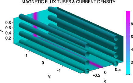
Figure 1: Setup of initial and boundary conditions in our simulations in three dimensions. In two dimensional simulations, Z=0. Color grading is showing a current density in code units, at the boundary planes; the diameter of the magnetic flux tube is set proportional to the magnetic field strength. We start with a 2D simulation in Cartesian coordinates $X\times Y$. Increasing the height of a box in Z direction, we compare the reconnection rates and other interesting quantities in the flow.

To ease a comparison of results, we choose the same initial conditions for density, pressure, velocity and two regions of oppositely directed magnetic field as in [4]. The so called Harris current sheet is formed initially with magnetic field $\mathbf{B_{2}}(x)=\mathbf{y}B_{0}\tanh({\mathbf{x}}/b)$, which is parallel to the Y axis and is varying in the X direction. The amplitude of the magnetic field is chosen to be $B_{0}=1$, and the initial half-width of the current sheet is $b=0.1$. We set the plasma $\beta=0.35$, the initial pressure to $p(x)=1.25-B_{2}^{2}/2$, and the density $\rho(x)=2p(x)/\beta$. To obtain Petschek reconnection with spatially uniform resistivity, boundary conditions need to be overspecified at one of the inflow boundaries by imposing the mass density, two components of the velocity, one component of the magnetic field, and the total energy [3]. To avoid such issues, we include the anomalous Ohmic resistivity (which is for a few orders of magnitude larger than microscopic resistivity), with a profile asymmetric in the X-Y plane and dependent on height in the Z-direction:

$$\eta=(\eta_{0}-\eta_{1})\exp{[-(x/a_{1})^{2}-(y/a_{2})^{2}]}$$ (5)

$$+(\eta_{0}-\eta_{1})\exp{-(x/a_{1})^{2}-(z/a_{3})^{2}}+\eta_{1}$$

$$=\eta_{1}+(\eta_{0}-\eta_{1})\exp{[-(x/a_{1})^{2}]}$$

$$\cdot(\exp{[-(y/a_{2})^{2}]}+\exp{[-(z/a_{2})^{2}]})\ ,$$

with the characteristic lengths of the resistivity variation in each direction $a_{1}$=0.05, and $a_{2}$=$a_{3}$=0.02. Constant factors in the resistivity $\eta_{0}=10^{-3}$ and $\eta_{1}=3\times 10^{-5}$ are also equal to those in [4], for easier comparison. We checked that $\eta_{1}$ is above the order of numerical resistivity at a given resolution. The level of numerical resistivity we found by a direct comparison of simulations with different minimum resistivity; it is of the order of $10^{-6}$. All our simulations have been performed with the value of the resistivity set above the numerical resistivity. The resistivity is then set equal to $\eta$ for $y\geq 0$, or to $\eta_{0}$ for $y<0$. At all the boundaries, we impose the free (“outflow”) boundary conditions, extrapolating the flow from the box in the ghost zones.

In the pluto code setup we used Cartesian coordinates, ideal equation of state, and the “dimensional splitting” option, which uses Strang operator splitting to solve the equations in the multi-dimension case. The spatial order of integration was set as “linear”, meaning that a piecewise TVD linear interpolation is applied, accurate to second order in space. We used the second order in time Runge Kutta evolution scheme RK2, with the Eight-Waves option for constraining the $\nabla\cdot\mathchoice{\mbox{\boldmath$\displaystyle B$}}{\mbox{\boldmath$\textstyle B$}}{\mbox{\boldmath$\scriptstyle B$}}{\mbox{\boldmath$\scriptscriptstyle B$}}=0$ at the truncation level. As the approximate Riemann solver, we use the Lax-Friedrichs scheme (“tvdlf” solver option in pluto).

We first present the well known results in 2D, to introduce a concept of reconnection and measurement of the reconnection rate.

III Results in 2D

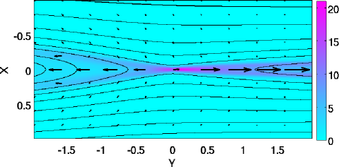
Figure 2: Reconnection in two dimensions at T=30 in code units, with current density shown in color grading, magnetic field contour lines in solid lines, and arrows showing velocity.

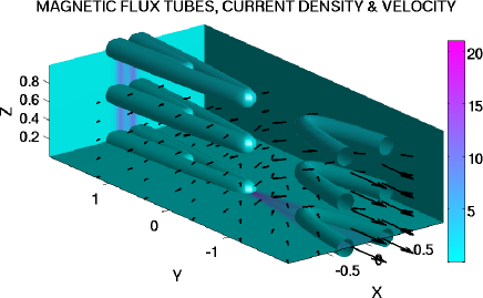
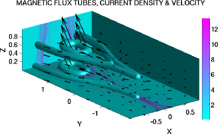
Figure 3: Solutions in 3D in the first case, without the asymmetry in resistivity in the Z direction at T=30 (Left panel), and in the second case, with the asymmetry in the Z direction at T=70 (Right panel). Color grading is showing the toroidal current density at the boundary planes; tubes show a choice of the magnetic flux tubes, with the diameter of the tube set proportional to the magnetic field strength; arrows show velocity. A change in connectivity of the magnetic flux tubes in 3D, triggered by the asymmetry in resistivity in the vertical plane, additionally changes, and complicates, the topology of magnetic field.

Reconnection in 2D is an extensively investigated topic, but still with inconclusive results. It is not even clear if the approach with numerical simulations in MHD correctly describes onset of reconnection, especially in models which invoke turbulence. Here we assume that MHD simulations can provide correct rates.

Reconnection rate in the two-dimensional case can be estimated in the different ways, depending on the dominating physical properties in the system. The first such estimate was given by Parker [14, 15], with the Alfvén Mach number $M_{\mathrm{SP}}=V_{\mathrm{i}}/V_{\mathrm{A}}=S^{-1/2}$. The Lundquist number $S=\tau_{Ohm}/\tau_{adv}=LV_{\mathrm{A}}/\eta$ is the ratio of the advective over the resistive term in the Equation (3). In an astrophysical case, the length scale is so large that the obtained reconnection rate is way too small, when compared to the observed reconnection events on the Sun or in the Earth’s magnetosphere.

To improve the model, Petschek [17] assumed that the plasma can also be accelerated by slow shocks. Then the reconnection rate is $M_{\mathrm{P}}=\pi/(8\ln S)$. For the current sheet in a small region, the Petschek model gives orders of magnitude faster reconnection than the Sweet-Parker model, up to 0.1. The reason is that in the Petschek model the reconnection rate is not strongly dependent on the Lundquist number. For the current sheet extending to the whole reconnection area, both models give the same reconnection rate.

The reconnection rate can also be estimated from the turbulent motions [10]. For the case of only Ohmic resistivity, we can estimate the distance to which a magnetic field can diffuse in time $\tau_{D}$ as $\ell\sim(\eta\tau_{D})^{1/2}$. This means that two lines can merge only if their distance is of the order of $\Delta=\ell/\sqrt{S}$. In combination with mass conservation, one obtains the reconnection rate $M_{\mathrm{SP}}$.

In our 2D simulation, initial conditions are the same as in Baty et al. [4], with asymmetric resistivity. We did not specify fixed conditions at the inflow boundary in the X direction. Instead, our boundary conditions are left open to “outflow”, so that a steady state will not be reached. The density nearby the box boundaries along the Y direction does not change until T=70 in code units, confining the matter inside the box. Starting from time T=1, a Petschek reconnection is obtained. In the case shown in Figure 2, the reconnection rate is of the order of $M_{\mathrm{P}}=0.1$. The Figure shows a resulting velocity structure with current density and magnetic field during reconnection, at T=30. After T=100, because of reflections back into the computational box, and matter leaving the box, the results become unsuitable for comparison with steady state solutions.

IV Results in 3D

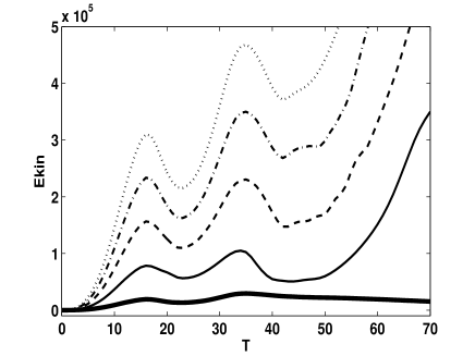
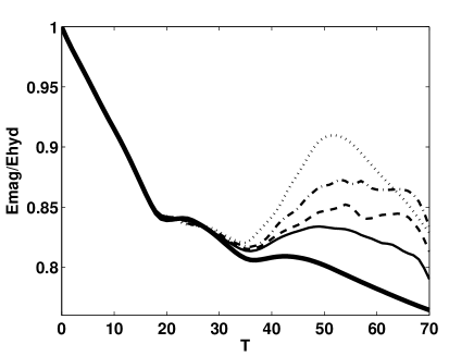
Figure 4: Time dependence of the energy with different heights of the computational box in our simulations with reconnection in all three directions. In the Left panel is shown the kinetic energy, and in the Right panel is shown the ratio of magnetic to the sum of internal and kinetic energy. Results with different heights of the box h=1, 2, 3 and 4, are shown in solid, dashed, dot-dashed and dotted lines, respectively. In thick solid line is shown the result with height h=0.25 in the case with reconnection only in the X-Y plane, which is our reference 2D case. Kinetic energy during the build-up of reconnection is linearly increasing with height of the computational box, with the factor of proportionality about 2. The fraction of magnetic energy is steadily decreasing with time, until the reconnection in the third direction starts; then it increases proportionally with height.

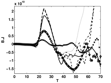
Figure 5: Time evolution of current helicity in $X\leq 0$ half of the computational box. Results with different heights of the box h=0.25, 0.5, 1, 2, 3 and 4, are shown in black cross and diamond marked, solid, dashed, dot-dashed and dotted lines, respectively.

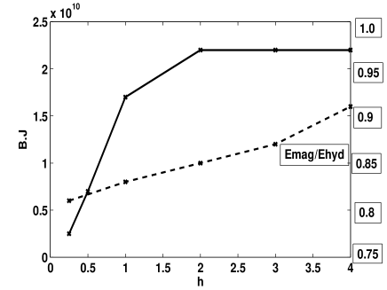
Figure 6: In solid line is shown maximum variation in current helicity with height of the computational box, during the increase in reconnection. Values are taken from results at T=23, shown in Figure 5. In dashed line is shown the maximum variation of fraction of magnetic energy in dependence of h, taken from results about T=50 shown in Figure 4. Note the different scales in the vertical axes of the plot; the right side axis denotes the fraction of magnetic energy.

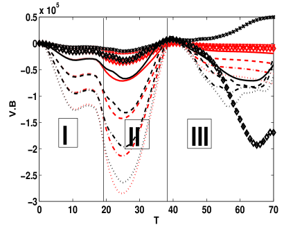
Figure 7: Time evolution of cross helicity in $X\leq 0$ half of the computational box. Lines have the same meaning as in Figure 5. Results in the first case, with reconnection only in the X-Y plane, are shown in red lines, with the same line style coding. Three time intervals mark time of build-up of reconnection in the X-Y plane (I), increase in reconnection in the Z-direction (II), and short increase in the fraction of magnetic energy, during the re-organization of the magnetic field because of reconnection (III).

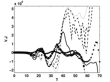
Figure 8: Time evolution of “mixed helicity” in $X\leq 0$ half of the computational box. Lines have the same meaning as in Figure 5.

When we set up the 3D simulation with the same asymmetry in resistivity as in the 2D case, and add the dependence of the resistivity with Z, we obtain in each X-Y parallel plane results similar to the 2D case, as shown in Figure 3. This is because of the current sheet at X=0 along the Y-Z plane. Without some perturbation, which would break the stability of this current sheet, a flow does not really have three, but still only two degrees of freedom, as if the 2D simulations would be stacked atop each other. Instead of introducing the perturbation – as has been done for example in simulations with Hall resistivity by Huba & Rudakov [8] – we rather introduce the dependence of resistivity with height (the Z direction) in our prescription of resistivity, in the same way as we did in the X-Y plane. For small heights of the box, the result still resembles the 2D result. With increase in height, shocks are modified in the Z-direction, so that at each height, the shock is of different density. This enables the Petschek reconnection in the Y-Z plane, which is expelling matter in the Z-direction. In Figure 3 both reconnection in the X-Y and Y-Z plane are visible.

In Priest & Schrijver [20] it has been estimated that one additional degree of freedom results in an increase by a factor of the order of $\sqrt{2}$ in the reconnection rate. To estimate the reconnection rate in 3D, we compute the energy in the computational box. For the Lundquist number S, from the Sweet-Parker reconnection rate it follows that $V_{\mathrm{i,3D}}^{2}/V_{\mathrm{i,2D}}^{2}=E_{\mathrm{k,3D}}/E_{\mathrm{k,2D}}=2$. This means that if in 3D simulations the reconnection rate increases for $\sqrt{2}$, compared to the 2D simulation, the corresponding kinetic energy increases by a factor of 2. We can now verify if this estimate is true.

The results for time dependence of the integral kinetic energy for the different heights of the box are shown in Figure 4. As in the 2D case, we compare results during the phase of the simulation when reconnection rate increases, and boundaries still do not change much from the initial conditions. We find agreement with the above prediction: that kinetic energy in a 3D simulation is about double the energy in 2D, for the same length scale. We also find that the trend continues linearly with increase in height of the box. After the peak in reconnection (about T=50 in our simulations with reconnection in both the X-Y and Y-Z planes), as was the case in 2D simulations, reflections back into the computational box and matter leaving the box make results for different heights incomparable. With less density, matter leaves the box with higher velocity, and the kinetic energy increases. For maintaining the stationary reconnection rate, driving at the boundaries would be needed. Here we do not investigate such a case.

In Aly [1, 2] it is argued that the maximum magnetic energy the force-free system can store, is in the configuration without loops in the magnetic field. Any loop would, when straightened, lead to an “open field” of larger energy. Our simulations are not in the force-free regime, but measurement of the dependence of this ratio with decrease in height of the computational box could still be informative. Our result is shown in Figure 4. The fraction of magnetic energy in total energy increases linearly with the increase in box height.

A general measure of reconnection should anticipate not only well ordered, but also complex reconnection, for example in the case of reconnection in turbulent fluids. A change in topology of magnetic field can to some degree be measured by a “knottedness of tangled vortex lines” [12]. For any vector field $\textstyle F$, the quantity $\mathchoice{\mbox{\boldmath$\displaystyle F$}}{\mbox{\boldmath$\textstyle F$}}{\mbox{\boldmath$\scriptstyle F$}}{\mbox{\boldmath$\scriptscriptstyle F$}}\cdot(\nabla\times\mathchoice{\mbox{\boldmath$\displaystyle F$}}{\mbox{\boldmath$\textstyle F$}}{\mbox{\boldmath$\scriptstyle F$}}{\mbox{\boldmath$\scriptscriptstyle F$}})$ is called the helicity density. The integral over a closed volume is then the helicity. For a vector field which is invariant to the change from a right-hand to left-hand orientation of the coordinates, helicity is zero [13]. One such example are our simulations here, which have a mirror symmetry across the Y-Z plane at X=0. To obtain non-zero results, we always integrate only over half of the computational box, in the interval ($-0.5\leq x\leq 0$). In a non-symmetric case, this integral should be taken across the whole computational box.

We compute three quantities related to helicity, to measure the degree of complexity of the velocity and magnetic field: current helicity H_c and cross-helicity H_VB

$$H_{\mathrm{c}}=\int\mathchoice{\mbox{\boldmath$\displaystyle B$}}{\mbox{\boldmath$\textstyle B$}}{\mbox{\boldmath$\scriptstyle B$}}{\mbox{\boldmath$\scriptscriptstyle B$}}\cdot(\nabla\times\mathchoice{\mbox{\boldmath$\displaystyle B$}}{\mbox{\boldmath$\textstyle B$}}{\mbox{\boldmath$\scriptstyle B$}}{\mbox{\boldmath$\scriptscriptstyle B$}})dV,\ H_{\mathrm{VB}}=\int\mathchoice{\mbox{\boldmath$\displaystyle V$}}{\mbox{\boldmath$\textstyle V$}}{\mbox{\boldmath$\scriptstyle V$}}{\mbox{\boldmath$\scriptscriptstyle V$}}\cdot\mathchoice{\mbox{\boldmath$\displaystyle B$}}{\mbox{\boldmath$\textstyle B$}}{\mbox{\boldmath$\scriptstyle B$}}{\mbox{\boldmath$\scriptscriptstyle B$}}dV\ ,$$ (6)

for which results are shown in Figures 5 and 7, and a quantity H_VJ which we provisionally call “mixed helicity”

$$H_{\mathrm{VJ}}=\int\mathchoice{\mbox{\boldmath$\displaystyle V$}}{\mbox{\boldmath$\textstyle V$}}{\mbox{\boldmath$\scriptstyle V$}}{\mbox{\boldmath$\scriptscriptstyle V$}}\cdot\mathchoice{\mbox{\boldmath$\displaystyle J$}}{\mbox{\boldmath$\textstyle J$}}{\mbox{\boldmath$\scriptstyle J$}}{\mbox{\boldmath$\scriptscriptstyle J$}}dV,$$ (7)

shown in Figure 8. Integrations are always performed over half of the computational box.

There are three separate time intervals, marked in Figure 7, which are present in all the results: (I) build-up of reconnection in the X-Y plane, (II) increase in reconnection in the Z-direction, and (III) short increase in the fraction of magnetic energy, during the re-organization of the magnetic field because of reconnection.

Increase in current helicity with height of the computational box during the interval II is shown in Figure 6, together with the change in energy. For more than double height of the box, increase in H_c is small during the interval II. Only during the interval III, when reconnection in the third direction is fully established, current helicity increases. Cross helicity is better describing the three dimensional reconnection, as it increases linearly with height of the box for the full 3D reconnection, with h$\geq 1$. For smaller heights, h=0.25 and 0.5, reconnection in the Z direction does not follow the trend – this could be an artifact of our setup, with directional asymmetry in resistivity. Cross helicity, shown in Figure 7 is also clearly showing difference between reconnection in 2D and in 3D throughout both intervals II and III.

“Mixed helicity”, shown in Figure 8 shows there is more structure to fields of velocity and current in all the intervals from I-III, than revealed in the other two helicities or energies. It remains to be seen, in simulations with less ordered, or turbulent reconnection, how much of this structure is related to strictly directional asymmetry in our setup of resistivity.

V Summary

We have presented new results with the direct comparison of numerical simulations of reconnection in two and three dimensions. Reconnection in our simulations is facilitated by an asymmetry in the Ohmic resistivity. Without asymmetry, reconnection does not occur in our setup. Asymmetry in the X-Y plane is enabling the reconnection in that plane, and dependence of the resistivity with height in Z-direction is changing the shocks in the Z-direction, so that the Petschek reconnection starts also in the Y-Z plane.

By comparing the integral kinetic energy in 2D and 3D computations, we find that the 3D simulation proceeds with a reconnection rate which is for a factor $\sqrt{2}$ larger from the rate in the 2D simulation. This finding confirms the simple analytic estimate from Priest & Schrijver [20]. We also show that a fraction of magnetic energy in total energy is increasing linearly with the increase in box height.

We obtained our results in the case when reconnection was set by an asymmetry in resistivity. There are other means of facilitating reconnection. One natural generalization from a 2D simulation of X-point collapse of a magnetic field into a localized current layer in a 3D situation is to obtain points in space at which the magnetic field strength is zero – 3D null points. Topology of such points is characterized by a pair of field lines forming a separatrix surface, which separates portions of magnetic field which are of different topologies. Yet another way to form a current sheet in 3D is to connect two such null points – forming a separator line ([18] and references therein). Reconnection in 3D is also possible without null points, in regions in which field lines are non-trivially linked with each other (as for example in braided magnetic fields or as the result of some ideal instability). Among others, there is also a possibility of a current sheet formation by a motion of a magnetic field line footpoint [16].

Comparison of results in the various approaches mentioned above is not straightforward; this is why we decided for more general measures. By computing current helicity, cross helicity and “mixed helicity” in our choice of setup, we find three characteristic time intervals in all our simulations. In two of them, reconnection in the three dimensional simulation increasingly differs from the corresponding reconnection in the two dimensional simulation, and the results also depend on the height of the reconnection region.

It remains to be studied if reconnection in three dimensional simulations is well described by energies and helicities in the cases of less ordered, and of turbulent reconnection. In a future study we will also include other resistive terms, and apply the results in models of resistivity in simulations of reconnection in astrophysical outflows.

- [1] J. J. Aly. Astrophys. J. , 283:349, 1984.
- [2] J. J. Aly. Astrophys. J. , 375:L61, 1991.
- [3] H. Baty, E. R. Priest, and T. G. Forbes. Phys. of Plasmas, 13:022312, 2006.
- [4] H. Baty, E. R. Priest, and T. G. Forbes. Phys. of Plasmas, 16:012102, 2009.
- [5] J. Büchner. Adv. Spac. Res., 264:25, 1999.
- [6] M. Čemeljić, H. Shang, and T. Y. Chiang. Astrophys. J. , 768:5, 2013.
- [7] E. G. Harris Il Nuovo Cimento, 23:115, 1962.
- [8] J. D. Huba and L. I. Rudakov. Phys. of Plasmas, 9:4435, 2002.
- [9] A. Lazarian. In E.M. de Gouveia dal Pino et al., editor, Magnetic Fields in the Universe: From Laboratory and Stars to Primordial Structures, number 784 in American Institute of Physics Conferences Series, page 42, March 2005.
- [10] A. Lazarian and E. T. Vishniac. Astrophys. J. , 517:700, 1999.
- [11] A. Mignone, C. Zanni, P. Tzeferacos, B. van Straalen, P. Collella, and G. Bodo. Astrophys. J. Series, 198:7, 2012.
- [12] H. K. Moffatt. J. Fluid Mech, 35:117, 1969.
- [13] H. K. Moffatt. . Cambridge University Press, 1978.
- [14] E. N. Parker. J. Geophys. Res., 62:59, 1957.
- [15] E. N. Parker. Astrophys. J. Series, 8:177, 1963.
- [16] E. N. Parker. Astrophys. J. , 174:499, 1972.
- [17] H. E. Petschek. In AAS-NASA Symposium on the Physics of Solar Flares, Greenbelt, Maryland, October 28-30, number 784 in NASA Spec. Publ., pages SP–50, 1964.
- [18] D. I. Pontin. Adv. Space Res., 47:1508, 2011.
- [19] E. P. Priest, G. Hornig, and D. I. Pontin. Journal of Geoph. Research, 108:1285, 2003.
- [20] E. P. Priest and C. J. Schrijver. J. Solar Physics, 190:1, 1999.
- [21] Y. Su, A. M. Veronig, G. D. Holman, B. R. Dennis, T. Wang, M. Temmer, and W. Gan. Nat. Phys., 9:489, 2013.
- [22] P. A. Sweet. In B. Lehnert, editor, Electromagnetic phenomena in cosmic physic, page 135. Cambridge University Press, 1958.