Spin noise in a quantum dot ensemble: from a quantum mechanical to a semi-classical description

Abstract

Spin noise spectroscopy is a promising technique for revealing the microscopic nature of spin dephasing processes in quantum dots. We compare the spin-noise in an ensemble of singly charged quantum dots calculated by two complementary approaches. The Chebyshev polynomial expansion technique (CET) accounts for the full quantum mechanical fluctuation of the nuclear spin bath and a semi-classical approach (SCA) is based on the averaging the electron spin dynamics over all different static Overhauser field configurations. We observe a remarkable agreement between both methods in the high-frequency part of the spectra, while the low-frequency part is determined by the long time fluctuations of the Overhauser field. We find small differences in the spectra depending on the distribution of hyperfine couplings. The spin-noise spectra in strong enough magnetic fields where the nuclear dynamics is quenched calculated by two complimentary approaches are in perfect agreement.

1 Introduction

The promising perspective of combining traditional electronics with novel spintronics devices lead to intensive studies of the spin fluctuations in semiconductor quantum dots (QDs) [1, 2, 3, 4]. The spin noise technique was originally developed for the observation of magnetic resonance in sodium atoms [5] and is used to monitor the spin Faraday or Kerr rotation effect on the linearly polarized continuous wave probe. Successfully applied to various semiconductors [6, 7] this approach has the potential to reveal the intrinsic dynamics of electron or hole spins interacting with its environment, see Refs. [8, 9] for recent reviews.

For the spin dynamics of a single electron confined in a semiconductor QDs various interactions play a role. The main contribution of the Fermi contact hyperfine interaction has been identified [10, 11] described by the central spin model (CSM) [12]. Charge fluctuation of donors and acceptors and electron-phonon interactions provide additional relaxation mechanisms [13]. Even though the CSM is exactly solvable [12], the explicit solution is restricted to a finite size system of $N<50$ nuclear spins [14, 15].

Over the last decade, a very intuitive picture for the central spin dynamics interacting with a spin bath has emerged. The separation of time scales [16] – a fast electronic precession around an effective nuclear magnetic field, and slow nuclear spin precessions around the fluctuating electronic spin – has motivated various semiclassical approximations [16, 17, 18, 19, 20, 21] which describe very well the short-time dynamics of the central spin polarization. Since experiments are performed on QD ensembles [1, 2, 3, 4] an averaging over the contribution of different QD has to be performed.

In this paper, we compare the spin-noise spectra for QD ensembles obtained using a quantum mechanical approach based on a CET [22, 23, 24, 25] and semiclassical approach to spin fluctuations in singly charged QDs [13]. While the original application [23] of the CET was restricted to the propagation of a single wave function, we have used an extension to thermodynamic ensembles to access the high temperature limit relevant to the experiments.

Both approaches require information on the distribution of hyperfine couplings in the QD ensemble and the fluctuating Overhauser field generated by the nuclear spins confined in the QD. We have used the experimentally determined distribution of diameters of the quantum dots [26] to obtain the distribution functions assuming a Gaussian or an exponential electronic wave function of the electronic bound state of the QD.

2 Modelling the spin dynamics in the quantum dots

The spin-decoherence of a single electron spin confined in a semiconductor QD is mainly governed by the hyperfine interaction between the electron spin $\vec{S}$ and the surrounding nuclear spins $\vec{I}_{k}$ [10, 11, 16, 21, 27]. In an applied external magnetic field $\vec{B}=B\vec{n}_{B}$ ($\vec{n}_{B}$ being the unit vector in field direction, and $B=|\vec{B}|$) the Hamiltonian is given by

$$H=\omega_{L}\vec{S}\cdot\vec{n}_{B}+\sum_{k=1}^{N}A_{k}\vec{I}_{k}\cdot\vec{S}$$ (1)

where the Larmor frequency $\omega_{L}=g\mu_{B}B$ is introduced, $g$ is the electron $g$-factor, and we put $\hbar=1$. In Eq. (1) the summation is carried out over the nuclei interacting with the electron, $A_{k}$ are the corresponding hyperfine constants, $N$ is number of relevant nuclear spins. For simplicity, we restrict ourselves to $s=1/2$ nuclear spins. In a more realistic model of GaAs QD one has to take into account nuclear $s=3/2$ spin states. This would make the bath spins even more classical and does not change the qualitative behavior of the noise spectrum unless stress-induced quadrupolar nuclear interactions [20] are included in the calculation.

The fluctuations of the Overhauser field $\vec{B}_{N}=\sum_{k=1}^{N}A_{k}\vec{I}_{k}$ define the energy scale $1/T^{*}=[\sum_{k}A_{k}^{2}]^{1/2}$ which governs the short-time spin dynamics. At the time scale $\sim T^{*}$ the nuclear fields can be treated as static. In typical GaAs QDs $T^{*}\sim 1$ ns [16]. The spin dynamics of nuclei becomes important at a longer time scale $\sim\sqrt{N}T^{*}$ (being on the order of $1$ $\mu$s). To address the dynamics at such times one has to solve CSM. Although it is exactly solvable using the Bethe-ansatz approach [12] the explicit evaluation of the spin dynamics is only possible for small numbers of bath spins $(N<50)$ [15], therefore we resort to numerical approach, see below.

2.1 Chebyshev polynomial expansion technique

We have applied the CET [22, 23, 24, 25] to calculate the spin autocorrelation function and the spin noise in the CSM (1). The CET has originally been proposed to propagate single initial state $|\psi_{0}\rangle$ under the influence of a general time-independent and finite-dimensional Hamiltonian $H$:

$$|\psi(t)\rangle=e^{-iHt}|\psi_{0}\rangle=\sum_{n=0}^{\infty}b_{n}(t)|\phi_{n}\rangle.$$ (2)

The infinite set of states $|\phi_{n}\rangle$ obey the Chebyshev recursion relation [24]

$$|\phi_{n+1}\rangle=2H^{\prime}|\phi_{n}\rangle-|\phi_{n-1}\rangle,$$ (3)

subject to the initial condition $|\phi_{0}\rangle=|\psi_{0}\rangle$ and $|\phi_{1}\rangle=H^{\prime}|\psi_{0}\rangle$, with the dimensionless Hamiltonian $H^{\prime}$. The latter is defined as $H^{\prime}=(H-\alpha)/\Delta E$, where $\Delta E$ is the spectral width and $\alpha$ is the center of the energy spectrum. The time-dependence is included in the expansion coefficients $b_{n}(t)=(2-\delta_{0,n})i^{n}e^{-i\alpha t}J_{n}(\Delta Et)$ containing the Bessel function $J_{n}(x)$, $\delta_{n,m}$ is the Kronecker $\delta$-symbol. Since $J_{n}(x)\sim(ex/2n)^{n}$ for large order $n$, the Chebyshev expansion converges quickly as $n$ exceeds $\Delta Et$. This allows to terminate the series (2) after a finite number of elements $N_{C}$ guaranteeing an exact result up to a well defined order. The main limitation of the approach stems from the size of the Hilbert space, since each of the states $|\phi_{n}\rangle$ must be constructed explicitly.

For the evaluation of the spin autocorrelation function

$$\mathcal{S}_{\alpha}(t)=\left\langle S_{\alpha}(t)S_{\alpha}(0)\right\rangle=\sum_{i=1}^{D}\left\langle i\right\rvert\rho_{0}\text{e}^{iHt}S_{\alpha}\text{e}^{-iHt}S_{\alpha}\left\lvert i\right\rangle\,,$$ (4)

we resort to a stochastical method. Here $\{\left|i\right\rangle\}$ denotes the complete basis set of the Hilbert space of dimension $D$, $\rho_{0}$ is the density operator of the equilibrium system and $\alpha=x,y,z$ labels the Cartesian coordinates. It has been shown [24] that calculation of the full trace can be replace by summing $N_{s}$ random states $\left|r\right\rangle$ the error scales as $1/\sqrt{N_{s}D}$. The parameter $D$ grows exponentially with $N$, only a few random states are required for an accuracy evaluation of the trace for large $N$. For calculation of the autocorrelation function, the CET is used to propagate the two states $\left|r_{1}\right\rangle=S_{\alpha}\left|r\right\rangle$ and $\left|r_{2}\right\rangle=\rho_{0}\left|r\right\rangle$. The noise spectrum,

$$\mathcal{S}_{\alpha}(\omega)=\int_{-\infty}^{\infty}\mathcal{S}_{\alpha}(t)\mathrm{e}^{\mathrm{i}\omega t}\ dt,$$ (5)

is obtained by an analytical Fourier transformation of the autocorrelation function: the spectral information is encoded in the Chebychev polynomial and the dependence on the Hamiltonian enters via momenta generated from two different initial states by Chebyshev recursion. For more technical details see Refs. [24, 25].

2.2 Semi-classical approach

It has been noted that quantum mechanical simulations of the spin dynamics up to $N=1000$ using the TD-DMRG [28, 29] shows remarkably good agreement with SCA [16, 20, 17, 18, 13] on short time scales. Apparently, the bath spins can be replaced by a frozen classical spin for large $N$ on the short time dynamics on the time scale $T^{*}$. In the classical picture [16, 13] the electron precesses fast around a sum of the Overhauser field and the external magnetic field, while the individual nuclear spin $I_{k}$ precesses slowly around the electron spin on a time scale given by $1/A_{k}\sim\sqrt{N}T^{*}\gg T^{*}$. Replacing the bath dynamics with a static Overhauser field $\vec{\Omega}_{N}$ given in units of a Lamor frequency, the electron spin fluctuations $\delta\vec{s}(t)$ can be described by the Langevin approach applied to the Bloch equation as follows [13]:

$$\frac{\partial\delta\vec{s}(t)}{\partial t}+\frac{\delta\vec{s}(t)}{\tau_{s}}+\delta\vec{s}(t)\times(\vec{\omega}_{L}+\vec{\Omega}_{N})=\xi(t)\,.$$ (6)

Here $\xi(t)$ denotes the fictitious random force field. Its correlator does not depend neither on $\bf B$ nor on $\vec{\Omega}_{N}$ and is given by $\left\langle\xi_{\alpha}(t^{\prime})\xi_{\beta}(t)\right\rangle=\delta_{\alpha\beta}\delta(t-t^{\prime})/2\tau_{s}$, and $\tau_{s}$ is an additional electron spin-relaxation time caused by, e.g., electron-phonon interaction. To connect the electron spin dynamics in a single frozen Overhauser field with the quantum mechanical calculation, we have to average over all possible Overhauser fields. For conduction band electrons, the distribution function ${\cal F}(\vec{\Omega}_{N})$ is isotropic and approaches a Gaussian [16] for large $N$ whose variance is given by $1/2[T^{*}]^{2}$. In the absence of magnetic field the spin fluctuations are isotropic, $\mathcal{S}_{x}(\omega)=\mathcal{S}_{y}(\omega)=\mathcal{S}_{z}(\omega)\equiv\mathcal{S}(\omega)$, and it has been shown that the spin fluctuation spectrum is given by [13]

$$\mathcal{S}(\omega)=\frac{\pi}{6} \left\{\Delta(\omega)+\int_{0}^{\infty}d\Omega_{N}F(\Omega_{N})\right.$$ (7)

$$\times\left.\left[\Delta(\omega+\Omega_{N})+\Delta(\omega-\Omega_{N})\right]\right\}$$

where $F(\Omega_{N})=4\pi\Omega_{N}^{2}{\cal F}(\vec{\Omega}_{N})$, $\Omega_{N}=|\vec{\Omega}_{N}|$ and

$$\Delta(\omega)=\frac{1}{\pi}\frac{\tau_{s}}{1+(\omega\tau_{s})^{2}}\,.$$ (8)

In the realistic limit of very slow electron spin relaxation, $\tau_{s}\gg T^{*}$, $\Delta(\omega)$ can be replaced by a $\delta$-function and the integral in (7) can be solved analytically: we recover the Fourier transformation of spin-decay function function derived by Merkulov et al. [16, 25, 30] using a Gaussian distribution function ${\cal F}(\vec{\Omega}_{N})$.

2.3 Distribution function of the hyperfine couplings

The coupling constants $A_{k}$ entering the CSM are proportional to the square of the absolute value of the electron wave function at the $k$-th nucleus [10, 11]. The envelope of electron wave function depends on the details of the confinement potential and band parameters of the system under study. Ignoring the microscopic details we use the generic form [31]

$$\psi(\left\lvert\vec{r}\right\rvert) \propto\exp{\left[-\frac{1}{2}\left(\frac{|\vec{r}|}{L_{0}}\right)^{m}\right]},$$ (9)

where $L_{0}$ is the characteristic length scale of the QD. For $m=2$, $\psi(r)$ is a Gaussian, and it takes the form of hydrogen $s$-state for $m=1$. Assuming a spherical shape of a $d$-dimensional quantum dot, we find the probability distribution $P(A)$ of the hyperfine coupling constants [25],

$$P(A) =\frac{d}{m}\frac{1}{r_{0}^{d}\cdot A}\left[\text{ln}\left(\frac{A_{\text{max}}}{A}\right)\right]^{\frac{d}{m}-1},$$ (10)

where $A_{\text{max}}$ is the largest coupling constant in the center of the quantum dot. The smallest coupling constant is determined by the cutoff radius $R$ regularising the distribution $P(A)$ and entering the ratio $r_{0}=R/L_{0}$. By calculating the average $\overline{A^{2}}=\int dAP(A)A^{2}$, we find that the characteristic time scale $T^{*}(L_{0})$ is proportional to $L_{0}^{d/2}$ and independent of cutoff $R$. The spin noise spectra are measured, as a rule, for QD ensembles. To describe this case, one also has to take into account the spread of quantum dots sizes. As a simplest possible model we follow Ref. [26] and assume that the distribution of QD radii in quantum dot ensembles can be approximated by a Gaussian with a standard deviation $\sigma_{r}$ given by $\sigma_{r}/L_{0}\approx 0.15$.

In the full quantum mechanical approach we are averaging the spin-noise spectrum of a single CET calculation [25] over typically 100 different configurations of randomly generated sets $\{A_{k}\}$ drawn from $P(A)$. For performing the ensemble average over many quantum dots, we use a Gaussian distribution for the QD radii [26] and the scaling $T^{*}\propto L_{0}^{d/2}$ to randomly assign a characteristic time scale $T^{*}(L)$ to each individual generated set $\{A_{k}\}$ by proper normalization.

For the semi-classical approach [13] we assume a Gaussian distribution of the Overhauser fields in a single quantum dot characterised by $T^{*}$ as stated in Ref. [16] and average this Gaussian over the same distribution of QD radii as in the full quantum mechanical approach to obtain the nuclear spin distribution function $F(\Omega_{N})$.

3 Comparison of the two approaches

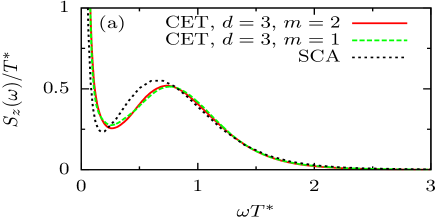
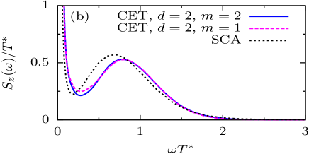
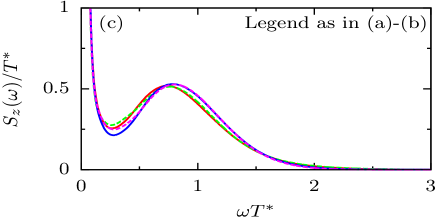
Figure 1: Analysis of the spin-noise spectrum $S_{z}(\omega)$ at zero external magnetic field. Comparison of $S_{z}(\omega)$ between the semiclassical approach (SCA) and fully quantum mechanical CET for two different envelope functions, $m=1,2$, and $d=3$ (a) and $d=2$ (b). Panel (c) combines the CET results of (a) and (b). For all CET calulations the ratio between the largest and smallest coupling constant has been set to $A_{\text{max}}/A_{\text{min}}=e^{9/4}$ and $S_{z}(\omega)$ has been averaged over $200$ individual QDs. For each QD, we included $N=18$ nuclear spins each coupled to the electron spin with a random coupling constant $A_{k}$ generated from $P(A)$ and the distribution of characteristic timescales. For the SCA we set $\tau_{s}=50T^{*}$.

Now we present a comparison of the spin-noise spectrum obtained from the fully quantum mechanical CET and SCA.

3.1 Zero external magnetic field

We begin with the results at $\bf B=0$. All approaches fulfil the spectral sum rule: the integrated spin-noise spectrum must be $1/4$, determined by the value of the autocorrelation function at $t=0$ [25]. We have used the time scale $T^{*}=\langle T^{*}(L_{0})\rangle$ as inverse unit of energy (frequency) in all of our plots where we present the spin noise spectra averaged over the distribution of QD radii. This averaging is denoted as $\langle\cdots\rangle$ in what follows.

Since the characteristic time scale $T^{*}\propto L_{0}^{d/2}$ depends on the QD dimension $d$, we present our results for a Gaussian ($m=2$) and exponential envelope function ($m=1$) for $d=3$ in Fig. 1(a) and for $d=2$ in Fig. 1(b). In order to compare the finite size CET calculations for the different electronic envelope functions, we determined the cutoff radius such that the ratio between the largest and the smallest hyperfine coupling in the simulation always remains at $A_{\text{max}}/A_{\text{min}}=e^{9/4}\approx 9.4877$.

In the SCA each individual QD is characterised by a Gaussian distribution of Overhauser fields whose width is determined by $T^{*}(L_{0})$. Consequently, the SCA results are only dependent of the dimension $d$ and the distribution of QD radii. We have obtained the distribution ${\cal F}(\vec{\Omega}_{N})$ entering Eq. (7) by averaging the radius dependent Gaussian over the distribution function of the radii, i. e. ${\cal F}(\vec{\Omega}_{N})=\langle{\cal F}[\vec{\Omega}_{N},T^{*}(L_{0})]\rangle$.

Figure 1(a) and (b) clearly show that the high-energy tails of the CET spin-noise spectrum $\mathcal{S}(\omega)$ are independent of the detailed shape of the envelope function and perfectly agrees with the SCA results. Only for low frequencies $\omega\ll 1/T^{*}$ deviations of the two approaches are observed. Those difference are related to the different treatment of the Overhauser field: While the SCA neglects the fluctuation of Overhauser field and performs the limit $N\to\infty$, the quantum mechanical CET includes the full dynamics of the small finite size nuclear spin. The slow precession of the individual nuclear spins yields a shift of the conserved spectral weight below the maximum $\omega T^{*}\approx 1/\sqrt{2}$ to lower frequencies in the CET. Furthermore, the slight differences in the noise spectra of $m=1$ and $m=2$ are related to the differences in the distribution function $P(A)$ given by Eq. (10).

In figure 1(c) we have combined the CET results of Fig. 1(a) and (b) for both dimensions. The overall qualitative agreement is remarkable. The high frequency tails, however, are clearly dependent on the dimension which can be traced back to the different scaling of $T^{*}(L_{0})\propto L_{0}^{d/2}$. We omitted the SCA results in Fig. 1(c) since the differences between the SCA data in 2D and 3D are similar to those of the CET and are also related to the scaling of $T^{*}(L_{0})$. The coincidence of $S(\omega)$ for $\omega\to 0$ is caused by the finite number of Chebyshev polynomials entering the CET approach. Detailed description of low frequency spin noise spectra is beyond the scope of the present paper [25].

3.2 Finite external magnetic field

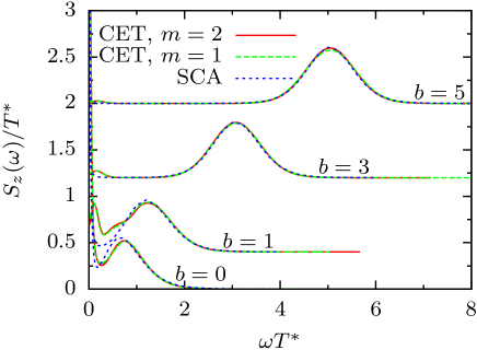
Figure 2: The spin correlation function $S_{z}(\omega)$ is shown for a varying external magnetic field applied along the $x$-direction, whose strength is given by $b=\omega_{L}T^{*}$. For clarity an offset proportional to $b$ has been added to the individual curves. All shown results are based on $d=3$ dimensional QDs and the ensemble average has been applied as described in the subset of Fig. 1. For the SCA we set $\tau_{s}=50T^{*}$.

Let us turn to the evolution of the spin-noise spectrum in a finite magnetic field applied in $x$-direction. In the presence of the magnetic field, the fluctuation spectra of transverse, $\mathcal{S}_{z}(\omega)$, $\mathcal{S}_{y}(\omega),$ and longitudinal, $\mathcal{S}_{x}(\omega),$ components become different [13]. In what follows we focus on the case of Voigh geometry and address the spin $z$-component noise spectrum, $\mathcal{S}_{z}(\omega)$. Since according to Fig. 1(c) there are only very subtle differences between the different dimensions, we restrict ourselves to $d=3$. We present a comparison of the SCA and the CET for three different dimensionless magnetic fields $b=\omega_{L}T^{*}=1,3,5$ in Fig. 2. For completeness, we have added the data of Fig. 1(a), i. e., the curves for $b=0$.

For $b=1$, the CET peak has almost approached the SCA curve. The only deviations at small frequencies are related to the spectra weight located in the $\omega=0$ peak. Namely, the CET faster shifts the weight of the non-decaying fraction of the autocorrelation function, originally described by the $\Delta(\omega)$-peak at $b=0$, to higher frequencies than the SCA. Futhermore, the application of the external magnetic field suppresses the quantum-fluctuation of the nuclear spin bath the stronger, the higher field strength $b$. At $b=3$, hardly any difference are observable and for $b=5$ we found perfect agreement between the CET and the SCA. The peak position in the spin-noise spectra is given by $\omega^{*}=\sqrt{\omega_{L}^{2}+(T^{*})^{-2}/2}$ and approaches the electron Larmor frequency $\omega_{L}$ only at large magnetic field, $\omega_{L}\gg 1/T^{*}$ [25].

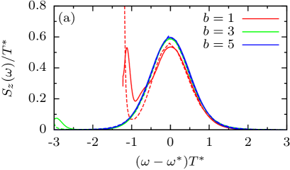
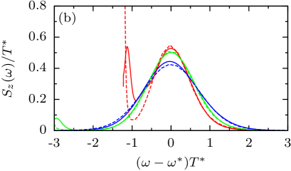
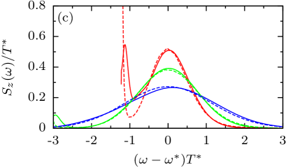
Figure 3: The spin correlation function $S_{z}(\omega)$ for three different a finite magnetic fields $b=1,3,5$ applied along the $x$-axis and different distributions of $g$ factors plotted as function of the shifted frequency $(\omega-\omega^{*})T^{*}$: (a) the same data as Fig. 2 for a fixed $g=g_{0}$, Gaussian distributions of $g$-factors with (b) $\Delta g/g_{0}=0.1$ and (c) $\Delta g/g_{0}=0.2$. The CET data are depicted as solid line, the SCA curves as dashed line of the same color. For the SCA we set $\tau_{s}=50T^{*}$.

So far, we have not taken into account the variation of the electronic $g$-factors in a QD ensemble. Owing to the size quantization effects, the the $g$-factor tensors of electron and holes in QDs show not only considerable derivations from isotropy but additionally vary with the size and shape of the QD [32]. Our aim here is to demonstrate qualitatively the effect of $g$-factor spread, hence, we are not trying to present a realistic modelling for a specific experiment. Hereafter consider the Voight geometry for the applied magnetic field only with magnetic field directed along one of the main axis of $g$-factor tensor, and a Gaussian distribution function

$$P(g)=\frac{1}{\Delta g\sqrt{2\pi}}\exp\left[-\frac{(g-g_{0})^{2}}{2(\Delta g)^{2}}\right],$$

onto the spin-noise spectrum, where $g_{0}$ is the average $g_{xx}$ component of $g$-factor tensor, $\Delta g$ is the width of the distribution.

Since the differences in $S_{z}(\omega)$ are subtle and vanish for large magnetic fields, we restrict our discussion on the impact of a $g$-factor distribution to the case $d=3$ and $m=2$. The results for two different values values $\Delta g/g=0.1,0.2$ and three different magnetic fields $b=1,3,5$ are depicted in Fig. 3. For completeness we added the data of Fig. 2(c) as panel (a), corresponding to $\Delta g=0$. The CET results are plotted as solid line, while the SCA data have been added as dashed line in the same color for the same magnetic field. By plotting in Fig. 3 the data as function of $(\omega-\omega^{*})T^{*}$, we clearly show that the finite frequency maxima are located at the analytically predicted effective Larmor frequency $\omega^{*}$ which approaches the bare Larmor frequency $\omega_{L}$ only at very large $b$-fields. For small fields, the spectral contribution near $\omega\approx 0$ remains visible. Upon increasing the spread of the $g$-factors, the broadening of the spin-noise peak at $\omega^{*}$ is increasing with increasing magnetic field as can be seen in Fig. 3(b) and 3(c). Again, the CET and the SCA agree perfectly at large magnetic fields.

4 Conclusion

We have presented a comparison of a semiclassical approach and fully quantum mechanical calculation of the spin-noise spectra of quantum dot ensembles. While the CET approach is limited to small bath sizes but treats the quantum fluctuations exactly, the SCA includes the correct limit $N\to\infty$ but neglects the nuclear spin dynamics.

We find a perfect agreement between both approaches for the high-frequency parts of the spin-noise spectra: the SCA and the CET predict the same short-time dynamics of the spin autocorrelation function. Since the CET includes the full quantum fluctuations of the nuclear spin bath the low frequency spectrum differs between the methods and is sensitive to the distribution function of the hyperfine coupling constants. Application of an external magnetic field suppresses quantum fluctuations and spin-noise spectra agree remarkably over the whole spectral range between both methods.

We acknowledge fruitful discussions with M. Bayer, A. Greilich, E.L. Ivchenko, D. Stanek, G. Uhrig, and D. Yakovlev. Partial support from RFBR, Russian Ministry of Education and Science (Contract No. 11.G34.31.0067 with SPbSU and leading scientist A. V. Kavokin) and Dynasty Foundation is acknowledged.

References

- [1] S. A. Crooker, J. Brandt, C. Sandfort, A. Greilich, D. R. Yakovlev, D. Reuter, A. D. Wieck, and M. Bayer, Phys. Rev. Lett. 104, 036601 (2010).
- [2] R. Dahbashi, J. Hübner, F. Berski, J. Wiegand, X. Marie, K. Pierz, H. W. Schumacher, and M. Oestreich, Appl. Phys. Lett. 100, 031906 (2012).
- [3] Y. Li, N. Sinitsyn, D. L. Smith, D. Reuter, A. D. Wieck, D. R. Yakovlev, M. Bayer, and S. A. Crooker, Phys. Rev. Lett. 108(May), 186603 (2012).
- [4] V. S. Zapasskii, A. Greilich, S. A. Crooker, Y. Li, G. G. Kozlov, D. R. Yakovlev, D. Reuter, A. D. Wieck, and M. Bayer, Phys. Rev. Lett. 110(Apr), 176601 (2013).
- [5] E. Aleksandrov and V. Zapasskii, Sov. Phys. JETP 54, 64 (1981).
- [6] M. Oestreich, M. Römer, R. J. Haug, and D. Hägele, Phys. Rev. Lett. 95(Nov), 216603 (2005).
- [7] G. M. Müller, M. Römer, D. Schuh, W. Wegscheider, J. Hübner, and M. Oestreich, Phys. Rev. Lett. 101(Nov), 206601 (2008).
- [8] V. S. Zapasskii, Adv. Opt. Photon. 5(2), 131–168 (2013).
- [9] J. Hübner, F. Berski, R. Dahbashi, and M. Oestreich, physica status solidi (b) pp. n/a–n/a (2014).
- [10] R. Hanson, L. P. Kouwenhoven, J. R. Petta, S. Tarucha, and L. M. K. Vandersypen, Rev. Mod. Phys. 79(4), 1217–1265 (2007).
- [11] J. Fischer, W. A. Coish, D. V. Bulaev, and D. Loss, Phys. Rev. B 78, 155329 (2008).
- [12] M. Gaudin, J. Physique 37, 1087 (1976).
- [13] M. M. Glazov and E. L. Ivchenko, Phys. Rev. B 86(Sep), 115308 (2012).
- [14] M. Bortz and J. Stolze, Phys. Rev. B 76(Jul), 014304 (2007).
- [15] A. Faribault and D. Schuricht, Phys. Rev. Lett. 110(Jan), 040405 (2013).
- [16] I. A. Merkulov, A. L. Efros, and M. Rosen, Phys. Rev. B 65(Apr), 205309 (2002).
- [17] A. Khaetskii, D. Loss, and L. Glazman, Phys. Rev. B 67(May), 195329 (2003).
- [18] K. A. Al-Hassanieh, V. V. Dobrovitski, E. Dagotto, and B. N. Harmon, Phys. Rev. Lett. 97(Jul), 037204 (2006).
- [19] G. Chen, D. L. Bergman, and L. Balents, Phys. Rev. B 76(Jul), 045312 (2007).
- [20] N. A. Sinitsyn, Y. Li, S. A. Crooker, A. Saxena, and D. L. Smith, Phys. Rev. Lett. 109(Oct), 166605 (2012).
- [21] D. Smirnov, M. Glazov, and E. Ivchenko, Physics of the Solid State 56(2), 254–262 (2014).
- [22] H. Tal-Ezer and R. Kosloff, J. Chem. Phys 81, 3967 (1984).
- [23] V. V. Dobrovitski and H. A. De Raedt, Phys. Rev. E 67(May), 056702 (2003).
- [24] A. Weiße, G. Wellein, A. Alvermann, and H. Fehske, Rev. Mod. Phys. 78(1), 275–306 (2006).
- [25] J. Hackmann and F. B. Anders, Phys. Rev. B 89(Jan), 045317 (2014).
- [26] D. Leonard, K. Pond, and P. M. Petroff, Phys. Rev. B 50(Oct), 11687–11692 (1994).
- [27] C. Testelin, F. Bernardot, B. Eble, and M. Chamarro, Phys. Rev. B 79(May), 195440 (2009).
- [28] U. Schollwöck, Annals of Physics 326(1), 96 – 192 (2011).
- [29] D. Stanek, C. Raas, and G. S. Uhrig, Phys. Rev. B 88(Oct), 155305 (2013).
- [30] M. M. Glazov, Journal of Applied Physics 113(13), – (2013).
- [31] W. A. Coish and D. Loss, Phys. Rev. B 70, 195340 (2004).
- [32] A. Schwan, B. M. Meiners, A. Greilich, D. R. Yakovlev, M. Bayer, A. D. B. Maia, A. A. Quivy, and A. B. Henriques, Applied Physics Letters 99(22), – (2011).