Bending dynamics of semi-flexible macromolecules in isotropic turbulence

Abstract

We study the Lagrangian dynamics of semi-flexible macromolecules in laminar as well as in homogeneous and isotropic turbulent flows by means of analytically solvable stochastic models and direct numerical simulations. The statistics of the bending angle is qualitatively different in laminar and turbulent flows and exhibits a strong dependence on the topology of the velocity field. In particular, in two-dimensional turbulence, particles are either found in a fully extended or in a fully folded configuration; in three dimensions, the predominant configuration is the fully extended one.

The study of hydrodynamic turbulence and of turbulent transport has received considerable impulse from the development of experimental, theoretical, and numerical Lagrangian techniques FGV01 ; TB09 ; PPR09 ; SC09 . The translational dynamics of tracer and inertial particles is indeed related to the mixing properties of turbulent flows BBBCMT06 and has applications in geophysics (atmospheric pollution, rain formation) S03 , astrophysics (dynamo effect, planet formation) CG95 ; A10 , and chemical engineering FT11 . Over the last decade, attention has extended to the Lagrangian dynamics of particles possessing additional degrees of freedom, such as elastic polymers and nonspherical solid particles (see, e.g., Refs. MV11 ; V13 and references therein). In particular, the examination of the extensional dynamics of polymers has provided information on the coil-stretch transition and on turbulent drag reduction S09 ; recent studies of the dynamics of non-spherical particles in isotropic turbulence have investigated the alignment and rotation statistics of such particles PW11 ; PCTV12 ; GVP13 ; CM13 ; GEM14 . In this Letter, we consider particles that possess yet another degree of freedom, namely semi-flexible macromolecules that can bend under the action of a non-uniform velocity field. We model a semi-flexible macromolecule as a trumbbell, i.e., as three beads connected by two rigid links H74 ; the stiffness of the trumbbell is controlled by an elastic hinge, which prevents the particle from bending. The trumbbell model (also known as trimer or three-bead-two-rod model) qualitatively captures the viscoelastic properties of suspensions of segmentally flexible macromolecules H74 ; BHAC77 ; RZ84 ; R84 ; NY85 ; R87 ; GT94 . This model also plays an important role in statistical mechanics as the prototypical system for showing that the infinite-stiffness limit of elastic bonds is singular H74 ; GB76 ; H79 ; R79 ; H94 . Moreover, an active variant of the trumbbell model, the trumbbell swimmer, describes the swimming motion of certain biological microorganisms NG04+GA08 ; NRY13 (see also Ref. SN11 ). We study the bending dynamics of trumbbells, in both laminar and fully turbulent flows, via analytical calculations and detailed numerical simulations, and show that the statistics of the bending angle depends strongly on the topology of the flow. In particular, in a two-dimensional (2D) homogeneous and isotropic, incompressible turbulent flow, the configurations in which the rods are parallel or antiparallel are the most probable ones; as the amplitude of the velocity gradient increases, these probabilities become sharper, with the parallel configuration becoming the most likely for very strong turbulence. By contrast, in three dimensions, the antiparallel configuration always is the most probable one.

A trumbbell consists of three spherical beads joined by two inertialess rigid rods of equal length $\ell$ immersed in a Newtonian fluid (Fig. 1) H74 ; BHAC77 .

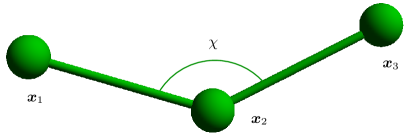
Figure 1: (color online) The trumbbell model.

The drag force acting on each of the beads is given by the Stokes law with a drag coefficient $\zeta$. An elastic hinge at the middle of the trumbbell models the action of the entropic forces which prevent the trumbbell from bending; the force exerted by the elastic hinge is described by a harmonic potential. The maximum end-to-end extension of the trumbbell, $2\ell$, is sufficiently small for (a) it to experience Brownian fluctuations and (b) the velocity gradient $\nabla\bm{u}$ to be spatially uniform across the trumbbell. The inertia of the beads and the hydrodynamic interactions between them are disregarded. Furthermore, the suspension is assumed to be sufficiently dilute; hence, particle-particle hydrodynamic interactions are negligible.

The positions of the beads are denoted as $\bm{x}_{i}$, $i=1,2,3$. Under the above assumptions, the position of the center of mass, $\bm{x}_{c}\equiv(\bm{x}_{1}+\bm{x}_{2}+\bm{x}_{3})/3$, evolves like that of a tracer, i.e., $\dot{\bm{x}}_{c}(t)=\bm{u}(\bm{x}_{c}(t),t)$. The separation vectors between the beads and the center of mass are defined as $\bm{r}_{\nu}\equiv\bm{x}_{\nu}-\bm{x}_{c}$ with $\nu=1,2,3$. However, the configuration of the trumbbell in the reference frame of the center of mass is more conveniently described in terms of a reduced set of $2(d-1)$ angular coordinates $\bm{q}$, where $d$ is the dimension of the fluid BHAC77 . For $d=2$, $\bm{q}=(\theta,\chi)$ where $0\leqslant\theta<2\pi$ gives the orientation of the vector $\bm{x}_{3}-\bm{x}_{2}$ with respect to a fixed frame of reference and $0\leqslant\chi<\pi$ is the internal angle between $\bm{x}_{1}-\bm{x}_{2}$ and $\bm{x}_{3}-\bm{x}_{2}$ (Fig. 1). By letting $\chi$ vary between 0 and $\pi$ only, we do not distinguish between the two configurations that are obtained by exchanging $\bm{x}_{1}$ and $\bm{x}_{3}$. The separation vectors $\bm{r}_{\nu}$ are expressed in terms of $\theta$ and $\chi$ as follows:

$$\begin{array}[]{l}\bm{r}_{1}=\frac{\ell}{3}\left(2\cos(\theta+\chi)-\cos(\theta),2\sin(\theta+\chi)-\sin(\theta)\right),\\ \bm{r}_{2}=-\frac{\ell}{3}\left(\cos(\theta+\chi)+\cos(\theta),\sin(\theta+\chi)+\sin(\theta)\right),\\ \bm{r}_{3}=\frac{\ell}{3}\left(2\cos(\theta)-\cos(\theta+\chi),2\sin(\theta)-\sin(\theta+\chi)\right).\end{array}$$ (1)

For $d=3$, $\bm{q}=(\alpha,\beta,\gamma,\chi)$ where $0\leqslant\chi<\pi$ is once again the internal angle between the two rods (Fig. 1) and $0\leqslant\alpha,\gamma<2\pi$, $0\leqslant\beta<\pi$ are the Euler angles that specify the absolute orientation of the orthogonal triad $(\bm{x}_{3}-\bm{x}_{1})\wedge(\bm{x}_{2}-\bm{x}_{c})$, $\bm{x}_{3}-\bm{x}_{1}$, $\bm{x}_{2}-\bm{x}_{c}$ with respect to a fixed coordinate system (for the relation between $\bm{r}_{\nu}$ and $\bm{q}$ in three dimensions, see Refs. H74 ; BHAC77 ).

The statistics of the configuration of the trumbell is specified by the distribution function $\psi(\bm{q};t)$, which is such that $\psi(\bm{q};t)Jd\bm{q}$ is the probability that, at time $t$, the angular variables describing the configuration lie in the range $\bm{q}$ to $\bm{q}+d\bm{q}$. Here, $J$ is the Jacobian of the transformation from the coordinates $\bm{r}_{\nu}$ to the coordinates $\bm{q}$: $J=1$ for $d=2$ and $J=\sin\chi\sin\beta$ for $d=3$. Furthermore, $\psi(\bm{q};t)$ is normalized as $\int\psi(\bm{q};t)Jd\bm{q}=1$. For a deterministic flow, $\psi(\bm{q};t)$ satisfies the following convection-diffusion equation BHAC77 (summation over repeated indices is understood throughout this Letter):

$$\dfrac{\partial\psi}{\partial t}=-\dfrac{1}{J}\dfrac{\partial}{\partial q^{i}}\left\{J\mathcal{G}^{ij}\left[\left(\kappa^{kl}(t)r_{\nu}^{l}\dfrac{\partial r_{\nu}^{k}}{\partial q^{j}}-\dfrac{1}{\zeta}\dfrac{\partial\phi}{\partial q^{j}}\right)\psi\right.\right.\\ -\left.\left.\dfrac{KT}{\zeta}\sqrt{h}\dfrac{\partial}{\partial q^{j}}\left(\dfrac{J\psi}{\sqrt{h}}\right)\right]\right\},$$ (2)

where $\kappa^{ij}(t)=\partial^{j}u^{i}(t)$ is the velocity gradient evaluated at $\bm{x}_{c}(t)$, $K$ is the Boltzmann constant, $T$ is temperature, $\phi=\mu(\chi-\pi)^{2}/2$ is the bending potential, $\mathcal{G}=\mathcal{H}^{-1}$ with $\mathcal{H}^{ij}=\frac{\partial r^{k}_{\nu}}{\partial q^{i}}\frac{\partial r^{k}_{\nu}}{\partial q^{j}},$ and $h=\operatorname{det}(\mathcal{H})$. As $\bm{q}$ are angular variables, $\psi(\bm{q};t)$ satisfies periodic boundary conditions.

In the absence of flow ($\bm{\kappa}=0$) and of bending potential ($\mu=0$), the stationary form of $\psi(\bm{q};t)$ is $\psi_{\mathrm{st}}(\chi)=N\psi_{0}(\chi)$ with $\psi_{0}(\chi)=\sqrt{4-\cos^{2}\chi}$ H74 (throughout this Letter, $N$ denotes a normalization constant). Thus, the most probable configuration is that with the rods being perpendicular ($\chi=\pi/2$); the parallel ($\chi=0$) and antiparallel ($\chi=\pi$) configurations are equally probable, but their probability is about 15% smaller. The bending potential breaks the aforementioned symmetry. For $\mu\neq 0$, $\psi_{\mathrm{st}}(\chi)=N\psi_{0}(\chi)\exp\left[-Z(\pi-\chi)^{2}/2\right]$ H74 , where $Z\equiv\mu/KT$ is a stiffness parameter and determines the equilibrium configuration of the trumbbell. Thus, the probability of the $\chi=\pi$ configuration increases as $Z$ increases. Finally, when the trumbbell is immersed in a non-uniform flow ($\bm{\kappa}(t)\neq 0$) its dynamics results from the interplay between the restoring action of the elastic hinge and the deformation by the flow.

We first examine the effect of pure stretching on the statistics of the bending angle. Consider a 2D hyperbolic velocity field $\bm{u}(x,y)=\sigma(x,-y)$. This flow is potential, i.e., $\bm{\kappa}=\bm{\kappa}^{\mathrm{T}}$. Therefore, the stationary solution of Eq. (2) takes the form: $\psi_{\mathrm{st}}(\theta,\chi)=N\sqrt{h}\exp[(\Phi-\phi)/KT]$, where $\Phi=(\zeta/2)\sum_{\nu}\kappa^{ij}r^{i}_{\nu}r^{j}_{\nu}$ K44 ; H74 . The function $\psi_{\mathrm{st}}$ is shown in Fig. 2(a) for representative values of the parameters.

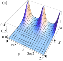
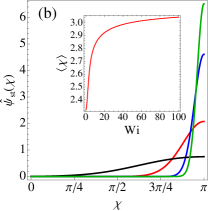
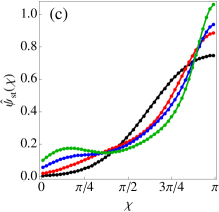
Figure 2: (color online) 2D hyperbolic flow : (a) surface plot of $\psi_{\mathrm{st}}(\theta,\chi)$ for $Z=1$ and $\mathrm{Wi}=2$. For $Z=1$ and $\mathrm{Wi}=0$, $\langle\chi\rangle\approx 2.32$, slightly less than $3\pi/4$; (b) Marginal distribution of $\chi$ for $Z=1$ and $\mathrm{Wi}=0$ (black), $\mathrm{Wi}=10$ (red), $\mathrm{Wi}=50$ (blue), $\mathrm{Wi}=100$ (green). The inset shows the average of $\chi$ vs. $\mathrm{Wi}$ for $Z=1$. (c) Marginal distribution of $\chi$ for $Z=1$ and $\mathrm{Wi}=0$ (black), $\mathrm{Wi}=10$ (red), $\mathrm{Wi}=50$ (blue), $\mathrm{Wi}=100$ (green) for a 2D simple shear flow.

Since $\psi_{\mathrm{st}}$ depends on both $\chi$ and $\theta$, the statistics of the bending angle varies according to the orientation of the trumbbell with respect to the stretching direction of the flow. However, the average effect of the hyperbolic flow can be understood by considering the marginal distribution $\widehat{\psi}_{\mathrm{st}}(\chi)\equiv\int_{0}^{2\pi}\psi_{\mathrm{st}}(\theta,\chi)d\theta$, which can be written explictly as follows:

$$\textstyle\widehat{\psi}_{\mathrm{st}}(\chi)=N\psi_{0}(\chi)\exp\left[-\frac{Z}{2}(\pi-\chi)^{2}\right]I_{0}\left(\textstyle\frac{Z(1-2\cos\chi)\mathrm{Wi}}{3}\right),$$ (3)

where $I_{0}$ is the modified Bessel function of the first kind of order 0 and $\mathrm{Wi}=\sigma\tau$ (here $\tau=\zeta\ell^{2}/\mu$ is the characteristic time scale of the bending potential) foot1 . The Weissenberg number $\mathrm{Wi}$ measures the relative strength of the flow and of the bending potential. Since the function $I_{0}(z)$ is even, decreases with $z$ for $z<0$ and increases for $z>0$, on average the hyperbolic flow favors the $\chi=\pi$ configuration. Hence it strengthens the action of the entropic forces and this effect becomes stronger as $\mathrm{Wi}$ increases (Fig. 2(b)). An analogous analysis for a three-dimensional (3D) incompressible hyperbolic flow shows that the stationary statistics of $\chi$ exhibits similar properties in two and in three dimensions.

In a hyperbolic flow, a trumbbell is subject only to pure stretching. However, most practical flows have a rotational component as well. A purely rotational planar flow, $\bm{u}(x,y)=\sigma(y,-x)$, has no effect on the stationary statistics of $\chi$. Indeed, for this flow, the convective term in Eq. (2) has zero $\chi$-component, and hence $\psi(\theta,\chi;t)$ converges in time to the stationary solution of the $\mathrm{Wi}=0$ case. However, the combined effect of stretching and rotation can influence the bending dynamics. To illustrate this fact, we consider a simple shear $\bm{u}(x,y)=\sigma(y,0)$, which is the superposition of a purely extensional component and of a purely rotational component with equal magnitudes. If the flow is not potential, no general analytical expression is available for $\psi_{\mathrm{st}}(\theta,\chi)$. Thus we compute $\widehat{\psi}_{\mathrm{st}}(\chi)$ from a Monte Carlo numerical simulation of Eq. (2). Figure 2(c) shows that the $\chi=\pi$ configuration is the most probable one for all the values of $\mathrm{Wi}$ considered. As $\mathrm{Wi}$ increases, the interplay between rotation and stretching increases the probability of the small-$\chi$ configurations, unlike the purely extensional flow where it is negligible. However, for a given $\mathrm{Wi}$, the ability of the shear flow to bend a trumbbell is less than that of an hyperbolic flow with comparable $\mathrm{Wi}$.

In a random or turbulent flow, the extensional and rotational components of the velocity gradient fluctuate in time and in space. The above analysis suggests that the combination of these two components may generate a complex bending dynamics. In order to examine this point analytically, we consider the Kraichnan random flow K68 in the Batchelor regime (see also Ref. FGV01 ). The velocity gradient $\bm{\kappa}(t)$ is a delta-correlated-in-time $(d\times d)$-dimensional Gaussian stochastic process with zero mean and correlation: $\langle\kappa^{ij}(t)\kappa^{kl}(t^{\prime})\rangle=\mathcal{K}^{ijkl}\delta(t-t^{\prime})$, where $\mathcal{K}^{ijkl}=2\lambda[(d+1)\delta^{ik}\delta^{jl}-\delta^{ij}\delta^{kl}-\delta^{il}\delta^{jk}]/[d(d-1)]$ and $\lambda$ is the maximum Lyapunov exponent of the flow. The form of the tensor $\mathcal{K}$ ensures that the flow is incompressible and statistically isotropic. Although the assumption of temporal decorrelation is unrealistic, the study of this flow has contributed in a substantial way to the understanding of turbulent transport (e.g., of passive scalars, magnetic fields, and elastic polymers), because it allows an analytical approach to this problem FGV01 . We denote by $P(\bm{q};t)$ the distribution of the configuration of the trumbbell with respect to the realizations of both $\bm{\kappa}(t)$ and thermal noise; $P(\bm{q};t)$ is normalized as $\int P(\bm{q};t)Jd\bm{q}=1$. A Gaussian integration by part of Eq. (2) (e.g., Ref. F95 ) yields the following equation for $P(\bm{q};t)$:

$$\dfrac{\partial P}{\partial t}=\dfrac{\partial}{\partial q^{i}}\left\{\dfrac{1}{2}\mathcal{K}^{klmn}\mathcal{G}^{ij}r_{\nu}^{l}\dfrac{\partial r_{\nu}^{k}}{\partial q^{j}}\dfrac{\partial}{\partial q^{a}}\left(\mathcal{G}^{ab}r_{\rho}^{n}\dfrac{\partial r_{\rho}^{m}}{\partial q^{b}}P\right)+\right.\\ \left.\frac{\mathcal{G}^{ij}}{\zeta}\left[\dfrac{\partial\phi}{\partial q^{j}}P+KT\sqrt{h}\dfrac{\partial}{\partial q^{j}}\left(\dfrac{P}{\sqrt{h}}\right)\right]\right\},$$ (4)

which must be solved with periodic boundary conditions.

Let us first consider the 2D case. When $\bm{q}=(\theta,\chi)$, $J=1$, and the corresponding $\mathcal{G}$ are substituted into Eq. (4), we can rewrite Eq. (4) as a Fokker-Planck equation (FPE) in the two variables $\theta$ and $\chi$. The drift and diffusion coefficients, however, do not depend on $\theta$ as a consequence of the statistical isotropy of the flow. Hence the stationary distribution of the configuration is a function of $\chi$ alone and is the stationary solution of the following FPE in one variable:

$$\partial_{s}P=-\partial_{\chi}(V_{\chi}P)+\textstyle\frac{1}{2}\partial^{2}_{\chi\chi}(D_{\chi\chi}P),$$ (5)

where $s=t/\tau$,

$$V_{\chi}(\chi)=\frac{12\sin\chi}{Z\left(2-\cos\chi\right)\left(2+\cos\chi\right)^{2}}+\frac{6\left(\pi-\chi\right)}{\left(2+\cos\chi\right)}+\\ 2\mathrm{Wi}\,\frac{\sin\chi[5+\cos\chi-11\cos(2\chi)-\cos(3\chi)]}{\left(2-\cos\chi\right)\left(2+\cos\chi\right)^{3}},$$ (6)

and

$$D_{\chi\chi}(\chi)=\frac{12}{Z\left(2+\cos\chi\right)}+\mathrm{Wi}\,\frac{16\sin^{2}\chi}{\left(2+\cos\chi\right)^{2}}.$$ (7)

In a random flow, the time scale associated with stretching is given by $\lambda$; accordingly, in Eqs. (6) and (7) $\mathrm{Wi}=\lambda\tau$. The stationary solution of Eq. (5) that satisfies periodic boundary conditions is R89 :

$$P_{\mathrm{st}}(\chi)=\dfrac{N}{D_{\chi\chi}(\chi)}\exp\left(2\int_{0}^{\chi}\dfrac{V_{\chi}(\eta)}{D_{\chi\chi}(\eta)}\,d\eta\right).$$ (8)

The function $P_{\mathrm{st}}(\chi)$ is plotted in Fig. 3(a) for different values of $\mathrm{Wi}$. For small $\mathrm{Wi}$, the most probable configuration is the antiparallel one, as in the hyperbolic flow. However, as $\mathrm{Wi}$ increases, a second peak emerges near $\chi=0$, while intermediate values of $\chi$ become less and less probable. At large Wi, $P_{\mathrm{st}}(\chi)$ consists of two narrow peaks, one at $\chi=\pi$ and the other approaching $\chi=0$, with the latter becoming more and more pronounced as Wi increases (Fig. 3(a)).

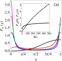
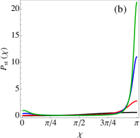
Figure 3: (color online) Stationary distribution function of $\chi$ for the Batchelor-Kraichnan flow with $Z=1$ and $\mathrm{Wi}=0$ (black), $\mathrm{Wi}=10$ (red), $\mathrm{Wi}=50$ (blue), $\mathrm{Wi}=100$ (green), and $\mathrm{Wi}=150$ (magenta) in (a) two and (b) three dimensions. The inset in (a) shows the values of $P_{\mathrm{st}}(\chi)$ at $\chi=0$ (dashed line) and $\chi=\pi$ (solid line) as a function of $\mathrm{Wi}$.

It is important to ask if the results above carry over to the 3D Batchelor-Kraichnan flow. In three dimensions, Eq. (4) can be rewritten as a FPE in the four variables $\alpha,\beta,\gamma,\chi$. As a consequence of the statistical isotropy of the flow, the stationary distribution of the configuration, $P_{\mathrm{st}}(\bm{q})$, depends only on $\chi$. In particular, $P_{\mathrm{st}}(\chi)\sin\chi$ is again the stationary solution of a FPE in one variable. Figure 3(b) shows $P_{\mathrm{st}}(\chi)$ for different values of $\mathrm{Wi}$. A small peak at $\chi=0$ emerges only for very large values of $\mathrm{Wi}$; the $\chi=\pi$ configuration prevails for all values of $\mathrm{Wi}$ (Fig. 3(b)). Thus, the statistics of $\chi$ is different in two and three dimensions. In particular, for $d=3$, the behavior of the distribution of $\chi$ is qualitatively similar to that in the purely extensional flow.

Are the results obtained so far for model flows valid in realistic, turbulent flows? To ensure that the qualitative properties of the statistics of $\chi$ do not depend on the Gaussianity and temporal decorrelation of the Batchelor-Kraichnan flow, we perform a Lagrangian direct numerical simulation of the trumbbell model in a 2D, incompressible turbulent flow. Our direct numerical simulation of the forced (at large scale) incompressible, 2D Navier-Stokes equation uses a pseudospectral method pseudo and a second-order, exponential Runge-Kutta scheme  cox+mat02 , with $1024^{2}$ collocation points and the $2/3$ dealiasing rule on a 2$\pi$-periodic square domain. We present representative results from a simulation where the choice of the forcing amplitude, the coefficient of the Ekman friction, and the kinematic viscosity yield a Taylor-microscale Reynolds number $\mathrm{Re}_{\lambda}\approx 827$, in the non-equilibrium, statistically steady state; we have done several other simulations with different $\mathrm{Re}_{\lambda}$ and forcing scales which yield results consistent with the ones presented here. This flow is seeded with $10^{3}$ independently evolving trumbbells each of whose center of mass evolves as a Lagrangian tracer particle; the velocity at $\bm{x}_{c}$, is evaluated from the Eulerian velocity by using a bilinear-interpolation scheme pp11 . The Lagrangian evolution of the configuration of the trumbbell is once again computed from a Monte Carlo simulation of Eq. (2). We define the Weissenberg number as $\mathrm{Wi}=\tau/\tau_{\mathrm{min}}$, where $\tau_{\mathrm{min}}$ is the smallest time scale associated with the direct cascade of enstrophy and is estimated as the minimum value of $(\sqrt{k^{3}E(k)})^{-1}$ BS02 (here $E(k)$ denotes the isotropic kinetic-energy spectrum).

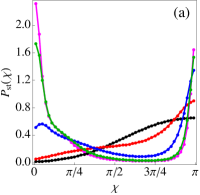
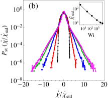
Figure 4: (color online) 2D homogeneous, isotropic, turbulence: (a) distribution of $\chi$ for $Z=1$ and $\mathrm{Wi}\approx 3$ (black), $\mathrm{Wi}\approx 167$ (red), $\mathrm{Wi}\approx 10^{3}$ (blue), $\mathrm{Wi}\approx 3.3\times 10^{3}$ (green), $\mathrm{Wi}\approx 6.6\times 10^{3}$ (magenta) and (b) distribution of $\dot{\chi}/\dot{\chi}_{\rm std}$ for $Z=1$ for different values of $\mathrm{Wi}$ [same as in panel (a)] and the dependence of $\dot{\chi}_{\rm std}$ on $\mathrm{Wi}$.

Figure 4(a) shows the distribution function of the internal angle $\chi$; the statistics of $\chi$ qualitatively agrees with that calculated for the 2D Batchelor-Kraichnan random flow. In particular, we find that at small $\mathrm{Wi}$, the antiparallel configuration is favoured; with increasing $\mathrm{Wi}$, the probability of being in a parallel configuration increases significantly and eventually, at extremely large values of $\mathrm{Wi}$, the distribution function displays strong peaks at both $\chi\approx 0$ and $\chi\approx\pi$. We also calculate the distribution function of the rate of change of the angle $\dot{\chi}$, normalised by its standard deviation $\dot{\chi}_{\rm std}$, for various values of $\mathrm{Wi}$. With increasing $\mathrm{Wi}$ (Fig. 4(b)), the distribution function, which is symmetric and peaked at $\dot{\chi}\approx 0$, develops exponential tails. The standard deviation itself, $\dot{\chi}_{\rm std}$, is a decreasing function of $\mathrm{Wi}$ (Fig. 4(b), inset).

In this Letter, by using analytical calculations and numerical simulations, we have shown how the conformation of semiflexible macromolecules, modelled via the trumbbells, can change with $\mathrm{Wi}$ as well as the flow topology. The statistics of the bending angle in turbulent or random flows depends strongly on the space dimension and is qualitatively different from that observed in simple laminar flows. This fact suggests that the rheology of semiflexible macromolecules also exhibits a strong dependence on the turbulent character of the flow and on its spatial dimension. The recent advances in Lagrangian experimental techniques allow extensive laboratory studies of the deformation of macromolecules in turbulent flows TB09 ; S09 . We hope our work would lead to further experiments directed towards the study of the Lagrangian dynamics of semi-flexible macromolecules in turbulent flows and the non-Newtonian properties of turbulent suspensions of such particles.

- (1) G. Falkovich, K. Gawȩdzki, and M. Vergassola, Rev. Mod. Phys. 73, 913 (2001).
- (2) R. Pandit, P. Perlekar, and S.S. Ray, Pramana 73, 157 (2009).
- (3) J.P.L.C. Salazar and L.R. Collins, Annu. Rev. Fluid Mech. 41, 405 (2009).
- (4) F. Toschi and E. Bodenschatz, Annu. Rev. Fluid Mech. 41, 375 (2009).
- (5) J. Bec, L. Biferale, G. Boffetta, M. Cencini, S. Musacchio and F. Toschi, Phys. Fluids 18, 091702 (2006).
- (6) R. Shaw, Annu. Rev. Fluid Mech. 35, 183 (2003).
- (7) S. Childress and A.D. Gilbert, Stretch, Twist, Fold: The Fast Dynamo (Springer-Verlag, Berlin, Heidelberg, 1995).
- (8) P.J. Armitage, Astrophysics of Planet Formation (Cambridge University Press, Cambridge, England, 2010).
- (9) M.D. Finn and J.-L. Thiffeault, SIAM Rev. 53, 723 (2011).
- (10) S. Musacchio and D. Vincenzi, J. Fluid Mech. 670, 326 (2011).
- (11) D. Vincenzi, J. Fluid Mech. 719, 465 (2013).
- (12) V. Steinberg, C. R. Physique 10, 728 (2009).
- (13) A. Pumir and M. Wilkinson, New J. Phys. 13, 093030 (2011).
- (14) S. Parsa, E. Calzavarini, F. Toschi, and G.A. Voth, Phys. Rev. Lett. 109, 134501 (2012).
- (15) L. Chevillard and C. Meneveau, J. Fluid Mech. 737, 571 (2013).
- (16) K. Gustavsson, J. Einarsson, and B. Mehlig, Phys. Rev. Lett. 112, 014501 (2014).
- (17) A. Gupta, D. Vincenzi and R. Pandit, Phys. Rev. E 89, 021001(R) (2014).
- (18) O. Hassager, J. Chem. Phys. 60, 2111 (1974); ibid. 60, 4001 (1974).
- (19) R.B. Bird, O. Hassager, R.C. Armstrong, and C.F.C. Curtiss, Dynamics of Polymeric Liquids (Wiley, New York, 1977), Vol. 2.
- (20) D.B. Roitman and B.H. Zimm, J. Chem. Phys. 81, 6333 (1984); ibid. 81, 6348 (1984).
- (21) D.B. Roitman, J. Chem. Phys. 81, 6356 (1984).
- (22) K. Nagasaka and H. Yamakawa, J. Chem. Phys. 83, 6480 (1985).
- (23) D.B. Roitman, Lect. Notes Phys. 283, 192 (1987).
- (24) J. Garcia de la Torre, Eur. Biophys. J. 23, 307 (1994).
- (25) M. Gottlieb and R.B. Bird, J. Chem. Phys. 65, 2467 (1976).
- (26) E. Helfand, J. Chem. Phys. 71, 5000 (1979).
- (27) J.M. Rallison, J. Fluid Mech. 93, 251 (1979).
- (28) E.J. Hinch, J. Fluid Mech. 271, 219 (1994)
- (29) A. Najafi and R. Golestanian, Phys. Rev. E 69, 062901 (2004); R. Golestanian and A. Ajdari, ibid. 77, 036308 (2008).
- (30) A. Najafi, S.S.H. Raad, R. Yousefi, Phys. Rev. E 88, 045001 (2013).
- (31) G. Subramanian and P.R. Nott, J. Indian Inst. Sci. 91, 383 (2011).
- (32) H.A. Kramers, Physica 11, 1 (1944).
- (33) For , Eq. (2) describes Hassager’s free-hinge model H74 ; the statistics of for the free-hinge model can be derived from our results by letting tend to zero while keeping constant.
- (34) R.H. Kraichnan, Phys. Fluids 11, 945 (1968).
- (35) U. Frisch, Turbulence: The Legacy of Kolmogorov (Cambridge University Press, Cambridge, England, 1995).
- (36) H. Risken, The Fokker-Planck equation (Springer-Verlag, 1989).
- (37) C. Canuto, M.Y. Hussaini, A. Quarteroni and T.A. Zang, Spectral methods in Fluid Dynamics (Spinger-Verlag, Berlin, 1988).
- (38) S. M. Cox and P. C. Matthews, J. Comput. Phys. 176, 430 (2002).
- (39) P. Perlekar, S. S. Ray, D. Mitra, and R. Pandit, Phy. Rev. Lett. 106, 054501 (2011); S. S. Ray, D. Mitra, P. Perlekar, and R. Pandit, Phys. Rev. Lett. 107, 184503 (2011).
- (40) G. Boffetta and I.M. Sokolov, Phys. Fluids 14, 3224 (2002).