An invitation to trees of finite cone type: random and deterministic operators

Abstract.

Trees of finite cone type have appeared in various contexts. In particular, they come up as simplified models of regular tessellations of the hyperbolic plane. The spectral theory of the associated Laplacians can thus be seen as induced by geometry. Here we give an introduction focusing on background and then turn to recent results for (random) perturbations of trees of finite cone type and their spectral theory.

1. Introduction

Trees of finite cone type are a generalization of regular trees. They have a special form of ’recursive structure’. Over the years they have appeared in various contexts. These include – in the order of appearance – the following:

• Theory of random walks.

• Spectral theory of hyperbolic tessellations.

• Random Schrödinger operators.

Here, we want to give an introduction into the topic. In particular, we want to illuminate each of these contexts and provide some background. Our main results then concern (random) Schrödinger operators associated to such trees.

More specifically, this article will deal with the following questions in the indicated sections.

• What are trees of finite cone type? (Section 2).

• Why study trees of finite cone type? (Section 3).

• Which spectral properties have trees of finite cone type? (Section 4).

• How are trees of finite cone type related to multi-type Galton Watson trees? (Section 5).

Finally, we will present some ideas behind the proofs in Section 6.

The results in Section 4 are published in [KLW, KLW2]. These works in turn rely on the PhD thesis of one of the authors (M.K.). The results of Section 5 for Galton Watson type trees can be found in [Kel2].

Acknowledgments. D.L. and S.W. take this opportunity to express their heartfelt thanks to the organizers of Pasturfest (2013) in Hagen. Furthermore, M.K. would like to thank Balint Virag for the very inspiring discussions during his visit in Toronto leading to simplifications of the proofs presented in this survey.

2. What are trees of finite cone type?

In this section we introduce trees of finite cone type. We will assume familiarity with basic notions from graph theory and just remind the reader of certain notions.

For us a graph is a pair $(V,E)$ consisting of a set $V$ called vertices and a set $E$ called edges consisting of subsets of $V$ with exactly two elements. For $x,y\in V$, we will write $x\sim y$ if $\{x,y\}\in E$ and call $x$ and $y$ neighbors. The number of neighbors of $x$ is called the degree of $x$.

A finite sequence $x_{0},x_{1},\ldots,x_{n}$ of pairwise different vertices is called a path of length $n$ connecting $x_{0}$ and $x_{n}$ if $x_{j}\sim x_{j+1}$ holds for all $j=0,\ldots,n-1$. If any two vertices are connected by a path, then the graph is called connected. In this case, the distance between two vertices is the length of the shortest path connecting these vertices. If for any two vertices there exists exactly one path connecting them (thus the graph is connected without loops), then the graph is called a tree and the unique path between two vertices is called a geodesic. A connected graph with a distinguished vertex is called a rooted graph and the distinguished vertex is called the root.

In a rooted tree (i.e., a tree with a root) the elements with distance $n$ to the root are called $n$-sphere. A neighbor of a vertex $v$ in the $n$-sphere is called a forward neighbor if it belongs to the $(n+1)$-sphere. The cone, or rather forward cone, of a vertex $v$ in a rooted tree is then the smallest subgraph of the rooted tree which contains $v$ and all forward neighbors of any of its vertices. A rooted tree is called regular if the number of forward neighbors of any vertex is constant.

We will deal with graphs in which every vertex is labeled. This means we will have a map from the vertices to some (finite) set called the labels.

Trees of finite cone type arise from the following two pieces of data:

• A finite set $\mathcal{A}$ called vertex labels.

• A map $M:\mathcal{A}\times\mathcal{A}\longrightarrow{\mathbb{N}}_{0}$ called substitution rule.

Given these data we can then construct a rooted tree ${\mathbb{T}}={\mathbb{T}}(M,j)$ whose vertices carry labels from $\mathcal{A}$ and whose root is labeled by $j$ in the following way:

Every vertex with label $k$ of the $n$-sphere is joined to $M_{l,k}$ vertices of label $l$ of the $(n+1)$-sphere.

The arising structure is obviously a rooted tree in which every vertex has a label. By construction the cone of any vertex is completely determined by the label of the vertex. In particular, there are only finitely many different types of cones present. Conversely, it is not hard to see that any rooted tree with the property that it has only finitely many types of cones arises in the manner described above. We will refer to such trees as trees of finite cone type. By construction the vertex degree is uniformly bounded in a tree of finite cone type.

Note that our data allows us to constructed one tree for each element of $\mathcal{A}$.

Remark. As already mentioned in the introduction, trees of finite cone type have come up in several contexts. In fact, they have also been denoted as periodic trees or as monoids with certain properties. Here, we follow Nagnibeda / Woess [NW] in calling them trees of finite cone type.

In order to achieve a meaningful theory we will impose the following assumptions on our data or more precisely on the substitution matrix $M$:

• If $\mathcal{A}$ consists of only one point, then $M=M_{1,1}\geq 2$ (not one-dimensional),

• $M_{j,j}\geq 1$ for all $j\in{\mathcal{A}}$ (positive diagonal),

• there exists $n=n(M)$ with $M^{n}$ has positive entries (primitivity).

Remark. Due to positivity of diagonal primitivity follows already from a generally weaker condition known as irreducibility.

Let us discuss a concrete example, which we call the Fibonacci tree.

Example 2.1.

Let ${\mathcal{A}}=\{\circ,\bullet\}$ and $M=\left(\begin{array}[]{cc}2&1\\ 1&1\\ \end{array}\right)$. The tree ${\mathbb{T}}={\mathbb{T}}(M,2)$ is illustrated in Figure 1 from [KLW]. Obviously, the sequence of Fibonacci numbers arises if we count the number of vertices with label $\bullet$ and with label $\circ$ respectively in each sphere.

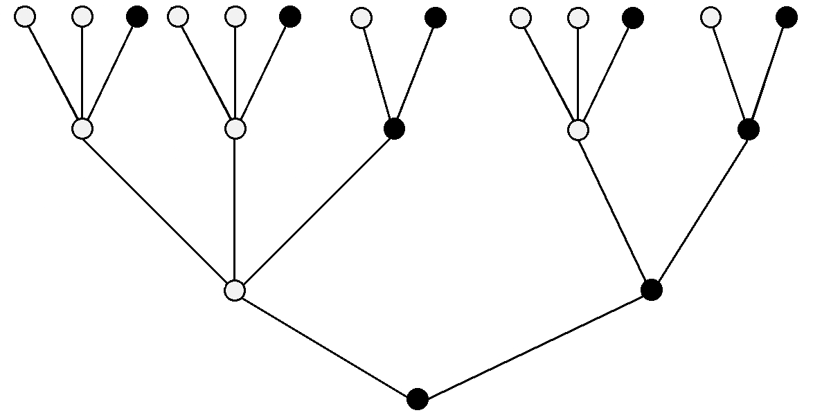
Figure 1. An example of a tree constructed by a substitution matrix.

After we have introduced the graphs in question, we will now come to the associated operators. Given a tree ${\mathbb{T}}={\mathbb{T}}(M,j)$ as above with vertex set $V$ we consider the Hilbert space

$$\ell^{2}({\mathbb{T}}):=\ell^{2}(V):=\{f:V\longrightarrow{\mathbb{C}}:\sum_{v\in V}|f(v)|^{2}<\infty\}$$

with inner product given by

$$\langle f,g\rangle=\sum_{v\in V}\overline{f(v)}g(v).$$

In our context the analogue of the usual Laplacian in the Euclidean situation will be given by the adjacency matrix

$$L:\ell^{2}({\mathbb{T}})\longrightarrow\ell^{2}({\mathbb{T}})$$

$$(L\varphi)(x)=\sum_{y\sim x}\varphi(y).$$

The operator $L$ can easily be seen to be bounded (as the vertex degree is uniformly bounded). Moreover, the operator $L$ is clearly symmetric. Hence, $L$ is a selfadjoint operator. We will be interested in the spectral theory of $L$ and later of (random) perturbations of it.

Remark. Various extension of the operator $L$ can be treated by our methods. We could, for example, include edge weights and / or potentials depending only on the labeling. Also, it is possible to replace the underlying (constant) measure on the set of vertices by any label invariant measure. Specifically, all our results below remain valid for the operator

$$\Delta:=\mbox{I }-D^{-1}L$$

on the weighted $\ell^{2}$ space $\ell^{2}(V,D)$. Here, $I$ is the identity and $D$ is the operator of multiplication with the degree. This operator is sometimes known as normalized Laplacian. It is a selfadjoint operator and occurs in the investigation of random walks (see below). We refrain from further discussing this here in order to simplify the presentation, see [Kel2] for details.

3. Why study trees of finite cone type?

In this section we provide some background on trees of finite cone type. In particular, we discuss the following three contexts in which these graphs and their associated operators came up.

1. Random operators on trees.

2. Simplified models of regular tessellations of the hyperbolic plane.

3. Random walks on trees.

3.1. Random operators on trees

After the seminal work of the theoretical physicist Anderson on random media in the 50ies, the mathematically rigorous investigation of random operators gained momentum in the 70ies beginning with work due to mainly Pastur, Molchanov, Goldshtein. A main focus of the investigations is the phenomenon of localization, i.e., intervals with pure point spectrum with exponentially decaying eigenfunctions. In the one-dimensional situation a most general result of Carmona / Klein / Martinelli [CKM] shows localization on the whole spectrum. For the treatment of models in arbitrary dimensions key results were provided by the works of Fröhlich / Spencer [FS] and Fröhlich / Martinelli / Scoppola / Spencer, and von Dreyfuss / Klein [vDK]. This lead to an approach called multi-scale analysis. This was later complemented by a different approach known as Aizenman-Molchanov method [AM]. Building on these approaches a large body of work has accumulated over the last three decades and it seems fair to say that localization is quite well understood by now.

The big open question now concerns ’existence of extended states’, i.e., the occurrence of an absolutely continuous component in the spectrum. For one dimensional models such a component is known to be absent. In fact, the spectrum is known to be pure point (see above). In two dimensional models the behavior expected by physicists is under dispute. But for higher dimensions, i.e., from dimension 3 on, the occurrence of an absolutely continuous component in the spectrum of a random model is conjectured to take place. So far, this could not be proven.

On the other hand, work of Klein [Kle, Kle2] in the 90ies showed that an absolutely continuous component exists in a perturbative regime for infinite dimensional random models, i.e., for models on trees. So, random models on trees are the only models among the ’usual’ random operators where the extended states conjecture is proved. Various groups have taken up this line of investigation. In fact, both [ASW] and [FHS, FHS2] come up with alternative approaches at about the same time.

Beyond the perturbative regime, some surprises have been discovered concerning the regime of extended states on regular trees. Among them is that even at weak disorder, the extended states can be found well beyond energies of the unperturbed model into the regime of Lifshitz tails. The mechanism for the appearance of extended states in this non-perturbative regime are disorder-induced resonances [AW].

All these works deal with regular trees. This restriction to regular trees is rather by convenience than by intrinsic (physical) reasons. Thus, it is reasonable to consider more complicated models. In fact, the authors of the present article started their corresponding investigations with an attempt to study spectral theory of regular tessellations of the hyperbolic plane. The tessellation models turned out to be too hard to analyze due to the appearance of loops in the graphs. Then, systematic ways of cutting loops lead us to models of trees of finite cone type (compare [Kel2] for details), see Figure 2 from [Kel1].

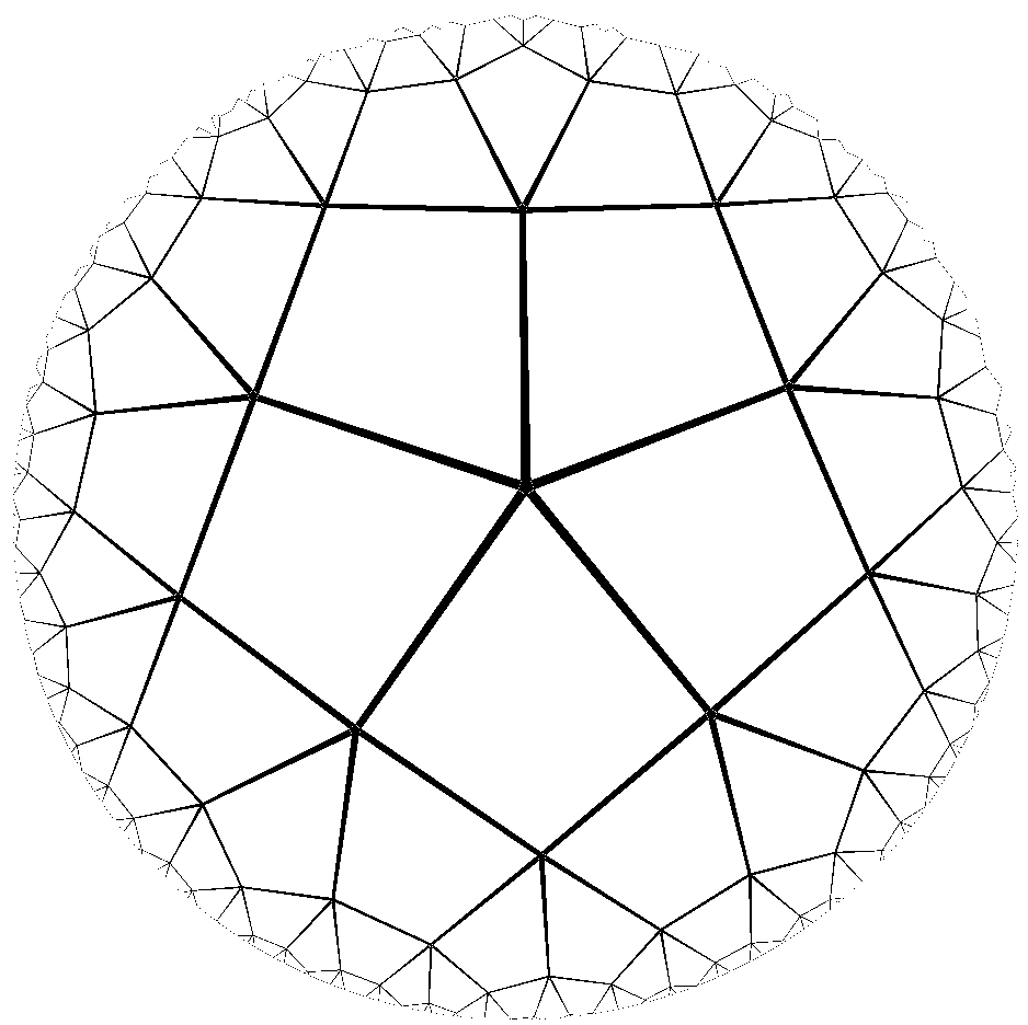
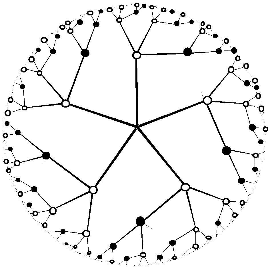
Figure 2. The regular hyperbolic (4,5)-tessellation and a spanning tree which is constructed by a substitution matrix.

A similar occurrence of trees of finite cone type in the spectral theory of regular tessellations of the hyperbolic plane will be discussed below.

As for recent works on various variants of trees we also mention [FHS3, FHH, Hal, KS, Sha]

3.2. Regular tilings of the hyperbolic plane

Trees of finite cone type have also come up in the study of spectral theory of tilings of the hyperbolic plane. This will be discussed in this section.

The three basic models of planar geometry are the Euclidean plane (with curvature zero), the sphere (with curvature 1) and the hyperbolic plane (with curvature $-1$). Each of these three models allows for regular tessellations and the spectral theory of the (discrete) Laplacians associated to these tessellations has been quite a focus of research. Concerning this spectral theory of regular tessellations the basic picture is as follows:

• Euclidean plane: band spectrum, purely absolutely continuous spectrum.

• Sphere in three dimensional Euclidean space: finite pure point spectrum

• Hyperbolic plane: quite unknown!

Let us comment on the last point. Spectral theory may be divided into investigation of the form of the spectrum and investigation of the type of the spectrum. For both parts only some pieces of information are known for regular tessellations of the hyperbolic plane.

Quite some effort has been put into studying the infimum of the spectrum. It is known that this infimum is positive (due to basic Cheeger estimates). The exact value is unknown. In fact, there is a famous conjecture of Sarnak stating that the infimum of the spectrum is an algebraic number (see the book [Woe] of Woess for discussion). While the conjecture is open, some works have been devoted to giving estimates on the actual value of the infimum of the spectrum. Among these we mention [BCCSH, BCS, CV, Nag, Zuk]. In particular, the best lower bounds known so far is established by Nagnibeda in [Nag] and the best upper bound by Bartholdi / Ceccherini-Silberstein in [BCS]. Quite remarkably these bounds agree up to the third digit. In a very recent preprint, the upper bounds of [BCS] seem to have been improved once more by Gouezel in [Gou]. (Note that these works use a somewhat different normalization and thus their use of lower and upper bound is just the reverse of our use here.)

In our context the mentioned work of Nagnibeda is most relevant. In fact, her approach to the lower bound can be divided in three steps: In the first step she associates a tree of finite cone type to a given tessellation. This tree arises as some sort of universal covering of the tessellation. In the second step she shows that the infimum of the spectrum of the tessellation can be bounded below by the infimum of the spectrum of the tree. In the last step she then bounds the spectrum of the tree. So, trees of finite cone type most naturally come up in the study of spectral theory of regular tessellations.

As for further results on spectral theory it seems that for those regular tessellations of the hyperbolic plane which are Cayley graphs of torsion free groups some information on both parts of spectral theory is available. More specifically, after talking with various experts it seems to us that for such models there should be no eigenvalues as a consequence of (an established version of) Linnells zero-divisor conjecture and that the spectrum should be an interval as a consequence of (an established version of) Baum-Connes conjecture. It is unclear (to us at least) whether explicit statements to these effects can be found in the literature. In any case, no information on existence of absolutely continuous spectrum for such models seems available at the moment.

For those regular tessellations of the hyperbolic plane which are not Cayley graphs of torsion free subgroups even less is known. It is tempting to think of these models as certain forms of coverings of a torsion free situation. This suggests that they have bands of absolutely continuous spectrum and possibly finitely many eigenvalues in between the bands. The extend to which such a reasoning could be made precise is unclear at the moment. Two of the authors of the present paper (M.K. and D.L.) are currently working together with Lukasz Grabowski on this topic, [GKL].

Remark. To us it seems most remarkable that so little is known on spectral types of (discrete) Laplacians on regular tessellation of the hyperbolic plane. This is somewhat reminiscent of the situation encountered in the study of quasicrystals. There essentially nothing is known on the spectral type of such basic models as Laplacian associated to Penrose tiling. In both cases once encounters very natural geometric situations exhibiting a large degree of overall order. Still it seems hard to get a grip on. On the technical level this seems to be related to the lack of suitable Fourier type analysis.

3.3. Random walk on trees of finite cone type

Trees of finite cone type have also been studied in the context of random walks. This will be briefly discussed in this section.

Let ${\mathbb{T}}$ be tree of finite cone type and denote the operator of multiplication by the degree by $D$. Then, $P=D^{-1}L=I-\Delta$ is a selfadjoint operator on the Hilbert space with the vertex degree as a measure. It can be seen as the transition matrix of a random walk (in discrete time). Properties of this random walk have been studied in particular in [Lyo, Tak, NW, Mai]. These works are mostly concerned with recurrence and transience, i.e., – very roughly speaking – the behavior of the Greens function at the infimum of the spectrum.

4. Which spectral properties have trees of finite cone type?

In this section we present some results on spectral theory of trees of finite cone type.

To be specific we will consider the following situation: $\mathcal{A}$ is the set of vertex labels, $M:\mathcal{A}\times\mathcal{A}\longrightarrow{\mathbb{N}}_{0}$ is the substitution matrix and the tree ${\mathbb{T}}={\mathbb{T}}(M,j)$ with root labeled by $j$ is generated according to the rule given above that every vertex with label $k$ of the $n$-th sphere is joined to $M_{l,k}$ vertices of label $l$ of the $(n+1)$-sphere. Moreover, we will assume that the assumptions (M0), (M1) and (M2) are in effect. We will then consider the operator $L:\ell^{2}({\mathbb{T}})\longrightarrow\ell^{2}({\mathbb{T}})$, $(L\varphi)(x)=\sum_{y\sim x}\varphi(y)$ introduced above.

4.1. The unperturbed operator

In this section we present the basic result on the spectral theory of the unperturbed operator.

Theorem 1 ([KLW]).

There exist finitely many intervals such that for every $j\in\mathcal{A}$ the spectrum of $L$ associated to ${\mathbb{T}}(M,j)$ consists of exactly these intervals and is purely absolutely continuous.

Remarks. (a) There is an effective bound on the number of bands by results of Milnor [Mil] on algebraic varieties.

(b) A tree constructed from $M$ not satisfying $M_{j,j}>0$ may have eigenvalues.

(c) The result generalizes the well-known spectral theory of regular trees.

4.2. Radially symmetric perturbations

A function $v$ on the vertices is radially labeling symmetric if vertices with the same label in the same generation yield the same value.

Theorem 2 ([KLW]).

Assume ${\mathbb{T}}$ is not a regular tree. Then, for every compact $I$ contained in the interior of $\sigma(L)\setminus\{0\}$, there exists $\lambda>0$ such that for all radially labeling symmetric $v$ with values in $[-1,1]$ we have

$$I\subset\sigma_{ac}(L+\lambda v)\>\;\mbox{and}\>\;I\cap\sigma_{sing}(L+\lambda v)=\emptyset.$$

Remarks. The corresponding statement is quite invalid for regular trees. There one is essentially in a one-dimensional situation (see e.g. [Bre]) and then a random potential yields pure point spectrum. This is already discussed in [ASW] (see [BF] as well for related material).

Corollary ([KLW]).

Assume ${\mathbb{T}}$ is not a regular tree. Then, for every radially labeling symmetric $v$ with $v(x)\to 0$ for $x\to\infty$, we have

$$\sigma_{ac}(L)=\sigma_{ac}(L+v).$$

Remark. For regular trees one is far from having such a general statement compare e.g. [Kup].

4.3. Random perturbations

Here, we consider random perturbations of our model. Thus, beyond the operator $L$ as above we are given the following pieces of data:

A probability space $(\varOmega,{\mathbb{P}})$ and a measurable map

$$(v,\vartheta):\varOmega\times V\longrightarrow(-1,1)\times(-1,1),\>\;(\omega,x)\mapsto(v_{x}^{\omega},\vartheta_{x}^{\omega})$$

satisfying the following two properties:

• For all $x,y\in V$ the random variables $(v_{x},\vartheta_{x})$ and $(v_{y},\vartheta_{y})$ are independent if the forward trees of $x$ and $y$ do not intersect.

• For all $x,y\in V$ that share the same label the restrictions of the random variables $(v,\vartheta)$ to the isomorphic forward trees of $x$ and $y$ are identically distributed.

For a vertex $x$ that is not the root let $\dot{x}$ be the vertex such that $x$ is a forward neighbor of $\dot{x}$ and denote

$$\vartheta_{x,\dot{x}}=\vartheta_{\dot{x},x}=\vartheta_{x}.$$

We then consider the operator

$$(H^{\lambda,\omega}\varphi)(x)=\sum_{y\sim x}(\varphi(y)+\lambda\vartheta^{\omega}_{x,y}\varphi(y))+\lambda v_{x}^{\omega}\varphi(x).$$

Theorem 3.

There exists a finite set $\Sigma_{0}\subset\sigma(L)$ such that for each compact $I\subset\sigma(L)\setminus\Sigma_{0}$ there is $\lambda>0$ such that $H^{\lambda,\omega}$ has almost surely purely absolutely continuous spectrum in $I$ for all $(v,\vartheta)$ satisfying the conditions above.

Remarks. (a) The theorem includes regular trees as a special case.

(b) If the tree is not regular (and in some other cases as well), $\Sigma_{0}$ is just the set of boundary bounds of $\sigma(L)$ together with $0$.

5. How are trees of finite cone type related to multi-type Galton Watson trees?

In this section we relate trees of finite cone type to multi-type Galton Watson trees. We present a result stating that whenever certain Galton Watson trees are close to a tree of finite cone type in distribution, then these random trees inherit some of the absolutely continuous spectrum from the tree of finite cone type. The operators on such trees are also random operators, where now the randomness is induced by the underlying combinatorial geometry rather than by a random perturbation of the parameters.

A multi-type Galton Watson branching process $b$ with finite set ${\mathcal{A}}$ of types or labels is determined by numbers $P_{ij}^{(b)}(n)$ such that $\sum_{n=0}^{\infty}P_{ij}^{(b)}(n)=1$, $i,j\in{\mathcal{A}}$. The number $P_{ij}(n)$ encodes the probability that a vertex with label $i$ has $n$ forward neighbors of label $j$. We may encode the possible configurations of forward neighbors of a vertex by vectors $s\in{\mathbb{N}}_{0}^{{\mathcal{A}}}$ (i.e., the vertex has $s_{j}$ forward neighbors of type $j$) and define by

$${\mathbb{P}}_{i}^{(b)}(s)=\sum_{j\in{\mathcal{A}}}P_{ij}^{(b)}(n)$$

the probability that a vertex of type $i\in{\mathcal{A}}$ has the forward configuration $s$. Moreover, $\|s\|_{1}=\sum_{j\in A}s_{j}$ denotes the total number of forward neighbors of a configuration $s$.

We impose two further assumptions on the branching processes. The first is a mild growth condition and the second says that every vertex has at least one forward neighbor:

• There is $p>1$ such that $\sum_{s\in{\mathbb{N}}_{0}^{{\mathcal{A}}}}{\mathbb{P}}^{(b)}_{j}(s)\|s\|_{1}^{p}<\infty$ for all $j\in{\mathcal{A}}$.

• ${\mathbb{P}}^{(b)}_{j}(0)=0$ for all $j\in{\mathcal{A}}$.

We observe that a tree of finite cone type given by a labeling set ${\mathcal{A}}$ and a substitution matrix $M$ can be viewed as such a multi-type Galton Watson branching process $b_{M}$ by letting $P_{ij}^{b_{M}}(n)=1$ for $n=M_{i,j}$ and $0$ otherwise. Hence,

$${\mathbb{P}}^{(b_{M})}_{i}(M_{i,\cdot})=1\quad\mbox{and}\quad{\mathbb{P}}^{(b_{M})}_{i}(s)=0\mbox{ for $s\neq M_{i,\cdot}$}.$$

Obviously, (B1) is satisfied and (B2) follows from (M1). In this sense, trees of finite cone type are multi-type Galton Watson trees with deterministic distribution.

We introduce a metric $d_{p}$ on branching processes with the same type set ${\mathcal{A}}$ that satisfy (B1) for the same $p>1$ via

$$d_{p}(b_{1},b_{2})=\max_{i\in{\mathcal{A}}}\sum_{s\in{\mathbb{N}}_{0}^{{\mathcal{A}}}}|{\mathbb{P}}_{i}^{(b_{1})}(s)-{\mathbb{P}}_{i}^{(b_{2})}(s)|\|s\|_{1}^{p}.$$

We denote the set of realizations of a Galton Watson branching process by $\Theta(b)$. For $\theta=(V^{\theta},E^{\theta})\in\Theta(b)$ we denote the adjacency matrix on $\ell^{2}(\theta)=\ell^{2}(V^{\theta})$ by $L^{\theta}$. The operator $L^{\theta}$ may not be bounded, but by techniques of [GS] its restrictions to the functions of finite support is almost sure essentially selfadjoint on $\ell^{2}(\theta)$.

Given a fixed tree of finite cone type ${\mathbb{T}}$ we can now state a theorem proven in [Kel2]. Loosely speaking it says that operators $L^{\theta}$ on random trees $\theta$ close to ${\mathbb{T}}$ in distribution inherit almost surely some of the absolutely continuous spectrum of $L$.

Theorem 4.

There exists a finite set $\Sigma_{0}\subset\sigma(L)$ such that for each compact $I\subset\sigma(L)\setminus\Sigma_{0}$ there is $\lambda$ such that if a multi-type Galton Watson branching process $b$ satisfies (B1), (B2) and

$$d_{p}(b,b_{M})<{\lambda},$$

then $L^{\theta}$ has purely absolutely continuous spectrum in $I$ for almost all $\theta\in\Theta(b)$.

A strategy for a proof of such a theorem for certain single-type Galton Watson trees was also outlined in [FHS3].

6. Some ideas behind the proofs

For a tree ${\mathbb{T}}={\mathbb{T}}(M,j)$, $j\in{\mathcal{A}}$, and a vertex $o$ let ${\mathbb{T}}_{o}$ be the forward tree with root $o$. The forward Green function of an operator $H$, acting as

$$H{\varphi}(x)=\sum_{y\sim x}t_{xy}{\varphi}(y)+v(x){\varphi}(x)$$

on $\ell^{2}({\mathbb{T}})$, at $o$ is defined by

$$\varGamma_{o}(z,H):=\langle(H_{{\mathbb{T}}_{o}}-z)^{-1}\delta_{o},\delta_{o}\rangle,\quad z\in{\mathbb{H}},$$

where ${\mathbb{H}}=\{z\in{\mathbb{C}}\mid\Im z>0\}$. The second resolvent formula gives the recursion formula

$$-\frac{1}{\varGamma_{o}(z,H)}=z-v(o)+\sum_{y\in S_{o}}|t_{oy}|^{2}\varGamma_{y}(z,H),$$

where $S_{o}$ is the forward sphere of $o$.

6.1. The unperturbed operator

We present a basic inequality which shows the absolute continuity of the spectral measure of the unperturbed operator $L$ at the root.

For $H=L$ the forward Green function ${\Gamma}_{x}(z,L)$ is equal for all vertices $x$ with the same label $j$, thus, we write ${\Gamma}_{j}(z,L)$. The recursion formula now reads

$$-\frac{1}{\varGamma_{j}(z,L)}=z+\sum_{k\in{\mathcal{A}}}M_{j,k}\varGamma_{k}(z,L),$$

Taking imaginary parts in the recursion formula and multiplying by $|{\Gamma}_{j}(z,L)|^{2}$, we arrive at

$$\Im{\Gamma}_{j}(z,L)=\sum_{k\in{\mathcal{A}}}{M_{j,k}}\Im{\Gamma}_{k}(z,L)|{\Gamma}_{j}(z,L)|^{2}\geq M_{j,j}\Im{\Gamma}_{j}(z,L)|{\Gamma}_{j}(z,L)|^{2}$$

since ${\Gamma}_{k}(z,L)$ are Herglotz functions and, therefore, $\Im{\Gamma}_{k}(z,L)>0$ for $z\in{\mathbb{H}}$. Hence,

$$|{\Gamma}_{j}(z,L)|\leq{{|M_{j,j}|}^{-\frac{1}{2}}}.$$

This gives that the Green function is uniformly bounded on ${\mathbb{H}}$. By standard results, the spectral measure associated to the delta function of the root must then be absolutely continuous. The result for arbitrary spectral measures follows by further considerations using the recursion formula, confer [KLW, Proposition 3].

6.2. Random operators

In this section we discuss the strategy of the proof of absolutely continuous spectrum for random operators. Consider the function ${\gamma}:{\mathbb{H}}\times{\mathbb{H}}\to[0,\infty)$

$${\gamma}(g,h)=\frac{|g-h|^{2}}{\Im g\Im h},\qquad g,h\in{\mathbb{H}},$$

which is related to the hyperbolic metric $d_{{\mathbb{H}}}$ of the upper half plane viz

$$d_{{\mathbb{H}}}=\cosh^{-1}(\tfrac{1}{2}{\gamma}+1).$$

The function ${\gamma}$ is symmetric and zero only at the diagonal, but it does not satisfy the triangle inequality. Nevertheless, ${\gamma}$ works very well with the recursion formula.

The recursion formula induces a map $\Phi:{\mathbb{H}}^{S_{x}}\to{\mathbb{H}}$

$$(g_{x})_{x\in S_{o}}\mapsto-\frac{1}{z-v(o)+\sum_{x\in S_{o}}g_{x}},$$

mapping $({\Gamma}_{x}(z,H))_{x\in S_{o}}$ to ${\Gamma}_{o}(z,H)$, which decomposes into maps

$$\rho\circ{\sigma}\circ\tau:{\mathbb{H}}^{S_{o}}\longrightarrow{\mathbb{H}}\longrightarrow{\mathbb{H}}\longrightarrow{\mathbb{H}}$$

given by

$$\tau((g_{x}))=\sum_{x\in S_{o}}g_{x},\quad{\sigma}(g)=z-v(o)+g,\quad\rho(g)=-\frac{1}{g}.$$

The map $\Phi$ turns out to be a hyperbolic contraction in a certain sense, e.g. ${\gamma}(\Phi(g),\Phi(h))<\sup_{y\in S_{x}}{\gamma}(g_{y},h_{y})$, $g,h\in{\mathbb{H}}^{S_{o}}$. Indeed, $\rho$ is an isometry and ${\sigma}$ is a uniform contraction, however, ’unfortunately’ with the contraction coefficient going to one as on $\Im z\to 0$. Finally, the map $\tau$ can be seen to be a hyperbolic mean, (i.e., as $g\mapsto|S_{x}|g$ is a hyperbolic isometry we may also consider $\widetilde{\tau}((g_{x}))=\frac{1}{|S_{x}|}\sum_{y}g_{y}$ instead of $\tau$). A hyperbolic mean may contract the input values for two reasons: either two of the vectors $g_{x}-h_{x}$, $x\in S_{o}$, are linearly independent or two of the quantities $|g_{x}-h_{x}|/\Im g_{x}\Im h_{x}$, $x\in S_{o}$ are different. This is exploited in the proof.

We further use that the random variables ${\Gamma}_{x}(z,H^{{\lambda},\omega})$, are independent for $x\in S_{o}$, and identically distributed for all $x$ with the same label. Consequently, we introduce the random variables $G:\Omega\to[0,\infty)^{{\mathcal{A}}}$

$$G_{j}={\gamma}({\Gamma}_{x}(z,H^{{\lambda},\omega}),{\Gamma}_{x}(z,L))^{p}$$

for some $p>1$ and $x$ having the label $j$.

The crucial estimate is then the following vector inequality. We show that there are ${\delta}>0$, a stochastic $(|{\mathcal{A}}|\times|{\mathcal{A}}|)$ matrix $P$ and $C$ such that

$${\mathbb{E}}(G)\leq(1-{\delta})P{\mathbb{E}}(G)+C,$$

where the inequality is of course interpreted componentwise.

By the Perron-Frobenius theorem there is a positive left eigenvector $u$ of $P$ and we arrive at

$$\langle u,G\rangle\leq(1-{\delta})\langle u,PG\rangle+C=(1-{\delta})\langle u,G\rangle+C$$

and, hence,

$${\mathbb{E}}({\gamma}({\Gamma}_{x}(z,H^{{\lambda},\omega}),{\Gamma}_{x}(z,L))^{p})={\mathbb{E}}(G_{j})\leq\frac{C}{{\delta}u_{j}}$$

for all $x$ where $j$ is the label of $x$.

By standard arguments found in [Kle2], [FHS2] and [Kel1, KLW2], one deduces

$$\liminf_{\eta\to 0}\int_{I}|\langle(H^{{\lambda},\omega}-E-i\eta)^{-1}{\delta}_{x},{\delta}_{x}\rangle|^{p}dE<\infty$$

almost surely. This, however, yields purely absolutely continuous spectrum in $I$ by a limiting absorption principle, see [Kle2].

At the end we indicate how the proof for Galton Watson trees fits in the scheme above. For realizations $\theta\in\Theta(b)$. The probability that the first two spheres in $\theta$ look exactly like the ones of the tree of finite cone type is very large by the assumption $d_{p}(b,b_{M})<{\lambda}$.

To prove the crucial vector inequality above, we divide the expected value in the ’good part’, where the spheres are exactly the same as in the deterministic case, and the ’other part’. It turns out that the error made in the ’other part’ is bounded which is then swallowed by the small probability of its occurrence. For the ’good part’ we apply the proof for random potentials above to conclude the statement.

References

- [AM] M. Aizenman, S. Molchanov, Localization at large disorder and at extreme energies: an elementary derivation, Comm. Math. Phys. 157 (1993), 2, 245–278.
- [ASW] M. Aizenman, R. Sims, S. Warzel, Stability of the absolutely continuous spectrum of random Schrödinger operators on tree graphs, Probab. Theory Related Fields 136 (2006), 363–394.
- [AW] M. Aizenman, S. Warzel, Resonant delocalization for random Schrödinger operators on tree graphs, J. Eur. Math. Soc. (JEMS) 15 (2013), 1167- 1222
- [BCS] L. Bartholdi, T. Ceccherini-Silberstein, Growth series and random walks on some hyperbolic graphs, Monatsh. Math. 136 (2002), 181–202.
- [BCCSH] L. Bartholdi, S. Cantat, T. Ceccherini-Silberstein, P. de la Harpe, Estimates for simple random walks on fundamental groups of surfaces, Colloq. Math. 72 (1997), 173 -193.
- [Bre] J. Breuer, Singular continuous spectrum for the Laplacian on certain sparse trees, Commun.Math. Phys. (2007), 269, 851–857.
- [BF] J. Breuer, R. L. Frank, Singular spectrum for radial trees, Rev. Math. Phys. 21 (2009), no. 7, 1–17.
- [CKM] R. Carmona, A. Klein, F. Martinelli, Anderson localization for Bernoulli and other singular potentials, Comm. Math. Phys. 108 (1987), 41–66
- [CV] P.-A. Cherix, A. Valette, On spectra of simple random walks on one-relator groups, with an appendix by Paul Jolissaint. Pacific J. Math. 175 (1996), 417 -438.
- [vDK] H. von Dreifus, A. Klein, A new proof of localization in the Anderson tight binding model, Comm. Math. Phys. 124 (1989), 285 -299.
- [FS] J. Fröhlich, T. Spencer, Absence of diffusion in the Anderson tight binding model for large disorder or low energy, Comm. Math. Phys. 88 (1983), 151 -184.
- [FMSS] J. Fröhlich , F. Martinelli , E. Scoppola and T. Spencer, Constructive proof of localization in the Anderson tight binding model, Comm. Math. Phys. 101 (1985), 21 -46.
- [FHH] R. Froese, F. Halasan, D. Hasler, Absolutely continuous spectrum for the Anderson model on a product of a tree with a finite graph, J. Funct. Anal. 262 (2012), 1011 -1042.
- [FHS2] R. Froese, D. Hasler, W. Spitzer, Absolutely continuous spectrum for the Anderson model on a tree: A geometric proof of Kleins theorem, Commun. Math. Phys. 269 (2007), 239–257.
- [FHS3] R. Froese, D. Hasler, W. Spitzer, Absolutely continuous spectrum for a random potential on a tree with strong transverse correlations and large weighted loops, Rev. Math. Phys. 21 (2009), 709 -733.
- [FHS] R. Froese, D. Hasler, W. Spitzer, Transfer matrices, hyperbolic geometry and absolutely continuous spectrum for some discrete Schrödinger operators on graphs, J. Funct. Anal. 230 (2006), 184–221.
- [GKL] L. Grabowski, M. Keller, D. Lenz, in preparation.
- [GS] S. Golénia, C. Schumacher, The problem of deficiency indices for discrete Schrödinger operators on locally finite graphs, J. Math. Phys. 52 (2011).
- [Gou] S. Gouezel, A numerical lower bound for the spectral radius of random walks on surface groups, Preprint 2013, arXiv:1310.4265.
- [Hal] F. Halasan, Absolutely continuous spectrum for the Anderson model on some tree-like graphs, Ann. Henri Poincaré 13 (2012), 789 -811.
- [KLW] M. Keller, D. Lenz, S. Warzel, On the spectral theory of trees with finite cone type, Israel Journal of Mathematics, 194, (2013), 107–135.
- [KLW2] M. Keller, D. Lenz, S. Warzel, Absolutely continuous spectrum for random operators on trees of finite cone type, Journal d’Analyse Mathematique, 118 (2012), 363-396.
- [Kel1] M. Keller, On the spectral theory of operators on trees, PH D Thesis, 2010.
- [Kel2] M. Keller, Absolutely continuous spectrum for multi-type Galton Watson trees, Annales Henri Poincaré, 13, (2012), 1745–1766.
- [Kle] A. Klein, Absolutely continuous spectrum in the Anderson model on the Bethe lattice. Math. Res. Lett. 1 (1994), 399–407.
- [Kle2] A. Klein, Extended states in the Anderson model on the Bethe lattice, Adv. Math. 133 (1998), 163–184.
- [KS] A. Klein, C. Sadel, Absolutely continuous spectrum for random Schrödinger operators on the Bethe strip, Math. Nachr. 285 (2012), 5–26.
- [Kup] S. Kupin, Absolutely continuous spectrum of a Schrödinger operator on a tree, J. Math. Phys. 49 (2008), 113506.
- [Lyo] R. Lyons, Random walks and percolation on trees, Ann. Probab. 18 (1990), 931–958.
- [Mai] J. Mairesse, Random walks on groups and Monoids with a harmonic Markovian measure, Electron. J. Probab. 10 (2005), 1417–1441.
- [Mil] J. Milnor, On the Betti numbers of real varieties, Proc. Amer. Math. Soc. 15 (1964) 275–280.
- [Nag] T. Nagnibeda, An upper bound for the spectral radius of a random walk on surface groups Zap. Nauchn. Sem. S.-Peterburg. Otdel. Mat. Inst. Steklov. (POMI) 240 (1997), J. Math. Sci. (New York) 96 (1999), no. 5, 3542–3549.
- [NW] T. Nagnibeda, W. Woess, Random walks on trees with finite cone type, J. Theoret. Probab. 15 (2002), 383–422.
- [Sad] C. Sadel, Absolutely continuous spectrum for random Schrödinger operators on tree-strips of finite cone type, Ann. Henri Poincaré 14 (2013), 737-773.
- [Sha] M. Shamis, Resonant delocalization on the Bethe strip, Annales Henri Poincaré (2013), 1-19.
- [Tak] C. Takacs, Random walk on periodic trees, Electron. J. Probab. 2 (1997), 1–16.
- [Woe] W. Woess, Random walks on infinite graphs and groups. Cambridge Tracts in Mathematics, 138. Cambridge University Press, Cambridge, 2000. xii+334 pp
- [Zuk] A. Zuk, A remark on the norm of a random walk on surface groups, Colloq. Math. 72 (1997), 195–206.