Anisotropic quantum scattering in two dimensions

Abstract

We study the quantum scattering in two spatial dimensions (2D) without the usual partial-wave formalism. The analysis beyond the partial-wave approximation allows a quantitative treatment of the anisotropic scattering with a strong coupling of different angular momenta nonvanishing even at the zero-energy limit. High efficiency of our method is demonstrated for the 2D scattering on the cylindrical potential with the elliptical base and dipole-dipole collisions in the plane. We reproduce the result for the 2D scattering of polarized dipoles in binary collisions obtained recently by Ticknor [Phys. Rev. A 84, 032702 (2011)] and explore the 2D collisions of unpolarized dipoles.

I Introduction

In recent years, the problem of anisotropic quantum scattering in two spatial dimensions (2D) attracts increasing interest. It is stimulated by the spectacular proposals for prospects to create exotic and highly correlated quantum systems with dipolar gases ref1 ; ref2 . Particularly, there were considered anisotropic superfluidity ref3 , 2D dipolar fermions ref4 , and few-body dipolar complexes ref5 . The recent experimental production of ultracold polar molecules in the confined geometry of optical traps ref6 ; ref7 ; ref8 has opened up ways to realize these phenomena. Noteworthy also is a rather long history of research of 2D quantum effects in condensed matter physics. One can note superfluid films ref9 , high-temperature superconductivity ref10 , 2D materials, such as graphene ref11 , and even possibilities for topological quantum computation ref12 . Unique opportunities for modeling these 2D effects in a highly controlled environment have recently appeared with the development of experimental techniques for creating quasi-2D Bose and Fermi ultracold gases ref13 .

Interest in the processes and effects in 2D-geometry has stimulated the theory of elementary quantum two-body systems and processes in the plane. Special consideration should be given to the anisotropy and long-range character of the dipole-dipole interaction. Actually, usual partial-wave analysis becomes inefficient for describing the dipole-dipole scattering due to the strong anisotropic coupling of different partial-waves in the asymptotic region ref14 ; ref15 . Recently, considerable progress in the analysis of the 2D and quasi-2D (q2D) scattering of dipoles has been achieved ref16 ; ref17 ; ref18 ; ref19 ; ref20 . Thus, the 2D dipolar scattering in the threshold and semiclassical regimes was studied in the case of the dipole polarization directed orthogonally to the scattering plane ref16 . An arbitrary angle of polarization was considered in ref17 .

In this work, we develop a method for quantitative analysis of the 2D quantum scattering on a long-range strongly anisotropic scatterer. Particularly, it permits the description of the 2D collisions of unpolarized dipoles. Our approach is based on the method suggested in ref21 for the few-dimensional scattering which was successfully applied to the dipole-dipole scattering induced by an elliptically polarized laser field in the 3D free-space ref15 .

The key elements of the method are described in Section II. In Section III, we apply the method to the 2D scattering on the cylindrical potential with the elliptical base and the 2D dipole-dipole scattering of unpolarized dipoles. We reproduce the threshold formula ref22b ; ref24 for the scattering amplitude on the cylinder potential with the circular base and the results of ref16 ; ref17 for the 2D scattering of polarized dipoles. High efficiency of the method has been found in all problems being considered. The last Section contains the concluding remarks. Some important details of the computational scheme and illustration of the convergence are given in Appendices.

II 2D Scattering problem in angular-grid representation

The quantum scattering on the anisotropic potential $U(\rho,\phi)$ in the plane is described by the 2D Schrödinger equation in polar coordinates $(\rho,\phi)$

$$H(\rho,\phi)\Psi\left({\rho,\phi}\right)=E\Psi\left({\rho,\phi}\right)$$ (1)

with the scattering boundary conditions

$$\Psi\left({\rho,\phi}\right)\to e^{i{\bm{q}}\bm{\rho}}+f\left({q,\phi,\phi_{q}}\right)\frac{e^{iq\rho}}{\sqrt{-i\rho}}$$ (2)

in the asymptotic region $\rho\to\infty$ and the Hamiltonian of the system

$$H(\rho,\phi)=-\frac{\hbar^{2}}{2\mu}\left({\frac{1}{\rho}\frac{\partial}{\partial\rho}\left({\rho\frac{\partial}{\partial\rho}}\right)+\frac{1}{\rho^{2}}h^{(0)}(\phi)}\right)+U\left({\rho,\phi}\right).$$

The unknown wave function $\Psi\left({\rho,\phi}\right)$ and the scattering amplitude $f\left({q,\phi,\phi_{q}}\right)$ are searched for the fixed momentum ${\bm{q}}$ defined by the colliding energy $E$ ($q=\sqrt{2\mu E}/\hbar)$ and the direction ${\bm{q}}/q$ of the incident wave (defined by the angle $\phi_{q})$ and for the scattering angle $\phi$ . Here $\mu$ is the reduced mass of the system. In the polar coordinates, the angular part of the kinetic energy operator in $H(\rho,\phi)$ has a simple form $h^{(0)}(\phi)=\frac{\partial^{2}}{\partial\phi^{2}}$. The interaction potential $U\left({\rho,\phi}\right)$ can be anisotropic in the general case, i.e. to be strongly dependent on $\phi$. It is clear that varying the direction of the incident wave ${\bm{q}}/q$ can be replaced by the rotation $U\left({\rho,\phi}\right)\to U\left({\rho,\phi+\phi_{q}}\right)$ of the interaction potential by the angle $\phi_{q}$ for the fixed direction of the incident wave, which we choose to be coincident with the x-axis. Thus, in the case of anisotropic potential $U\left({\rho,\phi}\right)$ the task is to solve the problem (1) with the interaction potential $U\left({\rho,\phi+\phi_{q}}\right)$ for all possible $\phi_{q}$ and fixed $E$ with the scattering boundary conditions

$$\Psi\left({\rho,\phi}\right)\to\exp\{iq\rho\cos(\phi)\}+f\left({q,\phi,\phi_{q}}\right)\frac{e^{iq\rho}}{\sqrt{-i\rho}}\,.$$ (3)

If the scattering amplitude $f\left({q,\phi,\phi_{q}}\right)$ is found, one can calculate the differential scattering cross section

$${d\sigma(q,\phi,\phi_{q})}\mathord{\left/{\vphantom{{d\sigma(q,\Omega)}{d\Omega}}}\right.\kern-1.2pt}{d\Omega}\mbox{=}{\left|{f(q,\phi,\phi_{q})}\right|^{2}}\,,$$ (4)

where $d\Omega=d\phi d\phi_{q}$, as well as the total cross section

$$\sigma(q)\mbox{=}\frac{1}{2\pi}\int\limits_{0}^{2\pi}\int\limits_{0}^{2\pi}{\frac{d\sigma}{d\Omega}}d\phi_{q}d\phi$$ (5)

by averaging over all possible orientations $\phi_{q}$ of the scatterer and integration over the scattering angle $\phi$.

To integrate the problem (1),(2), we use the method suggested in ref21 to solving a few-dimensional scattering problem and applied in ref15 for the dipole-dipole scattering in the 3D free-space. Following the ideas of these works we choose the eigenfunctions

$$\xi_{m}(\phi)=\frac{1}{\sqrt{2\pi}}e^{im\left({\phi-\pi}\right)}=\frac{(-1)^{m}}{\sqrt{2\pi}}e^{im\phi}$$ (6)

of the operator $h^{(0)}(\phi)$ as a Fourier basis for the angular-grid representation of the searched wave-function $\Psi\left({\rho,\phi}\right)$. We introduce the uniform grid $\phi_{j}=\frac{2\pi j}{2M+1}\mbox{ }(\mbox{where }j=0,1,...,2M$) over the $\phi$ and $\phi_{q}$-variables and search the wave function as expansion

$$\begin{array}[]{l}\Psi(\rho,\phi)=\frac{1}{\sqrt{\rho}}\sum\limits_{j=0}^{2M}{\sum\limits_{m=-M}^{M}{\xi_{m}(\phi)\xi_{mj}^{-1}\psi_{j}(\rho)}}=\\ =\frac{2\pi}{\sqrt{\rho}}\left({\frac{1}{2M+1}}\right)\sum\limits_{j=0}^{2M}{\sum\limits_{m=-M}^{M}{e^{im(\phi-\phi_{j})}\psi_{j}(\rho)}}\,,\\ \end{array}$$ (7)

where $\xi_{mj}^{-1}=\frac{2\pi}{2M+1}\xi_{jm}^{\ast}=\frac{2\pi}{2M+1}e^{-im\phi_{j}}$ is the inverse matrix to the $\left({2M+1}\right)\times\left({2M+1}\right)$ square matrix $\xi_{jm}=\xi_{m}(\phi_{j})$ defined on the angular grid.

In the representation (7) the unknown coefficients $\psi_{j}(\rho)$ are defined by the values of the searched wave function on the angular grid $\psi_{j}(\rho)=\sqrt{\rho}\Psi(\rho,\phi_{j})$, any local interaction is diagonal

$$\begin{array}[]{lr}U(\rho,\phi)\Psi(\rho,\phi)\left|{{}_{\phi=\phi_{j}}}\right.=\\ =\frac{2\pi}{(2M+1)\sqrt{\rho}}U(\rho,\phi_{j})\sum\limits_{j^{\prime}=0}^{2M}{\sum\limits_{m=-M}^{M}{e^{im(\phi_{j}-\phi_{j^{\prime}})}\psi_{j^{\prime}}(\rho)}}\\ =\frac{1}{\sqrt{\rho}}U(\rho,\phi_{j})\psi_{j}(\rho)\,,\end{array}$$ (8)

and the angular part $h_{jj^{\prime}}^{(0)}$ of the kinetic energy operator has a simple form

$$\begin{array}[]{l}h^{(0)}(\phi)\Psi(\rho,\phi)\left|{{}_{\phi=\phi_{j}}}\right.=\frac{1}{\sqrt{\rho}}\sum\limits_{j^{\prime}=0}^{2M}{h_{jj^{\prime}}^{(0)}\psi_{j^{\prime}}(\rho)}\\ =-\frac{2\pi}{(2M+1)\sqrt{\rho}}\sum\limits_{j^{\prime}=0}^{2M}({\sum\limits_{m=-M}^{M}{m^{2}e^{im(\phi_{j}-\phi_{j^{\prime}})})\psi_{j^{\prime}}(\rho)}}\,.\end{array}$$ (9)

Note that the presence in the interaction potential of the “nonlocal” angular part (i.e. the integration or differentiation over angular variable) leads to destroying the diagonal structure in (8).

Thus, the 2D Schrödinger equation (1) is reduced in the angular-grid representation (7) to the system of $2M+1$ coupled ordinary differential equations of the second order:

$$\frac{d^{2}\psi_{j}(\rho)}{d\rho^{2}}+\frac{2\mu}{\hbar^{2}}\left({E-U(\rho,\phi_{j})+\frac{\hbar^{2}}{8\mu\rho^{2}}}\right)\psi_{j}(\rho)+$$

$$+\frac{1}{\rho^{2}}\sum\limits_{j^{\prime}}{h_{jj^{\prime}}^{(0)}\psi_{j^{\prime}}(\rho)}=0\,.$$ (10)

Since the wave function $\Psi(\rho,\phi_{j})=\frac{\psi_{j}(\rho)}{\sqrt{\rho}}$ must be finite at the origin $\left({\frac{\psi_{j}(\rho)}{\sqrt{\rho}}\to const}\right)$, the “left-side” boundary condition for the functions $\psi_{j}(\rho)$ reads as

$$\psi_{j}(\rho\to 0)\to const{\sqrt{\rho}}\quad(j=0,1,\ldots,2M)\,.$$ (11)

In the asymptotic region $\rho\to\infty$ the scattering boundary condition (3) accepts the form

$$\frac{2\pi}{\sqrt{\rho}(2M+1)}\sum\limits_{j=0}^{2M}{\sum\limits_{m=-M}^{M}{e^{im(\phi-\phi_{j})}\psi_{j}(\rho)}}=$$

$$=\exp\{iq\rho\cos(\phi)\}+f(q,\phi,\phi_{q})\frac{e^{iq\rho}}{\sqrt{-i\rho}}\,.$$ (12)

By using the Fourier expansion for the plane wave $\exp\{iq\rho\cos(\phi)\}$ and the scattering amplitude $f(q,\phi,\phi_{q})$

$$\exp\{iq\rho\cos(\phi)\}=\sum\limits_{m^{\prime}=-M}^{M}{i^{m^{\prime}}J_{m^{\prime}}(q,\rho)e^{i{m}^{\prime}\phi}}$$ (13)

$$f(q,\phi,\phi_{q})=\frac{1}{\sqrt{2\pi}}\sum\limits_{m^{\prime}=-M}^{M}{f_{m^{\prime}}(\phi_{q})e^{i{m}^{\prime}\phi}}$$ (14)

we eliminate the angular dependence from the asymptotic equation (II) and represent the “right-side” boundary condition for the functions $\psi_{j}(\rho\to\infty)$ in the form

$$\frac{2\pi}{(2M+1)\sqrt{\rho}}\sum\limits_{j=0}^{2M}{e^{-im\phi_{j}}\psi_{j}(\rho)}=i^{m}J_{m}(q\rho)\sqrt{2\pi}+$$

$$+\frac{f_{m}(\phi_{q})}{\sqrt{-i\rho}}e^{iq\rho}\,.$$ (15)

To solve the boundary-value problem (II),(11) and (II), we introduce the grid over the $\rho\mbox{-variable}\quad\{\rho_{n}\}\mbox{ (}n=0,1,\ldots,N\mbox{)}$ and reduce the system of differential equations (II) by using the finite-difference approximation of the sixth order to the system of $(N+1)\times(2M+1)$ algebraic equations

$$\hat{A}{\bm{\psi}}=0$$ (16)

with the band-structure of the matrix $\hat{A}$ with the width $(2M+1)\times 7$ of the band. By using the asymptotic equations (II) in the last two points $\rho_{N-1}$ and $\rho_{N}$ one can eliminate the unknown vector $f_{m}(\phi_{q})$ from equation (II) and rewrite the “right-side” boundary condition in the form

$$\sum\limits_{j^{\prime}}\{{A_{j{j}^{\prime},NN-1}\psi_{{j}^{\prime}}(\rho_{N-1})}+{A_{j{j}^{\prime},NN}\psi_{{j}^{\prime}}(\rho_{N})}\}=$$

$$=F_{j,N}(q,\rho_{N-1},\rho_{N})\,.$$ (17)

Analogously, one can eliminate unknown constant from expression (11) by considering asymptotic equations (11) at the first points $\rho_{0}\,,\rho_{1}$ and $\rho_{1}$. The acquired “left-side” boundary condition reads

$$\psi_{j}(\rho_{0}=0)=0\,\,,$$

$$\sum\limits_{j^{\prime}}\{{A_{j{j}^{\prime},11}\psi_{{j}^{\prime}}(\rho_{1})}+{A_{j{j}^{\prime},12}\psi_{{j}^{\prime}}(\rho_{2})}\}=F_{j,1}(q,\rho_{1},\rho_{2})\,.$$ (18)

Thus, the scattering problem is reduced to the boundary value problem (16-II)

$$\hat{A}{\bm{\psi}}={\bm{F}}\,,$$ (19)

which can be efficiently solved with standard computational techniques such as the sweeping method ref25 or the LU-decomposition ref26 . The detailed structure of the matrix of the coefficients $A_{jj^{\prime},nn^{\prime}}$ is discussed in Appendix A. After the solving of Eq.(19) and finding the wave function $\psi_{j}(\rho)$ the scattering amplitude $f(q,\phi,\phi_{q})$ is constructed according to Eqs.(II) and (14).

III Results and Discussion

III.1 Scattering on anisotropic scatterer

First, we have analyzed the 2D scattering on the cylindrical potential barrier with the elliptical base

$$U(\rho,\phi)=\left\{{{\begin{array}[]{*{20}c}{U_{0},\mbox{ }\rho\leqslant a(\phi)\hfill}\\ {0,\mbox{ }\rho>a(\phi)}\,\,.\hfill\\ \end{array}}}\right.$$ (20)

The case of the circular base $a(\phi)=a_{0}$ was considered in ref22b ; ref24 , where analytic formula for the scattering amplitude

$$f(q)\to-\sqrt{\frac{\pi}{2q}}\frac{1}{\ln\left[{\frac{2}{\gamma qa_{\textrm{2D}}}}\right]+i\frac{\pi}{2}}$$ (21)

was obtained at the zero-energy limit $q\to 0$. Here $\gamma=\exp(C)$ and $C=\mbox{0.577...}$ is the Euler constant. We have analyzed the scattering on the potential barrier with circular base $a(\phi)=a_{0}$ for arbitrary momentum $q$. The results of calculation presented in Figs. 1 and 2 confirm the convergence of the scattering amplitude $f(q,\phi,\phi_{q})$ to the analytical value (21) at $q\rightarrow 0$. In this Subsection all the calculations were performed in the units $\hbar=\mu=1$.

In the limiting case of the infinitely high potential barrier (20) with the circular base $a(\phi)=a_{0}$ the asymptotic formula (21) becomes exact for arbitrary $q$. This is confirmed by investigation presented in Table 1 which illustrates the convergence of the numerical values $f(q,\phi,\phi_{q})$ with increasing ($U_{0}\to\infty$) and narrowing ($a_{0}\to 0$) of the potential barrier to the analytic result (21). In the limit case $U_{0}\to\infty$ and $a_{0}\to 0$ we obtain $a_{2D}\rightarrow a_{0}$ for the scattering length $a_{2D}$ extracted from the calculated amplitude $f(q)$ by the formula (21), what is in agreement to the estimate given in ref22b . The range of applicability of Eq. (21) was investigated recently in ref22h .

Table 1: The dependence of the scattering amplitude $f(q,\phi,\phi_{q})$ on the height of the potential barrier (20) with circular base. Calculations were carried out for $a_{0}=0.01$ with the parameters: $M=10^{2}$, $N=10^{5}$ and $\rho_{N}=15$.

	$q=0.125$		$q=1$
$U_{0}$	$f(q,0,0)$	$f(q,\pi,0)$	$f(q,0,0)$	$f(q,\pi,0)$
104	-0.42692 + i0.08772	-0.42693 + i0.08772	-0.19832 + i0.05304	-0.19837 + i0.05304
105	-0.47960 + i0.11141	-0.47961 + i0.11141	-0.22999 + i0.07362	-0.23016 + i0.07362
106	-0.49055 + i0.11674	-0.49056 + i0.11674	-0.23673 + i0.07853	-0.23696 + i0.07853
108	-0.49400 + i0.11846	-0.49402 + i0.11846	-0.23895 + i0.07988	-0.23920 + i0.07988
1010	-0.49408 + i0.11850	-0.49409 + i0.11849	-0.23899 + i0.07992	-0.23925 + i0.07992
Eq.(21)	-0.49486 + i0.11430	-0.49486 + i0.11430	-0.23901 + i0.07952	-0.23901 + i0.07952

Then, we have applied our scheme for calculation of the scattering cross section ${d\sigma(q,\phi,\phi_{q})}/{d\Omega}\mbox{=}{\left|{f(q,\phi,\phi_{q})}\right|^{2}}$ for the isotropic $\left({a(\phi)=a_{0}}\right)$ and anisotropic $\left({{a(\phi=\pi\mathord{\left/{\vphantom{\pi 2}}\right.\kern-1.2pt}2)}\mathord{\left/{\vphantom{{a(\phi=\pi\mathord{\left/{\vphantom{\pi 2}}\right.\kern-1.2pt}2)}{\rho_{0}(\phi=0)}}}\right.\kern-1.2pt}{a(\phi=0)}=1.1\text{ and }2}\right)$ scattering. In Fig. 3 the differential cross section, calculated for the circular base $a(\phi)=a_{0}$ of the scatter (20), is given as a function of $q$ and $\phi$. The dependence of the cross section on $\phi$ disappears with decreasing momentum $q$ and the dependence on $\phi_{q}$ is absent for any $q$ due to the spherical symmetry of the potential (20) if $a(\phi)=a_{0}$. Further, the analysis was extended to more general case of elliptical base of the potential barrier (20). In Figs. 4 and 5 the calculated differential cross sections on the anisotropic scatter (20) are presented for the cases of weak ($a(\phi=\pi/2)/a(\phi=0)=1.1$) and strong anisotropy ($a(\phi=\pi/2)/a(\phi=0)=2$). Here, we observe more sharp dependence on $\phi$ and $q$ in the cross section with increasing anisotropy of the scatterer. The anisotropy in the scattering cross sections appears with increasing $q$ earlier for the anisotropic potential barrier than for the barrier with circular base.

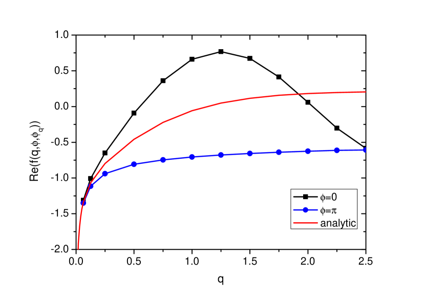
a)

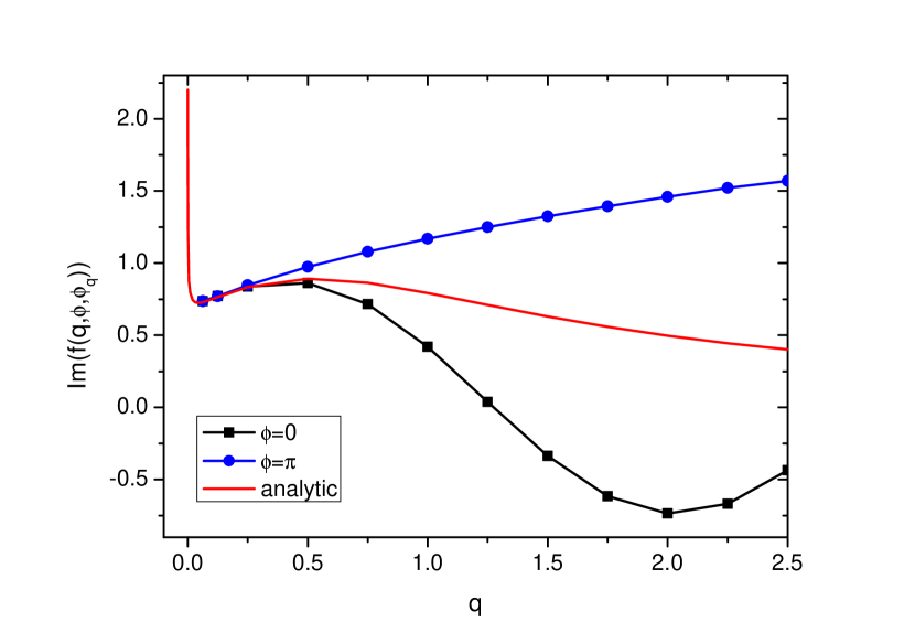
b)

Figure 1: (Color online) The dependence of real a) and imaginary b) part of the scattering amplitude on the momentum $q$ for the potential barrier (20) with circular base $a(\phi)=a_{0}=1$ and $U_{0}=10^{4}$. Calculations were carried out for $\phi_{q}=0$ with the parameters: $M=10^{2}$, $N=10^{5}$ and $\rho_{N}=15$. The quantities $f$ and $q$ are given in the units $\hbar=\mu=1$.

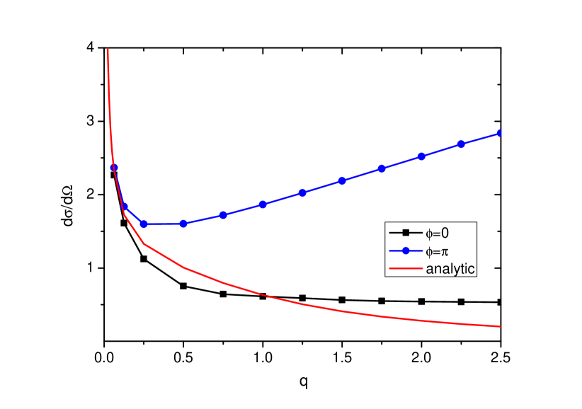
Figure 2: (Color online) The dependence of the differential cross section on the momentum $q$ for the potential barrier (20) with circular base $a(\phi)=a_{0}=1$ and $U_{0}=10^{4}$. Calculations were carried out for $\phi_{q}=0$ with the parameters: $M=10^{2}$, $N=10^{5}$ and $\rho_{N}=15$. The quantities $d\sigma/d\Omega$ and $q$ are given in the units $\hbar=\mu=1$.

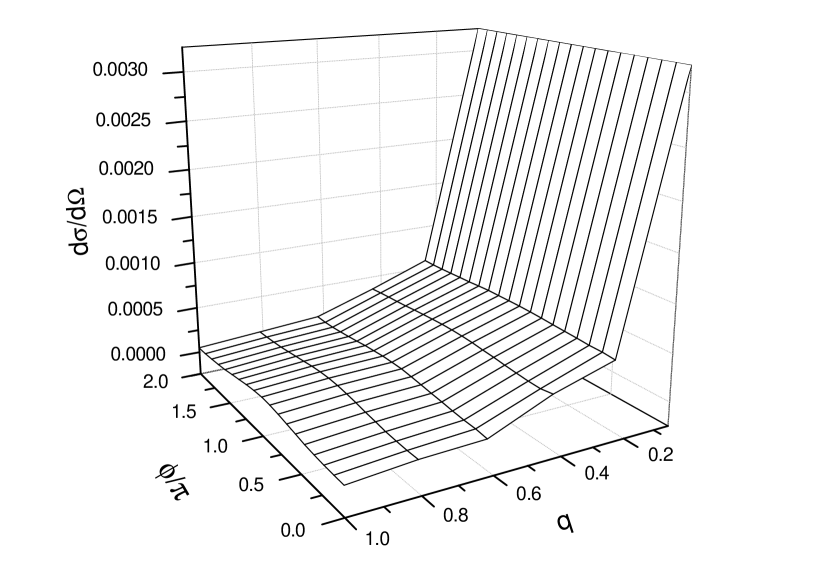
Figure 3: The dependence of the differential cross section on the momentum $q$ and scattering angle $\phi$ in the case of potential barrier (20) with $U_{0}=10^{3}$ and circular base $a(\phi)=a_{0}=1$. Calculations were carried out for $\phi_{q}=0$ with the parameters: $M=10^{2}$, $N=10^{5}$ and $\rho_{N}=15$. The quantities $d\sigma/d\Omega$ and $q$ are given in the units $\hbar=\mu=1$.

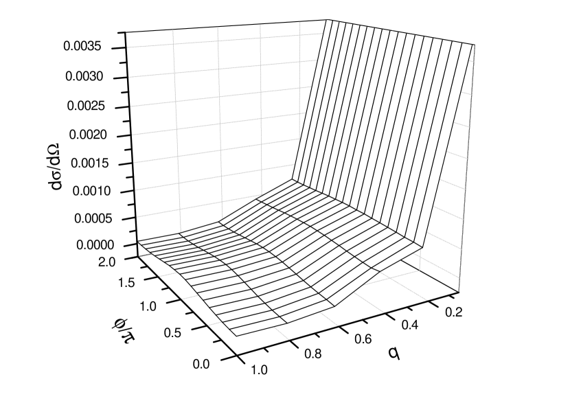
Figure 4: The dependence of the differential cross section on the momentum $q$ and scattering angle $\phi$ in the case of potential barrier (20) with $U_{0}=10^{3}$ and elliptic base with $a(\pi/2)=1.1$ and $a(0)=1$. Calculations were carried out for $\phi_{q}=0$ with the parameters: $M=10^{2}$, $N=10^{5}$ and $\rho_{N}=15$. The quantities $d\sigma/d\Omega$ and $q$ are given in the units $\hbar=\mu=1$.

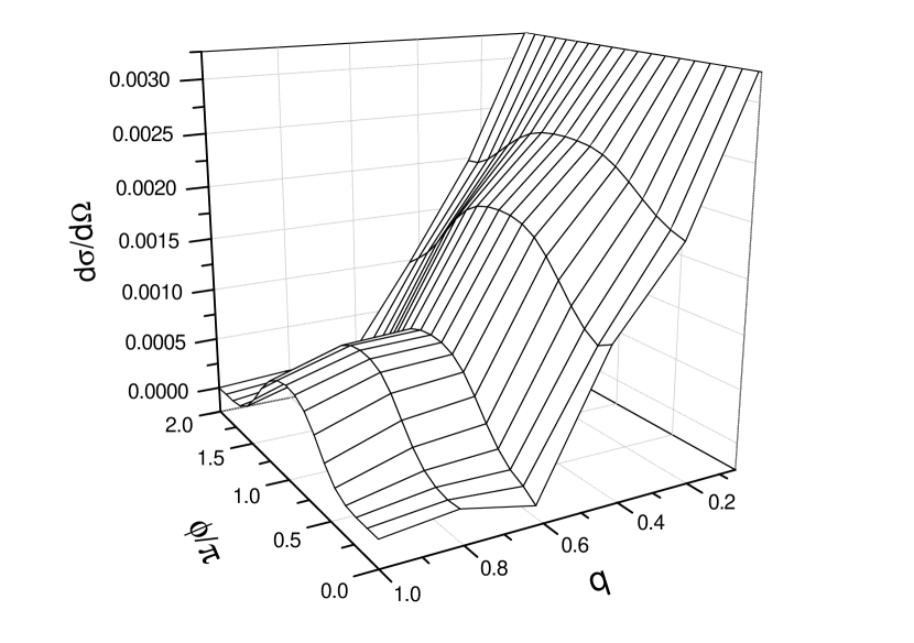
Figure 5: The same as in Fig. 4 but for the case of strong anisotropy of the scatterer (20) with $a(\pi/2)=2$ and $a(0)=1$. The quantities $d\sigma/d\Omega$ and $q$ are given in the units $\hbar=\mu=1$.

III.2 Dipole-dipole scattering in plane

Here we analyze the 2D quantum scattering on the long-range anisotropic scatterer defined by the dipole-dipole interaction. This problem simulates the collisions of polar molecules in pancake optical traps. The interaction potential between two arbitrarily oriented dipoles reads

$$U({\bm{\rho}},{\bm{d}}_{1},{\bm{d}}_{2})=\frac{1}{\rho^{3}}\left(({\bm{d}}_{1}{\bm{d}}_{2})-3\frac{({\bm{d}}_{1}{\bm{\rho}})({\bm{d}}_{2}{\bm{\rho}})}{\rho^{2}}\right)\,,$$ (22)

where ${\bm{d}}_{i},(i=1,2)$ – dipole moments and $({\bm{d}}_{i}{\bm{\rho}})/\rho$ – their projections onto the collision axis. The expression (22) can be written in the polar coordinates

$$U\left({\rho,\phi;\alpha,\beta,\gamma}\right)=\frac{d_{1}d_{2}}{\rho^{3}}[\sin(\alpha)\sin(\gamma)\cos(\beta)+$$

$$+\cos(\alpha)\cos(\gamma)-3\sin(\alpha)\sin(\gamma)\cos(\phi)\cos(\phi-\beta)]\,,$$ (23)

where the angles $\alpha$ and $\gamma$ define the tilt of dipoles to the scattering plane $XY$ and the angle $\beta$ denotes the mutual orientation of the dipole polarization planes $Zd_{1}$ and $Zd_{2}$ in Fig. 6.

If we consider the scenario when the polarization of colliding molecules is orthogonal to the plane of motion $\left({\alpha=\beta=\gamma=0}\right)$, interaction is fully isotropic and repulsive

$$U\left(\rho\right)=\frac{d_{1}d_{2}}{\rho^{3}}\,.$$ (24)

This case was intensively studied in the previous works ref16 ; ref18 .

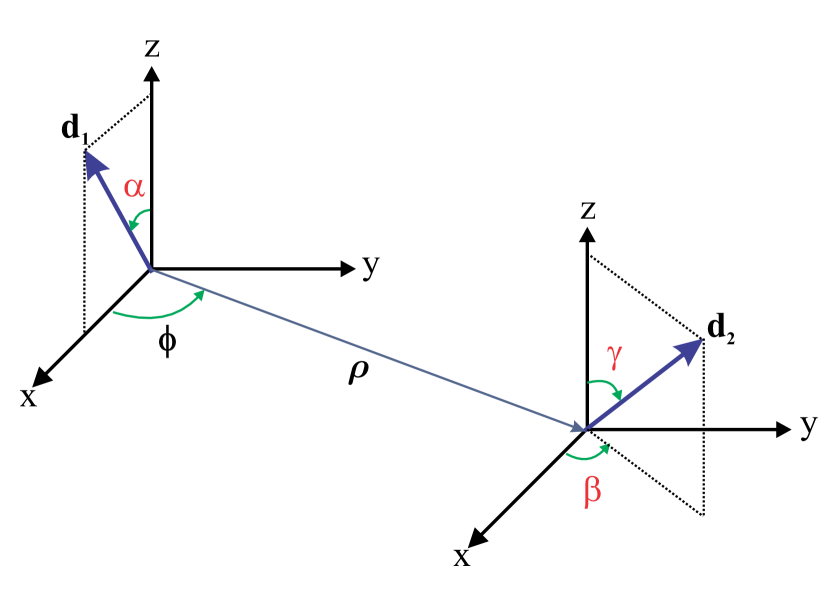
Figure 6: (Color online) Collision in the plane $XY$ of two arbitrarily oriented dipoles ${\bm{d}}_{1}$ and ${\bm{d}}_{2}$

For dipoles oriented in the plane $\left({\alpha=\gamma=\tfrac{\pi}{2}}\right)$, anisotropy arises and the interaction potential reads

$$U\left({\rho,\phi,\beta}\right)=\frac{d_{1}d_{2}}{\rho^{3}}[\cos(\beta)-3\cos(\phi)\cos(\phi-\beta)]\,.$$ (25)

A particular case of parallel dipoles with the polarization axis tilted to the plane of motion ($\alpha=\gamma;\mbox{ }\beta=0)$ with short-range interaction modeled by a hard wall at the origin

$$V_{HW}(\rho)=\left\{{{\begin{array}[]{*{20}c}{\infty,\mbox{ }\rho\leqslant\rho_{HW}\hfill}\\ {0,\mbox{ }\rho>\rho_{HW}\hfill}\\ \end{array}}}\right.$$ (26)

with the width ${\rho_{HW}}\mathord{\left/{\vphantom{{\rho_{HW}}D}}\right.\kern-1.2pt}D=0.1$

$$U\left({\rho,\phi,\alpha}\right)=V_{HW}(\rho)+\frac{d^{2}}{\rho^{3}}[1-3\sin^{2}(\alpha)\cos^{2}(\phi)]$$ (27)

was considered in paper ref17 . We have investigated this case with our approach and have obtained good agreement with the results of paper ref17 . This is illustrated by Fig. 7, where the calculated total cross section $\sigma(q,\alpha)$ (5) is given in the units of $\sigma_{SC}$. Here $D$ is the dipolar length $D={\mu d^{2}}\mathord{\left/{\vphantom{{\mu d^{2}}{\hbar^{2}}}}\right.\kern-1.2pt}{\hbar^{2}}\mbox{ (}d=d_{1}=d_{2})$ and $\sigma_{SC}=\tfrac{4}{q}\sqrt{\pi Dq}$ is the value of the total scattering cross section in the eikonal approximation that is valid in the high-energy regime, $Dq\gg 1$ ref17 . All calculations in this section were performed for the following parameters: $M=40\,,\,N=1.2\times 10^{5}$ and $\rho_{N}=60$; the number of grid points on $\phi_{q}$ was $2M_{q}+1=101$.

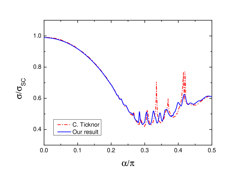
Figure 7: (Color online) A comparison of the total cross section (in the units of $\sigma_{SC}$) with the result of C. Ticknor ref17 calculated for potential (27) at $D=1\,\,,\,Dq=10$.

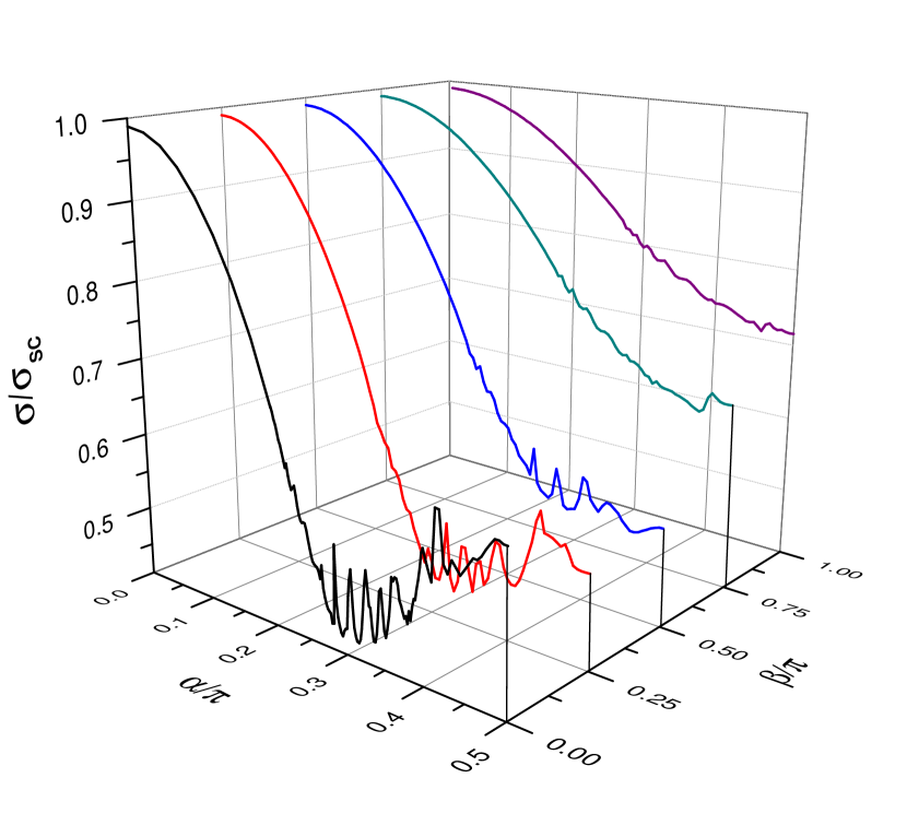
Figure 8: (Color online) The total cross sections $\sigma$ in the units of $\sigma_{SC}$ as a function of the dipole tilt angle $\alpha=\gamma$ and the rotational angle $\beta$ calculated for potential (III.2) at $D=1\,\,,\,Dq=10$.

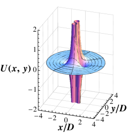
$\beta=0,\mbox{ }\alpha=0.25\pi$

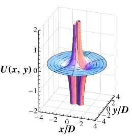
$\beta=0,\mbox{ }\alpha=0.35\pi$

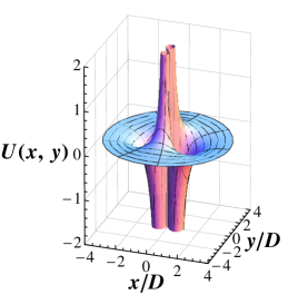
$\beta=0,\mbox{ }\alpha=0.5\pi$

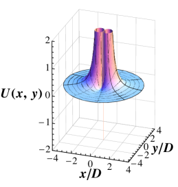
$\beta=\pi,\mbox{ }\alpha=0.25\pi$

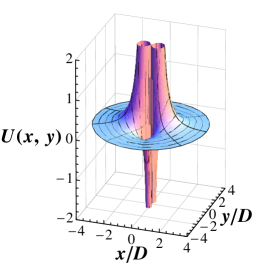
$\beta=\pi,\mbox{ }\alpha=0.35\pi$

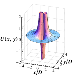
$\beta=\pi,\mbox{ }\alpha=0.5\pi$

Figure 9: (Color online) The dependence of the dipole-dipole potential $U({\bm{\rho}},{\bm{d}_{1}},{\bm{d}_{2}})$ (III.2) in the units of $E_{D}=\hbar^{6}/\mu^{3}d^{4}$ ($d=d_{1}=d_{2}$) on the tilt angle $\alpha$ for two extreme mutual orientations $\beta=0$ and $\pi$ of the dipole polarization planes $Zd_{1}$ and $Zd_{2}$.

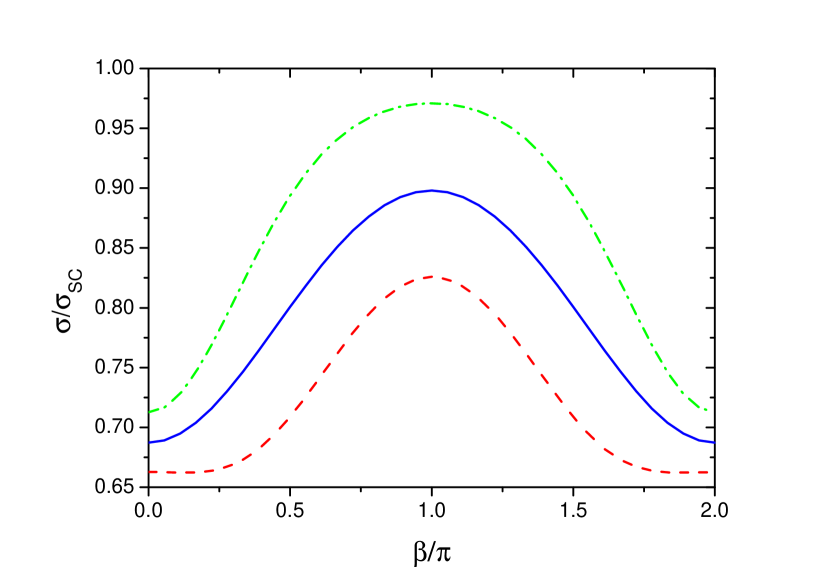
Figure 10: (Color online) The total cross section $\sigma$ (solid line), bosonic cross section $\sigma_{g}$ (dashed line) and fermionic cross section $\sigma_{u}$ (dash-dot line) calculated for potential (III.2) as a function of the angle $\beta$ for the fixed $\alpha=0.2\pi$ at $D=1\,\,,\,Dq=10$ (in the units of $\sigma_{SC}$).

Then, we have analyzed how the found “resonant” structure for the polarized dipoles (see Fig. 7) in the calculated dependence of the scattering cross section on the dipole tilt angle $\alpha=\gamma$ varies with destroying the polarization. Depolarization was simulated by rotating the angle $\beta$ between the dipole polarization planes $Zd_{1}$ and $Zd_{2}$ (see Fig. 6). We found progressive narrowing of the “resonance” area with a simultaneous decrease of the amplitudes of the “resonance” oscillations with increasing angle $\beta$ from $0$ to $\pi$ (see Fig. 8). When approaching the point $\pi$ the “resonant” structure disappears, the cross section becomes smooth relative to $\alpha$ and reaches its maximum value. This effect is due to the fact that when approaching the angle $\beta=\pi$ repulsive feature of the dipole-dipole interaction becomes dominant (see Fig. 9). With decreasing $\beta$ from $\pi$ to $0$ the attractive part $U(\rho,\phi)<0$ appears for some $\rho$ and $\phi$. It leads to appearing the “resonant” part in the scattering cross section. Note, that the presented cross sections were obtained for distinguishable particles. The effect of symmetrization/antisymmetrization $f_{g,u}(\phi)=(f(\phi)\pm f(\phi-\pi))/\sqrt{2}$ (i.e. transition to identical particles) is shown in Fig. 10 for $\alpha=0.2\pi$ and $\beta$ varying from $0$ to $2\pi$, where we observe the strong dependence of the total cross sections on the angle $\beta$ with the maximal enhancement at $\beta=\pi$. The cross sections are symmetric with respect to this point. We have to note that the curves $\sigma_{g}(\beta)$ and $\sigma_{u}(\beta)$ describing the scattering of bosonic and fermionic particles exactly repeat the behavior of the curve $\sigma(\beta)$ for distinguishable particles.

Finally, we have analyzed the scattering of arbitrarily oriented dipoles in the case of mutual orthogonality of their polarization planes $Zd_{1}$ and $Zd_{2}$ ($\beta=\pi/2$). Here also we found a strong “resonant” structure by the tilt angle $\gamma$ of one dipole, if the other dipole is oriented in the scattering plane $XY$ ($\alpha=\beta=\pi/2$) (see Fig. 11), that appears due to the attractive feature of the dipole-dipole interaction strength with increasing of the tilt angle $\alpha\rightarrow\pi/2$.

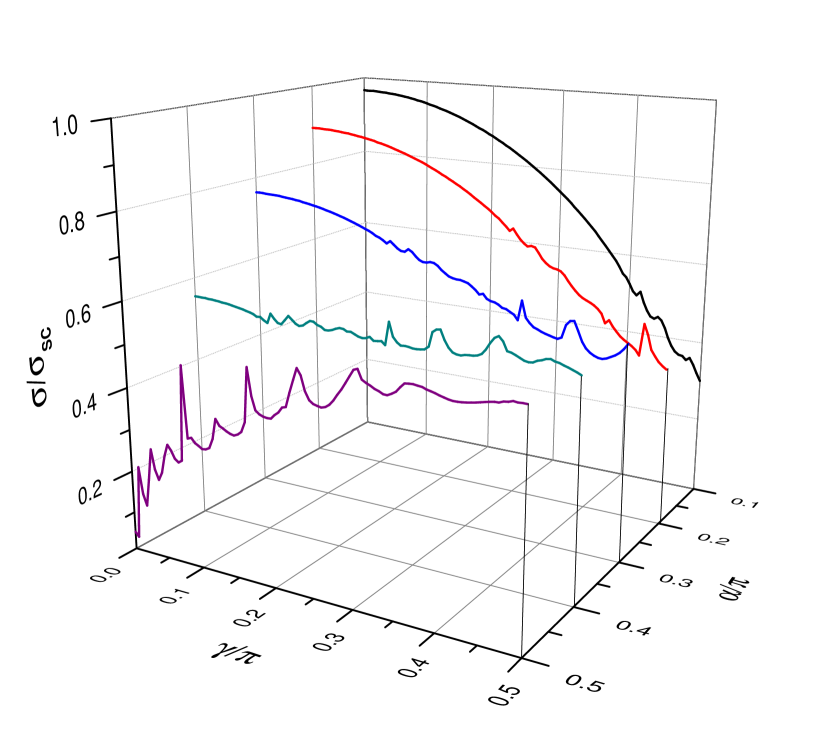
Figure 11: (Color online) The total cross sections $\sigma$ in the units of $\sigma_{SC}$ as a function of the dipole tilt angles $\alpha$ and $\gamma$ calculated for potential (III.2) at $D=1\,\,,\,Dq=10$. The rotational angle $\beta$ is equal to $\pi/2$.

III.3 Advantages and prospects of the angular-grid representation

Let us discuss here the advantages of our angular-grid representation (7) in comparison with the traditional partial-wave formalism, which was used in particular by Ticknor in the analysis of the 2D scattering of polarized dipoles ref17 .

First, for any potential $U(\rho,\phi)$ the estimate of the residual term $\delta\Psi_{M}$ in the expansion $\Psi(\rho,\phi)=\sum_{m=-M}^{M}\chi_{m}(\rho)e^{im\phi}/\sqrt{\rho}+\delta\Psi_{M}$ of the desired wave function on partial waves is unknown. This fact becomes crucial in the case of strongly anisotropic and long-range potential considered in the above Subsection III.B, where the partial-wave expansion becomes very slow due to the strong coupling between different angular momenta remaining even at the zero-energy limit ref14 ; ref15 . Opposite, our angular-grid representation belongs to a class of mesh methods admitting an estimate of an approximation error. Thus, since the representation (7) can be considered, following ref21 , as a Fourier interpolation of the order $M$ in the variable $\phi$, the error of the approximation (7) can be estimated as ref29

$$\delta\Psi_{M}=|\Psi(\rho,\phi)-\sum_{j=0}^{2M}\omega_{j}(\phi)\Psi(\rho,\phi_{j})|<const\frac{\ln M}{M^{k}}\,,$$

where $\omega_{j}(\phi)=\frac{2\pi}{(2M+1)}\sum_{m=-M}^{M}e^{im(\phi-\phi_{j})}$ and $k$ is the number of existing continuous and bounded derivatives over $\phi$. Due to this estimate one can await a rapid convergence of our angular-grid representation (7) with increasing $M$ on the sequence of compressed grids $\{\phi_{j}\}_{0}^{2M}$. It was confirmed in all the computations we performed (see also illustration of the convergence of the angular-grid representation given in Table.II of Appendix B). The convergent results were obtained even in the regions of “resonant” scattering of polarized as well as unpolarized dipoles (see Figs.7,8 and 11). Slight shifts of the positions of the “resonances” in the scattering of polarized dipoles calculated with our method relative to the values obtained by Ticknor (see Fig.7) can be explained by the error due to the truncation of his partial-wave sum.

Another important advantage of the angular-grid representation is its flexibility connected with the lack of the time-consuming procedure of calculating the matrix elements of the interaction potential. As was mentioned above, the potential matrix in this representation is diagonal and consists of the values of the potential in the angular grid nodes. This circumstance permitted us to perform extended detail computations of the 2D dipole-dipole scattering of the different mutual orientations. This also makes the method very perspective in the case of nonseparable interactions and generalization to higher dimensions.

IV Conclusion

We have developed a computational scheme for quantitative analysis of the 2D quantum scattering on the long-range anisotropic potentials. High efficiency of the method was demonstrated in the analysis of scattering on the cylindrical potential with the elliptical base and dipole-dipole collisions in the plane. In the last case we found the strong dependence of the scattering cross section on the mutual orientation of dipoles.

The method can be applicable for analyzing the collisional dynamics of the polarized as well as unpolarized polar molecules in 2D and quasi-2D traps. A natural application is the quantitative analysis of the confinement-induced resonances (CIR) in quasi-2D traps. In this problem the crucial element is an inclusion of the transverse confinement what we suppose to explore in our future work with generalization of the developed approach to this 3D case. Particularly, this analysis can resolve the puzzle with the position of the 2D CIR measured recently ref27 , which is under intensive discussions.

Table 2: The dependence of the scattering amplitude $f(q,\phi,\phi_{q})$ on the number of angular-grid points for the scatterer (20) with elliptical base. Calculations were performed for $q=1.5$ with the parameters: $U_{0}=10^{3},\quad N=10^{4}$, and $\rho_{N}=15$.

	$\mbox{ }a(\pi/2)/a(0)=1.1$		$\mbox{ }a(\pi/2)/a(0)=2.0$
$M$	$f(q,0,0)$	$f(q,\pi,0)$	$f(q,0,0)$	$f(q,\pi,0)$
1	0.94212 - i0.36446	-0.33027 + i1.24225	-0.95099 - i0.52976	0.36649 + i1.04884
2	0.65275 – i0.30331	-0.61946 + i1.30336	-1.48979 + i0.79336	-0.50755 + i2.02677
3	0.68693 – i0.30254	-0.65392 + i1.30275	-0.31229 + i0.79336	-1.01013 + i1.68129
4	0.68794 – i0.30507	-0.65902 + i1.29149	-0.28629 + i0.18596	-0.90989 + i1.50458
5	0.68799 – i0.30506	-0.65940 + i1.29164	-0.50155 + i0.05523	-0.87486 + i1.52425
10			-0.60611 + i0.07641	-0.89428 + i1.53586
20			-0.61098 + i0.07836	-0.89552 + i1.53816
30			-0.61173 + i0.07971	-0.89572 + i1.53885

Appendix A Finite-difference approximation for boundary-value problem (10),(11) and (15)

The boundary-value problem (II),(11) and (II), obtained in Section II in the angular-grid representation (7), reads in a matrix form as:

$$\left\{{\begin{array}[]{l}\rho^{2}\frac{d^{2}}{d\rho^{2}}\bm{\psi}(\rho)+\left[{\frac{1}{4}\hat{I}+\frac{2\mu}{\hbar^{2}}\rho^{2}\left({E\hat{I}-\hat{U}(\rho)}\right)}\right]\bm{\psi}(\rho)\,+\\ \hskip 142.26378pt+\,\hat{h}^{(0)}\bm{\psi}(\rho)=0\\ \bm{\psi}\xrightarrow[\rho\to 0]{}const\cdot\sqrt{\rho}\\ \frac{2\pi}{(2M+1)\sqrt{\rho}}\sum\limits_{j=0}^{2M}{e^{-im\phi_{j}}\psi_{j}(\rho)}=i^{m}J_{m}(q\rho)\sqrt{2\pi}+\\ \hskip 142.26378pt+\,\frac{f_{m}(\phi_{q})}{\sqrt{-i\rho}}e^{iq\rho}\,,\\ \end{array}}\right.$$ (28)

where $h^{(0)}_{jj^{\prime}}=-\frac{2\pi}{(2M+1)}\sum\limits_{m=-M}^{M}{m^{2}e^{im(\phi_{j}-\phi_{j^{\prime}})}\,,\,\hat{U}(\rho)=}$ $\mathrm{diag}\left({U(\rho,\phi_{q},\phi_{0}),U(\rho,\phi_{q},\phi_{1}),\ldots,U(\rho,\phi_{q},\phi_{2M})}\right)$ and $\bm{\psi}(\rho)=\{\psi(\rho,\phi_{0}),\psi(\rho,\phi_{1}),\ldots\psi(\rho,\phi_{2M})\}$. In this representation the angular dependence is built into the matrix $\hat{h}^{(0)}$ and the interaction is included into the diagonal matrix $\hat{U}(\rho)$ of values of the potential in the angular grid nodes. The constant matrix $\hat{h}^{(0)}$ couples all equations in a system and does not depend on the radial variable. There is no need to compute any matrix elements of the potential, what essentially minimizes the computational costs.

For solving boundary value problem (28) the seven-point finite-difference approximation for second derivatives of sixth order

$$\frac{d^{2}}{d\rho^{2}}\bm{\psi}_{n}=\frac{1}{180h^{2}}\left(2\bm{\psi}_{n-3}-27\bm{\psi}_{n-2}+270\bm{\psi}_{n-1}\right.$$

$$\left.-490\bm{\psi}_{n}+270\bm{\psi}_{n+1}-27\bm{\psi}_{n+2}+2\bm{\psi}^{n+3}\right)+O(h^{6})$$ (29)

is applied in the points $\rho_{n}$ of the radial grid, where $\bm{\psi}_{n}\equiv\bm{\psi}(\rho_{n}),\mbox{ (}n=3,4,\ldots,N-3\mbox{)}$. As a result, the system (28) reduces to the system of linear algebraic equations (II) with the matrix $\hat{A}$ whose band structure reads

$$\sum_{n^{\prime}=n-3}^{n+3}\hat{A}_{nn^{\prime}}\bm{\psi}_{n}=\bm{F}_{n}\,\,,$$ (30)

where the $\hat{A}_{nn^{\prime}}$ coefficients are the square $(2M+1)\times(2M+1)$ matrices, and the elements $\bm{F}_{n}$ of the right-side of (30) are the $2M+1$ dimensional vectors. After employing the “right-side” boundary condition in the form (II) in the last three grid points $n=N-2,N-1,N$ and, analogously, the “left-side” boundary condition in the form (II) in the first two points $n=1,2$, the detailed structure of the matrix $\hat{A}$ is represented as

$$\left\{{\begin{array}[]{l}\sum_{n^{\prime}=n}^{n+1}\hat{A}_{nn^{\prime}}\bm{\psi}_{n^{\prime}}=\bm{F}_{n}\,\,,\,\,\,\,\,\,n=1,2\\ \sum_{n^{\prime}=n-3}^{n+3}\hat{A}_{nn^{\prime}}\bm{\psi}_{n^{\prime}}=0\,\,,\,\,\,\,\,n=3,4,..,N-3\\ \sum_{n^{\prime}=n-1}^{n}\hat{A}_{nn^{\prime}}\bm{\psi}_{n^{\prime}}=\bm{F}_{n}\,\,,\,\,n=N-2,N-1,N\,.\\ \end{array}}\right.$$ (31)

The block structure of the system (31) provides several significant advantages. The block matrix can be stored in a packaged form, which allows the use of optimal resource. The system (31) can be efficiently solved by a fast implicit matrix algorithm based on the idea of the block sweep method ref25 .

Appendix B Convergence of computational scheme

In the Table 2 we illustrate the convergence of the calculated scattering amplitude $f(q,\phi,\phi_{q})$ over the number of angular grid points $2M+1$ for the scatterers with weak and essential anisotropy at ${a(\pi\mathord{\left/{\vphantom{\pi 2}}\right.\kern-1.2pt}2)}\mathord{\left/{\vphantom{{a(\pi\mathord{\left/{\vphantom{\pi 2}}\right.\kern-1.2pt}2)}{a(0)}}}\right.\kern-1.2pt}{a(0)}=1.1\mbox{ and }2$ in the potential barrier (20). For the case ${a(\pi\mathord{\left/{\vphantom{\pi 2}}\right.\kern-1.2pt}2)}\mathord{\left/{\vphantom{{a(\pi\mathord{\left/{\vphantom{\pi 2}}\right.\kern-1.2pt}2)}{a(0)}}}\right.\kern-1.2pt}{a(0)}=1.1$ we reach the accuracy of four significant digits in the scattering amplitude on the angular grids with $M=5$. For stronger anisotropy ${a(\pi\mathord{\left/{\vphantom{\pi 2}}\right.\kern-1.2pt}2)}\mathord{\left/{\vphantom{{a(\pi\mathord{\left/{\vphantom{\pi 2}}\right.\kern-1.2pt}2)}{a(0)}}}\right.\kern-1.2pt}{a(0)}=2$ the accuracy of two significant digits was reached at $M=30$.

The number of radial grids $N$ and the border of integration $\rho_{N}$ were chosen to keep the accuracy of four significant digits in the calculated amplitudes.

References

- (1) M. A. Baranov, Phys. Rep. 464, 71 (2008).
- (2) I. Bloch, J. Dalibard and W. Zwerger, Rev. Mod. Phys. 80, 885 (2008).
- (3) C. Ticknor, R. M. Wilson and J. L. Bohn, Phys. Rev. Lett. 106, 065301 (2011).
- (4) G. M. Brunn and E. Taylor, Phys. Rev. Lett. 101, 245301 (2008).
- (5) J. C. Cremon, G. M. Brunn and S. M. Reimann, Phys. Rev. Lett. 105, 255301 (2010).
- (6) K.-K. Ni et. al., Science 322, 231 (2008); S.Ospelkaus et. al., Science 327, 853 (2010).
- (7) L. D. Carr et. al., New J. Phys 11, 055049 (2009).
- (8) M. H. G. de Miranda et. al., Nat. Phys. 7, 502 (2011).
- (9) P. Minnhagen, Rev. Mod. Phys. 59, 1001 (1987).
- (10) P. A. Lee, N. Nagaosa and X.-G. Wen, Rev. Mod. Phys. 78, 17 (2006).
- (11) K. S. Novoselov, Rev. Mod. Phys. 83, 837 (2011).
- (12) C. Nayak, S. H. Simon, A. Stern, M. Freedman and S. D. Sarma, Rev. Mod. Phys. 80, 1083 (2008).
- (13) K. Martiyanov, V. Makhalov and A. Turlapov, Phys. Rev. Lett. 105, 030404 (2010); A. Turlapov, JETP Letters 95, 96 (2012).
- (14) M. Marinescu and L. You, Phys. Rev. Lett. 81, 4596 (1998); B. Deb and L. You. Phys. Rev. A 64, 022717 (2001)
- (15) V. S. Melezhik and Chi-Yu Hu, Phys. Rev. Lett. 90, 083201 (2003).
- (16) C. Ticknor, Phys. Rev. A 80, 052702 (2009).
- (17) C. Ticknor, Phys. Rev. A 84, 032702 (2011).
- (18) C. Ticknor, Phys. Rev. A 81, 042708 (2010).
- (19) J. P. D’Incao and C. H. Greene, Phys. Rev. A 83, 030702 (2011).
- (20) Z. Li, S. V. Alyabishev and R. V. Krems, Phys. Rev. Lett. 100, 073202 (2008).
- (21) V. S. Melezhik, J. Comput. Phys. 92, 67-81 (1991).
- (22) L. D. Landau and E. M. Lifshitz, in Quantum mechanics: Non-Relativistic Theory, Vol. 3 (Pergamon Press, 1977) 3rd ed., Chap. 132, pp. 551–552.
- (23) D. S. Petrov and G. V. Shlyapnikov, Phys. Rev. A 64, 012706 (2001).
- (24) L. D. Landau and E. M. Lifshitz, in Quantum mechanics: Non-Relativistic Theory, Vol. 3 (Pergamon Press, 1977) 3rd ed., Chap. 123, pp. 507–508.
- (25) M. Abramowitz and A. I. Stegun, Handbook of Mathematical Functions (U.S. National Bureau of Standards, 1965).
- (26) I. M. Gelfand and S. V. Fomin, Calculus of Variations (Dover Publications, New York, 2000).
- (27) W. H. Press, S. A. Teukolsky, W. T. Vetterling, and B. P. Flannery, Numerical Recipes (Cambridge University Press, Cambridge, 1992).
- (28) V. V. Pupyshev, Phys. Atom. Nucl. 77, 664 (2014).
- (29) A. N. Kolmogorov, Ann. Math. 35, 521 (1935).
- (30) E. Haller et. al., Phys. Rev. Lett. 104, 153203 (2010).