The fundamental solution of the unidirectional pulse propagation equation

Abstract

The fundamental solution of a variant of the three-dimensional wave equation known as “unidirectional pulse propagation equation” (UPPE) and its paraxial approximation is obtained. It is shown that the fundamental solution can be presented as a projection of a fundamental solution of the wave equation to some functional subspace. We discuss the degree of equivalence of the UPPE and the wave equation in this respect. In particular, we show that the UPPE, in contrast to the common belief, describes wave propagation in both longitudinal and temporal directions, and, thereby, its fundamental solution possesses a non-causal character.

I Introduction

Often in physics, the problem of light propagation in a nonlinear, homogeneous isotropic medium requires solving the nonlinear wave equation (WE)

$$\square E(\mathrm{\mathbf{r}},t)\equiv\Delta E(\mathrm{\mathbf{r}},t)-\frac{1}{c^{2}}\partial_{tt}E(\mathrm{\mathbf{r}},t)=Q[E],$$ (1)

where $\mathrm{\mathbf{r}}=\{x,y,z\}$ is a point of $\mathbb{R}^{3}$ locating the spatial coordinates, $t$ is time, $\Delta=\partial_{zz}+\partial_{yy}+\partial_{xx}$, and $E(\mathrm{\mathbf{r}},t)\in\mathbb{R}$ represents the electric field. In the following, we apply the scalar field assumption and suppose that the linear polarization and nonlinearity possibly entering $Q[E]$ do not alter the polarization state. $Q[E]$ is, in general, a nonlinear operator describing the medium response. For instance, for the case of an electromagnetic wave propagating in a plasma, we have $Q=\mu_{0}\partial_{t}J$, where $J$ is the plasma current density and $\mu_{0}$ is the vacuum permeability. In the case of strong optical fields, the quantity $J$ depends itself on $E$ in rather complicated way Marr (1967); Bergé et al. (2007); Couairon and Mysyrowicz (2007); Brabec (2008), making the equation nonlinear.

Independently on the nature of inhomogeneity $Q$, the solving for Eq. (1) needs both initial and boundary conditions. Unfortunately, this problem is, in large number of practically important cases, difficult to treat numerically. A typical situation is a propagation of a few-cycle pulse through a waveguide Husakou and Herrmann (2001); Fedotova, Husakou, and Herrmann (2006); Babushkin et al. (2007); Babushkin, Noack, and Herrmann (2008); Babushkin, Skupin, and Herrmann (2010); Leblond and Mihalache (2013); Demircan, Amiranashvili, and Steinmeyer (2011); Köhler et al. (2011); Babushkin et al. (2011); Demircan et al. (2012); Bergé et al. (2013) or in a long filament Bergé et al. (2013, 2007), which assumes large extent in one spatial dimension (say, $z$), making the amount of data required for solving the initial value problem extremely large. To deal with such cases, Unidirectional Pulse Propagation Equations (UPPE) have been proposed Kolesik and Moloney (2004); Bergé et al. (2007). One of the most well-known models aims at describing the so-called ”forward” (propagating along positive longitudinal coordinates, $z>0$) component of the pulse electric field in Fourier domain along the $\{x,y,t\}$ variables. It governs the Fourier-transformed electric field $\tilde{E}(z,\mathrm{\mathbf{k}}_{\bot},\omega)\in\mathbb{C}$ as

$$\partial_{z}\tilde{E}(z,\mathrm{\mathbf{k}}_{\bot},\omega)-i\beta_{z}\tilde{E}(z,\mathrm{\mathbf{k}}_{\bot},\omega)=\frac{1}{2i\beta_{z}}\tilde{Q}(z,\mathrm{\mathbf{k}}_{\bot},\omega).$$ (2)

Here, $\tilde{E}(z,k_{x},k_{y},\omega)=\mathcal{F}_{x,y,t}\left[E(x,y,z,t)\right]$, $\tilde{Q}=\mathcal{F}_{x,y,t}\left[Q\right]$, $\mathcal{F}_{x,y,t}\left[\cdot\right]$ is the Fourier transform from variables $\{x,y,t\}$ to $\{k_{x},k_{y},\omega\}$, namely, when using $\mathrm{\mathbf{r}}_{\bot}=\{x,y\}$ and $\mathrm{\mathbf{k}}_{\bot}=\{k_{x},k_{y}\}$:

$$\mathcal{F}_{{\mathrm{\mathbf{r}}}_{\bot},t}\left[f\right]{(z,{\mathrm{\mathbf{k}}}_{\bot},\omega)=\int f({\mathrm{\mathbf{r}}},t)\exp{(-i{\mathrm{\mathbf{k}}}_{\bot}{\mathrm{\mathbf{r}}}_{\bot}+i\omega t)}}dxdydt,$$ (3)

for a given integrable function $f$, while $\beta_{z}=\sqrt{\omega^{2}/c^{2}-k_{\bot}^{2}}$.

Equation (2) can be easily rewritten using the original variables $\{\mathrm{\mathbf{r}},t\}$:

$$\partial_{z}E(\mathrm{\mathbf{r}},t)-i\Phi\star E(\mathrm{\mathbf{r}},t)=\frac{1}{2i}\Psi\star Q(\mathrm{\mathbf{r}},t),$$ (4)

where

$$\Phi=\mathcal{F}_{k_{x},k_{y},\omega}^{-1}\left[\beta_{z}\right];\,\,\,\Psi=\mathcal{F}_{k_{x},k_{y},\omega}^{-1}\left[1/\beta_{z}\right],$$ (5)

and $\star$ stands for the convolution operator with respect to the variables $\{x,y,t\}$.

In contrast to Eq. (1), Eq. (4) is not PDE anymore, but it belongs to the class of pseudo-differential equations. Unlike Eq. (1) which is commonly integrated in time under specific conditions on boundaries and field derivatives, Eq. (4) only requests the field value $E(x,y,t)$ at $z=0$ and boundary conditions in the transverse $(x,y)$ dimensions; it is then solved along the longitudinal direction $z>0$. Equation (2) results from a kind of factorization of the original wave equation (1), typically Kolesik and Moloney (2004); Bergé et al. (2007); Kinsler (2010) (but not necessarily Amiranashvili and Demircan (2010)) neglecting the waves propagating backward in $z$-direction. Shortly, factorization can easily be made by proceeding as follows. After applying the Fourier transform $\mathcal{F}_{\{x,y,t\}}$, Eq. (1) can be written as

$$(\partial_{z}-i\beta_{z})(\partial_{z}+i\beta_{z})\tilde{E}=\tilde{Q}.$$ (6)

Now, we decompose the field $\tilde{E}$ into the sum $\tilde{E}=\tilde{E}_{-}e^{-i\beta_{z}z}+\tilde{E}_{+}e^{+i\beta_{z}z}$, assuming that $\tilde{E}_{\pm}$ varies in $z$ much slower than the exponential term, that is, $(\partial_{z}+i\beta_{z})\tilde{E}_{+}e^{+i\beta_{z}z}\approx 2i\beta_{z}\tilde{E}_{+}e^{+i\beta_{z}z}$. The same decomposition into $\tilde{Q}_{+}$, $\tilde{Q}_{-}$ is made for $\tilde{Q}$. Substituting the previous quantities into Eq. (6), multiplying it by $e^{+i\beta_{z}z}$ and integrating over some short range $z$ we obtain $2i\beta_{z}(\partial_{z}-i\beta_{z})\tilde{E}_{+}=\tilde{Q}_{+}$. Now, if we assume that both the field $\tilde{E}$ and the inhomogeneity $\tilde{Q}$ contain only the part corresponding to $\tilde{E}_{+}$ ($\tilde{Q}_{+}$), we then arrive to Eq. (2). In this simple derivation, it is explicitly assumed that the amplitude $E_{+}$ is slow compared to $e^{+i\beta_{z}z}$. This assumption is not necessary if more involved projection techniques are used, which include decomposition of $E$ and $Q$ into some transverse modes Kolesik and Moloney (2004). These derive from the linear modes of Eq. (1), assuming weak nonlinearities.

Equation (2), its 1-dimensional analogs and other modifications are nowadays routinely utilized in optics to describe ultrashort pulses with ultrabroad spectra (see Husakou and Herrmann (2001); Fedotova, Husakou, and Herrmann (2006); Bergé et al. (2007); Babushkin and Herrmann (2008); Babushkin, Noack, and Herrmann (2008); Husakou and Herrmann (2009a, b); Im, Husakou, and Herrmann (2010); Amiranashvili and Demircan (2010); Babushkin, Skupin, and Herrmann (2010); Babushkin et al. (2010); Kolesik et al. (2010); Babushkin et al. (2011); Köhler et al. (2011); Demircan, Amiranashvili, and Steinmeyer (2011); Whalen et al. (2012); Andreasen and Kolesik (2012); Demircan et al. (2012); Leblond and Mihalache (2013); Bergé et al. (2013) and references therein), because they include minimal assumptions about the spectral width of $E(\mathrm{\mathbf{r}},t)$. A currently-met approximation is the paraxial assumption, $k_{z}\simeq k$, performed in the denominator of the $Q$ term in Eq. (2) Bergé et al. (2007), which signifies that the inhomogeneity is approached by the value defined by its forward component near the propagation axis. This approximation will be addressed at the end of the present work. Both Eq. (1) and Eq. (2) can be solved analytically only in exceptional cases. Nevertheless, if we consider the wave equation Eq. (1), a lot can be said about the general behavior of its solutions, considering the right hand side $Q$ as a pre-known quantity and thus Eq. (1) as a linear inhomogeneous PDE. In particular, in the plasma case with $Q=\mu_{0}J$, it is sometimes useful to consider an approximation in which the current $J$ does not depend on $E$ Nodland and McKinstrie (1997). Moreover, linear dispersion should in principle be treated when describing ultrashort pulses. Chromatic dispersion is embedded in the linear modes of Eq. (1), when one considers a frequency-dependent dielectric constant $\epsilon(\omega)$, and it usually intervenes through $\tilde{Q}=-(\omega^{2}/c^{2})\chi^{(1)}(\omega)\tilde{E}$, where $\chi^{(1)}$ denotes the first-order susceptibility tensor of the material. Accounting for noticeable variations of this quantity would, however, limit our analytic treatment. Therefore, for technical convenience, we shall consider the basic configuration in which the dielectric constant is constant.

Under these conditions, it is well-known that a solution of the linear inhomogeneous variant of Eq. (1) with a given, regular inhomogeneity $Q(\mathrm{\mathbf{r}},t)$ can be obtained using a fundamental solution approach with the help of tempered distributions, i.e., the solution (in the sense of generalized functions) is deduced from that with an inhomogeneity being a Dirac $\delta$-function, $Q=\delta(\mathrm{\mathbf{r}},t)$. The two most useful linearly-independent fundamental solutions of the D’Alembertian operator $\square$ are

$$\mathcal{E}_{\square\pm}=\frac{-1}{4\pi r}\delta(t\mp r/c),$$ (7)

where $r=|\mathrm{\mathbf{r}}|$. They describe spherical waves propagating forward ($\mathcal{E}_{\square+}$) or backward ($\mathcal{E}_{\square-}$) in time. From these two solutions, only $\mathcal{E}_{\square+}$ is physically meaningful, since it describes a response to an excitation (delta-function), that propagates in positive direction along time $t$ and thus respects the causality principle. By contrast, $\mathcal{E}_{\square-}\propto\delta(t+r/c)$ describes a response going ”backward” in time and thus being unphysical. Therefore, any solution of Eq. (1) for regular enough function $Q$ will physically make sense through the convolution product $\mathcal{E}_{\square+}\star Q$, whereas $\mathcal{E}_{\square-}\star Q$ cannot fulfill the causality principle.

Similarly, one can search for the fundamental solution of Eq. (4), that is, its generalized solution using the inhomogeneity $Q=\delta(\mathrm{\mathbf{r}},t)$. To the best of our knowledge, neither such a fundamental solution, nor its basic properties have been investigated so far to appreciate the applicability of the proposed UPPE models. Therefore, in the present article, we construct a fundamental solution of Eq. (4). We show that this solution is a projection of the fundamental solution of Eq. (1) to some functional subspace, formed by waves propagating either “forward-” or “backward-” in $z$-direction (see Theorem IV.1). We explore consequences of this result such as the intrinsic non-causality of solutions to Eq. (4). We also consider a variation of the latter equation, when its right-hand side is stated in the paraxial approximation.

The paper is organized as follows. Section II specifies notations and definitions used in this work. Section III defines the projecting operators and their related rules. Section IV elucidates the fundamental solution of the UPPE (2), while Section V focuses on the paraxial approximation, $k_{z}\simeq k$, applied to its right-hand side. Section Eq. (VI) concludes our analysis.

II Assumptions and notations

Let us preliminarily introduce some notations and basic definitions. First, our solution will be searched in the sense of distributions, that is, we assume that all coming functions $u(\mathrm{\mathbf{r}},t)$ are tempered distributions $u\in\mathscr{S}^{\prime}(\mathbb{R}^{3}\times\mathbb{R})$ belonging to the space dual to Schwartz space $\mathscr{S}(\mathbb{R}^{3}\times\mathbb{R})$, with the scalar product defined as

$$\langle u,\phi\rangle=\int u\,\bar{\phi}\,dxdydzdt,$$ (8)

where the bar symbol denotes complex conjugate. With this assumption, the Fourier transform of all distributions considered here exists. This transform, $\mathcal{F}[u]$, satisfies $\langle\mathcal{F}u,\phi\rangle\equiv\langle u,\mathcal{F}\phi\rangle$ Vladimirov (1976) and the inverse Fourier transform satisfies $\langle\mathcal{F}^{-1}u,\phi\rangle\equiv\langle u,\mathcal{F}^{-1}\phi\rangle$. The Fourier transform of $\phi\in\mathscr{S}(\mathbb{R}^{3}\times\mathbb{R})$ is defined by

$$\mathcal{F}\left[\phi(\mathrm{\mathbf{r}},t)\right](\mathrm{\mathbf{k}},\omega)=\int\phi(\mathrm{\mathbf{r}},t)\exp{(-i\mathrm{\mathbf{k}}\mathrm{\mathbf{r}}+i\omega t)}dxdydzdt,$$ (9)

where $\mathrm{\mathbf{k}}=\{k_{x},k_{y},k_{z}\}$, while

$$\mathcal{F}^{-1}\left[\phi(\mathrm{\mathbf{k}},\omega)\right](\mathrm{\mathbf{r}},t)=1/(2\pi)^{4}\int\phi(\mathrm{\mathbf{k}},\omega)\exp{(i\mathrm{\mathbf{k}}\mathrm{\mathbf{r}}-i\omega t)}dk_{x}dk_{y}dk_{z}d\omega.$$ (10)

Note that the signs in spatial and temporal parts of the Fourier transform are different, following the convention used in electrodynamics Jackson (1962). As already done in Eq. (3), we will also employ partial Fourier transform with respect to some subsets of variables, e.g., $\mathrm{\mathbf{r}}_{\bot}=\{x,y\}$. We recall that such a partial Fourier transform of the Dirac delta-function yields $\mathcal{F}_{\mathrm{\mathbf{r}}_{\bot},t}\left[\delta(\mathrm{\mathbf{r}},t)\right]=\delta(z)$. The inverse of this partial Fourier transform is defied as:

$$\mathcal{F}_{k_{\bot},\omega}^{-1}\left[\phi(z,\mathrm{\mathbf{k}}_{\bot},\omega)\right](\mathrm{\mathbf{r}},t)=1/(2\pi)^{3}\int\phi(z,\mathrm{\mathbf{k}}_{\bot},\omega)\exp{(i\mathrm{\mathbf{k}}_{\bot}\mathrm{\mathbf{r}}_{\bot}-i\omega t)}dk_{x}dk_{y}dk_{z}d\omega.$$ (11)

Partial Fourier transforms and their combinations are always possible for the test functions, and hence for tempered distributions, because each particular Fourier transform leaves the function $\phi\in\mathscr{S}(\mathbb{R}^{3}\times\mathbb{R})$ in $\mathscr{S}(\mathbb{R}^{3}\times\mathbb{R})$. In this regard, we remind that Plancherel’s formula applies, i.e.,

$$\langle u,\phi\rangle=\frac{1}{(2\pi)^{4}}\langle\ \mathcal{F}u,\mathcal{F}\phi\rangle.$$ (12)

If it exists, the convolution used in Eq. (4) is defined for the distributions of $\mathscr{S}^{\prime}(\mathbb{R}^{3}\times\mathbb{R})$ as

$$u\star v=\mathcal{F}^{-1}_{\mathrm{\mathbf{k}}_{\bot},\omega}\left[\mathcal{F}_{\mathrm{\mathbf{r}}_{\bot},t}\left[u\right]\cdot\mathcal{F}_{\mathrm{\mathbf{r}}_{\bot},t}\left[v\right]\right].$$ (13)

We remark that, if $u\in\mathscr{S}^{\prime}(\mathbb{R}^{3}\times\mathbb{R})$, then $\Phi\star u\in\mathscr{S}^{\prime}(\mathbb{R}^{3}\times\mathbb{R})$. In contrast, $\Psi\star u$ may not be in $\mathscr{S}^{\prime}(\mathbb{R}^{3}\times\mathbb{R})$ or may even not exist. This happens, for instance, if $\tilde{u}=\mathcal{F}_{(\mathrm{\mathbf{r}}_{\bot},t)}[u]$ is a distribution localized at a point where $\beta_{z}=0$.

We will also employ the following definition of the Heaviside step-function:

$$\Theta(x)=\dfrac{1}{2}\left(1+\operatorname{sign}(x)\right).$$ (14)

with $\Theta(0)=1/2$, since $\operatorname{sign}(0)=0$. We can now define the fundamental solution of Eq. (4):

Definition II.1.

The fundamental solution of Eq. (4) is a tempered distribution $\mathcal{E}\in\mathscr{S}^{\prime}(\mathbb{R}^{3}\times\mathbb{R})$ giving a solution (in the sense of distributions) of Eq. (4) with $Q=\delta(\mathrm{\mathbf{r}},t)$.

Consequently, the solution of Eq. (4) for an arbitrary $Q\in\mathscr{S}^{\prime}(\mathbb{R}^{3}\times\mathbb{R})$ exists and is given by the convolution product $\mathcal{E}\star Q$, if the latter exists. Of course, the fundamental solution is defined up to a solution of a homogeneous problem. We will aim to find the fundamental solution which is ”most similar” to elementary WE solutions by Eq. (7).

III Forward- and Backward- Propagating Waves

Equation (4) which we consider is in some sense ”anisotropic”: The direction $z$, in contrast to the same variable entering the wave equation (1), cannot be treated as the other spatial coordinates. Thus, before we proceed further, we must define the notion of “forward-” and “backward-” propagating waves with respect to the direction $z$. First, this is done for the functions representing plane waves in the form $f(\mathrm{\mathbf{r}},t)=e^{i\mathrm{\mathbf{k}}\mathrm{\mathbf{r}}-i\omega t}$. The function $f(\mathrm{\mathbf{r}},t)$ for arbitrary $\mathrm{\mathbf{k}}=\{k_{x},k_{y},k_{z}\}\in\mathbb{R}^{3}$, $\omega\in\mathbb{R}$, $\omega\neq 0$, $k_{z}\neq 0$ is an eigenfunction of both the operator $\square$ of Eq. (1) and of the operators $\Phi\star(\cdot)$, $\Psi\star(\cdot)$ in Eq. (4). The solving for Eq. (4) only needs the datum $\left.E\right|_{z=0}=f(z=0,x,y,t)$. From this, $f$ “propagates” in $z$ as $t$ increases, either backward or forward, that is, $E(z-\delta z,x,y,t)=E(z,x,y,t+\delta t)$ for arbitrary $\delta t\in\mathbb{R}$ and $\delta z=\omega\delta t/k_{z}$. From the straightforward relationship

$$k_{z}\delta z=\omega k_{z}\delta t/k_{z}^{2},$$ (15)

it is evident that if we change the sign of the product $\omega k_{z}$, then the direction of propagation along $z$, commonly identified from the basic linear modes $\sim\mbox{e}^{\pm ik_{z}z}$, changes in turn. Thus, we can define the plane wave as “forward-” or “backward-propagating” in the direction $z$ using the condition

$$\operatorname{sign}k_{z}=\pm\operatorname{sign}\omega,$$ (16)

with $+$ for forward and $-$ for backward case (see schematic representation in Fig. 1). The boundary values on the axes ($k_{z}=0$ or $\omega=0$) are deliberately ascribed to both forward- and backward waves.

Being able to define the propagation direction along $z$ for a single plane wave, we can track it down for an arbitrary combination of such waves using the Fourier transform.

Definition III.1.

We define the projecting operators $\hat{\mathcal{P}}_{z+}$,$\hat{\mathcal{P}}_{z-}$, $\hat{\mathcal{P}}_{+}$,$\hat{\mathcal{P}}_{-}$,$\hat{\mathcal{P}}_{lm},l,m=0,1$ acting from $\mathscr{S}^{\prime}(\mathbb{R}^{3}\times\mathbb{R})$ to $\mathscr{S}^{\prime}(\mathbb{R}^{3}\times\mathbb{R})$ as:

$$\hat{\mathcal{P}}_{lm}u=\mathcal{F}^{-1}\left[P_{lm}(k_{z},\omega)\mathcal{F}[u]\right],$$ (17)

$$\hat{\mathcal{P}}_{+}=\hat{\mathcal{P}}_{00}+\hat{\mathcal{P}}_{11},\;\hat{\mathcal{P}}_{-}=\hat{\mathcal{P}}_{01}+\hat{\mathcal{P}}_{10},$$ (18)

$$\hat{\mathcal{P}}_{z+}=\hat{\mathcal{P}}_{00}+\hat{\mathcal{P}}_{01},\;\hat{\mathcal{P}}_{z-}=\hat{\mathcal{P}}_{10}+\hat{\mathcal{P}}_{11},$$ (19)

where $P_{lm}(k_{z},\omega)=\Theta\left((-1)^{l}\omega\right)\Theta\left((-1)^{m}k_{z}\right)\;l,m=0,1$, $u$ is an arbitrary tempered distribution $u\in\mathscr{S}^{\prime}(\mathbb{R}^{3}\times\mathbb{R})$, $\Theta$ is defined by Eq. (14).

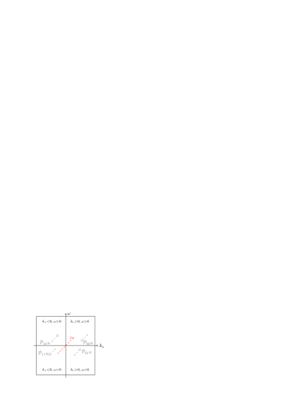
Figure 1: Forward- and backward propagating waves in $\{k_{z},\omega\}$-plane identified by the projectors $\hat{\mathcal{P}}_{lm}$ [Eq. (17)]. Arrows parallel to $z$-axis show the propagation direction of each type of waves.

The projector $\hat{\mathcal{P}}_{00}$ cuts off the part of the spectrum of $u$ that does not belong to the quadrant $k_{z}>0$, $\omega>0$ (i.e., it keeps only the upper right quadrant in the $\{k_{z},\omega\}$-plane, see Fig. 1). Similarly, $\hat{\mathcal{P}}_{01}$ only keeps the right lower quadrant, $\hat{\mathcal{P}}_{01}$ filters the left upper quadrant and $\hat{\mathcal{P}}_{11}$ the left lower quadrant of the $\{k_{z},\omega\}$-plane. It is easy to see that, according to Eq. (14), the border values $k_{z}=0$ or $\omega=0$ make an equal impact to both forward- and backward-propagating waves. This property formally follows from our definition of $\Theta$ in Eq. (14), which maps the point $0$ to $1/2$ at the frontiers of two quadrants. This is intuitively reasonable, because for waves propagating exactly perpendicularly to the $z$-axis, one cannot decide whether they propagate forward or backward along $z$. Obviously, all the operators defined above are continuous and linear, and they possess the property

$$\hat{\mathcal{P}}_{l}^{2}=\hat{\mathcal{P}}_{l},\,l=\pm,z\pm;\;\hat{\mathcal{P}}_{lm}^{2}=\hat{\mathcal{P}}_{lm},\,l,m=0,1,$$ (20)

which is common to projecting operators.

Definition III.2.

A tempered distribution $u\in\mathscr{S}^{\prime}(\mathbb{R}^{3}\times\mathbb{R})$, $u\neq 0$, is called forward- (backward-) propagating in $z$-direction or $z$-propagating iff $\hat{\mathcal{P}}_{+}u=u$ ($\hat{\mathcal{P}}_{-}u=u$).

Equipped with these definitions we can formulate the following result:

Lemma III.3.

An arbitrary $u(\mathrm{\mathbf{r}},t)\in\mathscr{S}^{\prime}(\mathbb{R}^{3}\times\mathbb{R})$ can be decomposed into the sum of forward- and backward- $z$-propagating functions.

From Def. III.1 we easily see that $\hat{P}_{+}+\hat{P}_{-}=\hat{I}$, where $\hat{I}$ is a unit operator. Thus, $u=\hat{P}_{+}u+\hat{P}_{-}u$.

It should be noted that the decomposition defined by lemma III.3 is not unique, since we can prescribe both forward- and backward- directions to the components of $u$ with $\left.\mathcal{F}\left[u\right](\mathrm{\mathbf{k}},\omega)\right|_{k_{z}=0}$, $\left.\mathcal{F}\left[u\right](\mathrm{\mathbf{k}},\omega)\right|_{\omega=0}$. Nevertheless, for the subspace $\{u\in\mathscr{S}^{\prime}(\mathbb{R}^{3}\times\mathbb{R}):\mathcal{F}[u]_{k_{z}=0}=0,\,\mathcal{F}[u]_{\omega=0}=0\}$, the decomposition is, indeed, unique.

Definition III.4.

The action of the projectors $\hat{\mathcal{P}}_{lm}$, $\hat{\mathcal{P_{\pm}}}$, $\hat{\mathcal{P}}_{z\pm}$ is defined as follows:

$$\forall(u,\phi)\in\mathscr{S}^{\prime}(\mathbb{R}^{3}\times\mathbb{R})\times\mathscr{S}(\mathbb{R}^{3}\times\mathbb{R}),$$

$$\langle u,\hat{\mathcal{P}}_{m}\phi\rangle=\langle\hat{\mathcal{P}}_{m}u,\phi\rangle,\,m=\pm,z\pm,\,\langle u,\hat{\mathcal{P}}_{lm}\phi\rangle=\langle\hat{\mathcal{P}}_{lm}u,\phi\rangle,\,l,m=0,1.$$ (21)

By virtue of the Plancherel’s relation (12), we deduce that $\hat{\mathcal{P}}_{\pm}$, $\hat{\mathcal{P}}_{z\pm}$, and $\hat{\mathcal{P}}_{lm}$, applied to tempered distributions, filter the corresponding regions in Fourier domain as well.

Remark III.5.

The fundamental solutions $\mathcal{E}_{\square\pm}$ of the wave equation (7) contain components propagating both forward and backward in $z$.

This can be seen by performing the temporal Fourier transform of Eq. (7), that expresses as $-e^{\pm i\omega r/c}/(4\pi r)$. This expression is indeed invariant when reverting the sign of $z$, therefore its Fourier transform must contain components both with $k_{z}>0$ and $k_{z}<0$ for every $\omega$.

IV The Fundamental Solution for the UPPE (4)

Now, equipped with the definitions in Sec. II, III, we can formulate our main result:

Theorem IV.1.

The fundamental solution $\mathcal{E}\in\mathscr{S}^{\prime}(\mathbb{R}^{3}\times\mathbb{R})$ of Eq. (4) exists and can be represented as

$$\mathcal{E}=\Theta(z)\hat{\mathcal{P}}_{z+}\left\{\mathcal{E}_{\square+}+\mathcal{E}_{\square-}\right\},$$ (22)

where $\mathcal{E}_{\square\pm}$, $\mathcal{P}_{z+}$ and $\Theta(z)$ are given by Eq. (7), Eq. (19) and Eq. (14), respectively.

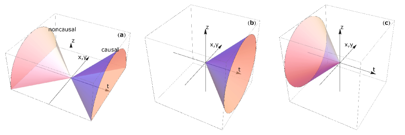
Figure 2: (a) Visual representation of the fundamental solution $\mathcal{E}$ defined by Eq. (22) projected to the $\{t,x\,\mbox{or}\,y,z\}$ plane. In (b), (c), the fundamental solutions of the wave equation (1), $\mathcal{E}_{\square+}$ and $\mathcal{E}_{\square-}$, are given for comparison [cf. Eq. (7)]. Only one of these, namely $\mathcal{E}_{\square+}$ in (b), fully respects the causality principle. In all other cases the waves, describing the response to an elementary excitation, appear before the excitation itself, i.e., $\mathcal{E}$ contains components propagating both forward and backward in time (see the causal and noncausal zones of half-cones, respectively).

Before we proceed with the proof of this theorem, a few remarks are needed. The fundamental solution given by Eq. (22) is visualized in Fig. 2. For $z>0,t>0$, it coincides with $\mathcal{E}_{\square+}$ and for $z>0,t<0$ with $\mathcal{E}_{\square-}$. Nevertheless, two features making it different from the fundamental solution of the wave equation (1) can be immediately seen:

Remark IV.2.

In contrast to the two fundamental solutions of the wave equation $\mathcal{E}_{\square\pm}$, the fundamental solution $\mathcal{E}$ of the UPPE extends in both directions in time.

We also notice that the projector $\hat{\mathcal{P}}_{z+}$ ($\hat{\mathcal{P}}_{z-}$) does not allow to select the set of only forward-propagating functions (resp., only backward-propagating functions). Thus, taking into account the Remark III.5 we can conclude that:

Remark IV.3.

The fundamental solution of the UPPE (22) contains components propagating both forward and backward in $z$.

The rest of the section is a technical proof of Theorem IV.1. We proceed by solving Eq. (2), the Fourier-transformed analog of Eq. (4) for $Q=\delta(z)$ [note that Eq. (13) is written in $\{k_{x},k_{y},z,\omega\}$ space, so that $\mathcal{F}_{\mathrm{\mathbf{r}}_{\bot},t}\left[\delta(\mathrm{\mathbf{r}},t)\right]=\delta(z)$]. As it is known (see for example Vladimirov (1976)) the fundamental solution of the operator $\frac{d}{dz}+a$ for any $a\in\mathbb{C}$ exists and is given by the expression $\Theta(z)e^{-az}$. Thus, the fundamental solution $\mathcal{E}$ of Eq. (4) exists and belongs to $\mathscr{S}^{\prime}(\mathbb{R}^{3}\times\mathbb{R})$, such as

$$\mathcal{E}(\mathrm{\mathbf{r}},t)=\Theta(z)\mathcal{F}_{\mathrm{\mathbf{k}}_{\bot},\omega}^{-1}\left[\frac{\exp(i\beta_{z}z)}{2i\beta_{z}}\right].$$ (23)

We will also use the following relation:

$$\exp(i\beta_{z}z)=\lim_{\epsilon\to 0}-i\mathcal{F}_{k_{z}}^{-1}\left[\left\{\frac{1}{k_{z}-\beta_{z}-i\epsilon}-\frac{1}{k_{z}-\beta_{z}+i\epsilon}\right\}\right].$$ (24)

Equation (24) must be understood in the sense of distributions: It follows directly from Sokhotsky’s formulas $\lim_{\epsilon\to 0}1/(x\pm i\epsilon)=\mp i\pi\delta(0)+\mathscr{P}(1/x)$, where the Cauchy principal value is defined by

$$\langle\mathscr{P}(1/x),f(x)\rangle=\lim_{\epsilon\to 0}(\int_{-\infty}^{-\epsilon}+\int_{+\epsilon}^{+\infty})\frac{f(x)}{x}dx,$$ (25)

$\forall f\in\mathscr{S}(\mathbb{R}^{3}\times\mathbb{R})$. In addition, taking into account that $k_{z}^{2}+\beta_{z}^{2}=k^{2}+\beta^{2}$ (where $\mathrm{\mathbf{k}}=\{\mathrm{\mathbf{k}}_{\bot},k_{z}\}$, $k^{2}=k_{z}^{2}+k_{\bot}^{2}$, $\beta=\omega/c$), the expressions $1/(k_{z}-\beta_{z}\pm i\epsilon)$ can be rewritten in the limit $\epsilon\rightarrow 0$ as:

$$\frac{\pm 1}{k_{z}-\beta_{z}\mp i\epsilon}=\pm\frac{k_{z}+\beta_{z}}{k^{2}-\beta^{2}\mp i\epsilon}=\pm\frac{k_{z}+\beta_{z}}{k^{2}-(\beta\pm i\epsilon\operatorname{sign}\beta)^{2}}.$$ (26)

Substituting Eq. (24), Eq. (26) into Eq. (23) and decomposing the resulting expression into parts corresponding to the summands in Eq. (26), we then get

$$\mathcal{E}\equiv\Theta(z)(\mathcal{E}_{+}+\mathcal{E}_{-});\,\mathcal{E}_{\pm}=\pm\lim_{\epsilon\to 0}\mathcal{F}^{-1}\left[\frac{k_{z}+\beta_{z}}{2\beta_{z}}\frac{1}{k^{2}-(\beta\mp i\epsilon\operatorname{sign}\beta)^{2}}\right].$$ (27)

We can explicitly perform the Fourier transform $\mathcal{F}^{-1}_{\omega}$, that is, integrate over $\omega$ to obtain

$$\mathcal{E}_{\pm}=\pm\frac{ic}{2}\mathcal{F}^{-1}_{k_{x},k_{y},k_{z}}\left[\Theta(k_{z})\frac{e^{\mp ickt}}{k}\right].$$ (28)

$\Theta(k_{z})$ appears because the integration over $\omega$ gives $\beta_{z}\to|k_{z}|$ and thus $k_{z}+\beta_{z}\to k_{z}+|k_{z}|=2\Theta(k_{z})|k_{z}|$. Taking into account that $\mathcal{E}_{\square\pm}$ can be rewritten as Jackson (1962)

$$\mathcal{E}_{\square\pm}=-c\Theta(\pm t)\mathcal{F}^{-1}_{k_{x},k_{y},k_{z}}\left[\frac{\sin{(ckt)}}{k}\right]$$ (29)

and using Eq. (27) finally leads to Eq. (22).

V the UPPE with Paraxial Nonlinearity

The UPPE in Eq. (4) is free from paraxial approximation, i.e., no assumption is applied to the ratio $k_{z}/k$ allowed in the solution. However, for practical uses, Kolesik and Moloney (2004); Babushkin et al. (2010); Bergé et al. (2013) a simplified, but computationally more performing variant of the UPPE may be employed, namely,

$$\partial_{z}E-i\Phi\star E=\frac{1}{2i}\Psi^{\prime}\star Q,$$ (30)

where

$$\Psi^{\prime}=\mathcal{F}_{\{k_{x},k_{y},\omega\}}^{-1}[1/|\beta|],$$ (31)

i.e., $\beta_{z}$ is replaced by $|\beta|$ in the denominator of the right-hand side of Eqs. (4), (5). This equation can be obtained using the well-known paraxial approximation $ck_{\bot}/\omega\ll 1$ in the inhomogeneous term of Eq. (4). This amounts to considering that the transverse spatial components of the field are large in front of its central wavelength. Under these conditions we can omit the diffraction wave numbers in the square root $\beta_{z}=\sqrt{\omega^{2}/c^{2}-k_{\bot}^{2}}$ affecting the inhomogeneity $Q$, thus replacing there $\beta_{z}$ by $|\beta|=|\omega/c|$.

Definition V.1.

Equation (30) is called the paraxial UPPE.

Theorem V.2.

The fundamental solution $\mathcal{E}_{p}\in\mathscr{S}^{\prime}(\mathbb{R}^{3}\times\mathbb{R})$ of Eq. (30) exists and expresses as

$$\mathcal{E}_{p}=c\Theta{(z)}\int_{-\infty}^{t}\partial_{z}\left\{\mathcal{E}_{-}-\mathcal{E}_{+}\right\}\,d\tau,$$ (32)

where $\mathcal{E}_{\pm}$ are given by Eq. (27).

Proceeding as in the previous section, we introduce $\mathcal{E}_{p\pm}$ similarly to Eq. (27), so that

$$\mathcal{E}_{p}=\Theta(z)(\mathcal{E}_{p+}+\mathcal{E}_{p-}),$$ (33)

$$\mathcal{E}_{p\pm}=\mathcal{F}^{-1}\left[\frac{\beta_{z}}{|\beta|}\tilde{\mathcal{E}}_{\pm}\right],$$ (34)

where

$$\tilde{\mathcal{E}}_{\pm}=\frac{\pm 1}{k^{2}-(\beta\mp i\epsilon\operatorname{sign}\beta)^{2}}\frac{k_{z}+\beta_{z}}{2\beta_{z}}.$$ (35)

The formula for $\mathcal{E}_{p\pm}$ is different from Eq. (27) by the factor $\beta_{z}/|\beta|$. Analogously to Eq. (28), the above equation can be transformed into

$$\mathcal{E}_{p\pm}=\pm\frac{ic}{2}\mathcal{F}^{-1}_{k_{x},k_{y},k_{z}}\left[\Theta(k_{z})\frac{e^{\mp ickt}}{k}\frac{k_{z}}{k}\right].$$ (36)

In Eq. (36) we took into account that $|k|=k$ since $k\geq 0$ and $|k_{z}|\Theta(k_{z})=k_{z}\Theta(k_{z})$. This equation can be re-expressed in $\{\mathrm{\mathbf{r}},t\}$-space as

$$\mathcal{E}_{p\pm}=\mp c\int_{-\infty}^{t}\partial_{z}\mathcal{E}_{\pm}\,d\tau,$$ (37)

which finally results in Eq. (32).

VI Conclusions

In summary, although in the 3-dimensional UPPE (2) the “selected axis” $z$ is pre-imposed, it enters UPPE solutions in a way, which, in many respects, remains similar to that in the solutions to the 3-dimensional wave equation (1). In particular, an inhomogeneity in the form of $\delta$-function in UPPE produces wave solutions propagating both forward and backward in $z$-direction and in time, as formulated by Eq. (22), Remarks IV.2 and IV.3. This may sound in contradiction with the commonly-used name “unidirectional” given to this equation. However, if the excitation $Q$ is a forward- or backward-propagating function, that is $Q=\hat{\mathcal{P}}_{\pm}Q$, the field created by this excitation and given by $\mathcal{E}\star Q$ is also forward- or backward-propagating, since $\mathcal{E}\star Q=\mathcal{E}\star\hat{\mathcal{P}}_{\pm}Q=\hat{\mathcal{P}}_{\pm}(\mathcal{E}\star Q)$ by virtue of Eq. (22). Hence, reframed in its original context for which $Q$ is a nonlinear function of $E$, it is important that the nonlinearity $Q$ be modeled in such a way that it does not create backward fields.

Strictly speaking, the fact that the inhomogeneity $Q$ excites waves which propagate in both directions in time breaks the causality principle. As illustrated in Fig. 2, the wave created by the excitation ($\delta$-function) can propagate both forward and backward in time, which means that an observer could see the result of the excitation before the latter be triggered. This is prohibited by the causality principle, and, therefore, further studies should attempt to cure this point for a better physical description of wave propagation.

Finally, another important feature related to the number of spatial dimensions can also be inferred from our analysis. By assuming a source created by a plasma current $J$ near some spatial point $\mathrm{\mathbf{r}}_{0}$, the radiated field solution will be given by $E\,\sim\,Q\propto\partial_{t}J$ in the framework of the three-dimensional ($\{x,y,z\}$) wave equation. Our results suggest that, up to the functional projector $\mathcal{P}_{z+}$, the basic proportionality $E\sim\partial_{t}J$ holds for the UPPE (4). In contrast, the paraxial UPPE (30) would rather support the relationship $E\sim\partial_{z}J$. For comparison, the 1D ($\{z\}$) wave equation, whose elementary solutions express as $\mathcal{E}_{\square\pm}\propto\Theta(t\mp|z|/c)$ (see, for example Vladimirov (1976)), would promote a radiated field solution proportional to $J$ directly, i.e., $E\sim J$, since the Heaviside function assures a pre-integration in time ($\partial_{t}\Theta=\delta$).