Three Dimensional Edwards-Anderson Spin Glass Model in an External Field

Abstract

We study the Edwards-Anderson model on a simple cubic lattice with a finite constant external field. We employ an indicator composed of a ratio of susceptibilities at finite wavenumbers, which was recently proposed to avoid the difficulties of a zero momentum quantity, for capturing the spin glass phase transition. Unfortunately, this new indicator is fairly noisy, so a large pool of samples at low temperature and small external field are needed to generate results with sufficiently small statistical error for analysis. We thus implement the Monte Carlo method using graphics processing units to drastically speedup the simulation. We confirm previous findings that conventional indicators for the spin glass transition, including the Binder ratio and the correlation length do not show any indication of a transition for rather low temperatures. However, the ratio of spin glass susceptibilities do show crossing behavior, albeit a systematic analysis is beyond the reach of the present data. This calls for a more thorough study of the three dimensional Edwards-Anderson model in an external field.

Introduction. Most spin systems order when the temperature is sufficiently low. Conventional magnetic orderings break spin symmetry, and the moments align in a pattern with long range order. However, magnetic systems with random frustrated couplings can avoid conventional ordering by breaking ergodicity. Typical spin glass systems with such competing magnetic couplings include localized spins in metals coupled via the oscillating Rudermann-Kittel-Kasuya-Yoshida exchange as CuFe and CuMn, and in insulators with competing interactions as in LiHoYF and EuSrS Binder and Young (1986); Mydosh (1993); Diep (2004). These systems do not display long range order for a wide range of diluted spin concentrations.

A widely studied model to describe spin glass physics is the Edwards-Anderson (EA) modelEdwards and Anderson (1975). It is composed of spins interacting with their nearest neighbors via random couplings. The mean-field variant of the EA model, the Sherrington-Kirkpatrick (SK) modelKirkpatrick and Sherrington (1978); Sherrington and Kirkpatrick (1975), was solved by the replica technique in 1975 with the striking observation that the entropy can be negative at low temperatureSherrington and Kirkpatrick (1975); Kirkpatrick and Sherrington (1978). A cavity mean field method was proposed by Thouless, Anderson and Palmer (TAP) in which the local magnetization of each site is considered as an independent order parameterThouless et al. (1977). The hope was to obtain a more physical mean field solution without involving the replica technique. However, multiple solutions were foundBray and Moore (1980).

Motivated by the deficits of previous approaches, de Almedia and Thouless further studied the replica symmetric mean field solution and found a line in the temperature–magnetic field plane where the replica symmetry solution is unstable towards replica symmetry breaking (RSB) de Almeida and Thouless (1978). The replica overlap has more structure than simply a constant. The way to characterize this structure for a stable mean field solution was developed by Parisi Parisi (1980b, a, c). There is a hierarchy of the replica overlap, and this can be described in terms of a ultra-metric tree. The replica symmetry breaking scheme resolved the negative entropy crisis and naturally explained the many solutions found in the TAP approach.

The RSB theory is accepted to be the correct description of the SK model, indeed it provides the exact free energy Talagrand (2006); Guerra (2003). However, its applicability to real spin glasses has been intensively debated over the last three decades, especially in the three dimensions case. For systems below the upper critical dimension Harris et al. (1976); Tasaki (1989); Green et al. (1983) the most prominent competing theory is the droplet model elaborated by Huse and Fisher Fisher and Huse (1988, 1987) and based on the idea of domain wall scaling by Moore, Bray and McMillan McMillan (1984); Bray and Moore (1987). In this theory, there exists a finite characteristic length scale where droplets of excitations can loose energy by aligning with the field. The spin glass phase is thus destroyed by any finite external field. Moreover, those excitations are assumed to be compact and with fractal dimension smaller than the spacial dimension, in contrast with the space-filling excitations in the mean field theory.

Thus a possible scheme to discern between the RSB and the droplet theories is to determine whether a spin glass phase exists at a finite external field Young and Katzgraber (2004). There are other schemes based on the differences in the overlap and the excitations in these two theories. For example, the distribution of the overlap and parameters that characterize it Hatano and Gubernatis (2002); Marinari et al. (1998, 1999); Bokil et al. (1999); Moore et al. (1998); Monthus and Garel (2013), the existence of the ultra-metric structure in the overlap Hed et al. (2004); Contucci et al. (2007), and the nature of the ground state and its excitations Palassini and Young (2000a, b); Aspelmeier et al. (2003); Marinari and Parisi (2001); Houdayer and Martin (1999); Marinari et al. (2000, 1999). Unfortunately, the conclusions draw from different studies are often controversial. This is mostly due to two factors, the limitation in the system sizes that can be simulated and the interpretation of the data.

Using the same techniques on the three dimensional EA model under an external field, no signal of a crossing of the scaled correlation length for different system sizes can be detectedYoung and Katzgraber (2004). We will show this is also the case for the Binder ratio. The absence of crossing is a powerful evidence that a spin glass phase is absent in the presence of an external field. However, it has been argued that the system sizes studied may be too small and far from the scaling regime. To remedy this problem, one dimensional models with long range power-law decaying interactions Kotliar et al. (1983) which mimic the short range models at higher dimensions have been intensively studied over last few years Katzgraber and Young (2003b, a); Leuzzi (1999). In these models much larger systems can be studied Katzgraber et al. (2009); Katzgraber and Hartmann (2009); Leuzzi et al. (2008); Larson et al. (2013).

On top of these controversies, it has been recently argued that the scaled correlation length is not a good parameter for the spin glass transition in a field since its calculation involves the susceptibility at zero momentum Leuzzi et al. (2008). The latest proposal is to study the ratio of susceptibilities at the two smallest non-zero momenta, denoted it as $R_{12}$ Baños et al. (2012). It has been shown that in four dimensions this quantity displays a crossing at finite temperature which is an important clue that the spin glass can still exist without time reversal symmetry below the upper critical dimension Baños et al. (2012). Giving the success of using $R_{12}$ to capture the spin glass phase at four dimensions, we reexamine the three dimensional EA model on a simple cubic lattice using a new development in computer architecture, and the recently proposed $R_{12}$. We will demonstrate that graphic card computing is particularly well suited for equilibrium simulations of spin glass systems, in particular for cases where a huge number of realizations is required such as the model we study in this work.

Methods and Measured Quantities. The Hamiltonian for the EA model is given as

$$H=-\sum_{<i,j>}J_{ij}S_{i}S_{j}-h\sum_{i}S_{i},$$ (1)

where $S_{i}$ indicate Ising spins on a simple cubic lattice with $N=L^{3}$ sites and periodic boundary conditions. The coupling $J_{ij}$ is bimodal distributed with probability $P(J_{ij})=\frac{1}{2}(\delta(J_{ij}-1)+\delta(J_{ij}+1))$, and $h$ is an external field.

The spin glass overlap is defined as

$$q(\mathbf{k})=\frac{1}{N}\sum_{j}S_{j}^{(\alpha)}S_{j}^{(\beta)}\exp^{i\mathbf{k}\cdot\mathbf{r}_{j}},$$ (2)

where $\alpha$ and $\beta$ are two independent realizations of the same disorder model. We calculate the overlap kurtosis or the Binder ratio from the overlap as Ciria et al. (1993); Marinari et al. (1998)

$$g=\frac{1}{2}\left(3-\frac{\overline{\left<\left(q(0)-\overline{\left<q(0)\right>}\right)^{4}\right>}}{\overline{\left<\left(q(0)-\overline{\left<q(0)\right>}\right)^{2}\right>}^{2}}\right).$$ (3)

Note that $\overline{(\cdots)}$ indicates averaging over different disorder realizations, and $\left<\cdots\right>$ denotes thermal averaging.

The wave vector dependent spin glass susceptibility is defined as Marinari et al. (1998)

$$\chi(\mathbf{k})=N(\overline{\left<q^{2}(\mathbf{k})\right>}-\overline{\left<q(\mathbf{k})\right>}^{2}),$$ (4)

and the correlation length as

$$\xi_{L}=\frac{1}{2\sin(\mathbf{k}_{\mathrm{min}}/2)}\left[\frac{\chi(0)}{\chi(\mathbf{k}_{\mathrm{min}})}-1\right]^{1/2},$$ (5)

where $\mathbf{k}_{\mathrm{min}}=(2\pi/L,0,0)$.

We define $R_{12}$ as the ratio between the susceptibilities with the two smallest non-zero wave vectors Baños et al. (2012)

$$R_{12}=\frac{\chi(\mathbf{k}_{1})}{\chi(\mathbf{k}_{2})},$$ (6)

where $\mathbf{k}_{1}=(2\pi/L,0,0)$, $\mathbf{k}_{2}=(2\pi/L,2\pi/L,0)$.

Parallel temperingHukushima and Nemoto (1996); Marinari and Parisi (1992) is used to accelerated the thermalization, in which $N_{T}$ samples of the same disorder coupling are simulated in parallel within a range of temperatures. In order to compute the spin glass overlap (Eq.2) we simulate two replicas of the system with the same bonds $J_{ij}=\pm 1$ and field $h$ at each temperature.

We implement the Monte Carlo simulation with parallel tempering on graphics processing units using the CUDA programming language Nickolls et al. (2008). Multispin codingCreutz et al. (1979); Zorn et al. (1981) is used to pack the $N_{T}$ replicas into the small but extremely fast shared memory. We achieve a performance of 33ps per spin flip attempt on a GTX 580 card. We use the CURAND implemented XORWOW generator to generate random numbers NVIDIA (2010). Since the GPU is a commodity hardware and widely available in large computer clusters, it is now easy to greatly accelerate these simulations. The details of the implementation can be found in Ref Fang et al., 2013.

Table 1: Parameters of the simulations. $L$ is the linear system size. $N_{\mathrm{samp}}$ is the number of samples, $N_{\mathrm{sweep}}$ is the total number of Monte Carlo sweeps for each of the 2$N_{T}$ replicas for a single sample, $\beta_{\mathrm{max}}$ and $\beta_{\mathrm{min}}$ shows the temperature region simulated, and $N_{T}$ is the number of temperatures used in the parallel tempering method. The temperature set in each simulation follows a geometric distribution, i.e. $\beta_{n}=\beta_{\rm min}\alpha^{n-1}$, where $\alpha=(\beta_{\rm max}/\beta_{\rm min})^{1/(N_{T}-1)}$, $n\in[1,N_{T}]$. The first half of the Monte Carlo sweeps are used for thermalization and the second half are used for measurement.

$L$	$N_{\mathrm{samp}}$	$N_{\mathrm{sweep}}$	$N_{T}$	$\beta_{\mathrm{max}}$	$\beta_{\mathrm{min}}$
6	500,000	2,000,000	56	1.8	0.1
8	350,000	2,000,000	56	1.8	0.1
10	240,000	2,000,000	56	1.8	0.1

We list the parameters of our simulation in Table 1. We benchmarked the code against existing results at $h=0$. The smallest $\beta$ used in the parallel tempering is well below the critical temperature ($1/\beta_{c}=T_{c}\approx 1.1019\pm 0.0029$) Baity-Jesi et al. (2013) of the spin glass transition at zero fieldBallesteros et al. (2000); Baity-Jesi et al. (2013), while the largest $\beta$ is about two times larger. The estimated critical field at zero temperature is around $h\approx 0.65$ for the model with zero mean and unit variance Gaussian distributed couplingsKrzakala et al. (2001). We choose to work in a relatively small field, $h=0.1$. The jackknife method is used to estimate the statistical errors from disorder averaging.

Results. We plot the spin glass susceptibility in Fig. 1. As in the zero field case, the susceptibility increases as the temperature is lowered, however there is no obvious asymptotic scaling behavior. In particular, for temperatures below the zero-field critical temperature, the slope of the curves decreases and they begin to bend downward. This result is similar to the one obtained for the one dimensional modelLarson et al. (2013), but in contrast with the results of the four dimensional lattice which displays asymptotic divergent susceptibilities Marinari et al. (1998).

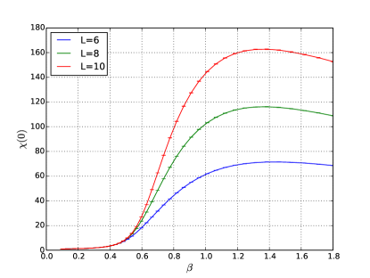
Figure 1: Spin glass susceptibility at zero momentum, $\chi(0)$, as a function of inverse temperature for system sizes $L=6,8,10$.

As the susceptibility does not show a behavior in accordance with the conventional finite size scaling theory for a second order transition, we move to study various cumulants and ratios of susceptibilities of the overlap parameter. We show the Binder ratio in the Fig. 2. It does not display any signal of crossing. Indeed, the curves for different system sizes do not even tend to merge as the temperature is lowered. Note that the Binder ratio corresponds to the fourth-order cumulant of the distribution, and the possible issues related with the soft mode contributing to the zero momentum susceptibility should likely be canceled in the Binder ratio.

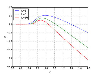
Figure 2: Binder ratio as a function of inverse temperature in the range $\beta=0.1\sim 1.8$ for system sizes $L=6,8,10$.

Fig. 3 displays the scaled correlation length. This is now a standard diagnosis for the detection of a spin glass transition. The correlation length is extracted from the Ornstein-Zernike form (Eq. 5), and thus essentially given by the ratio between the zero and the smallest finite momentum susceptibilities. Similar to the Binder ratio, and consistent with other results in the literature, there is no crossing or even merging down to a rather low temperature Young and Katzgraber (2004).

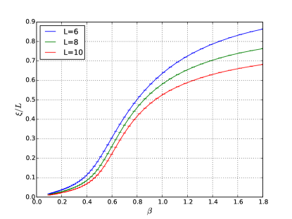
Figure 3: Scaled correlation length $\xi/L$ as a function of inverse temperature for system sizes $L=6,8,10$.

From now on we focus on $R_{12}$. We first perform simulations in zero field where $R_{12}$ shows a crossing close to the expected critical temperature found from the Binder ratio and the correlation length. Therefore, the crossing in $R_{12}$ should be a viable indicator for the phase transition. Unfortunately, we find that $R_{12}$ is in general much nosier than other quantities. This is due to the fact that the sampling of higher momentum quantities is almost always characterized by larger statistical fluctuations. Taking the ratio between two susceptibilities at finite momenta clearly further harms the quality of the data. To reduce the error bars we generate long runs and larger pools of disorder realizations (see Table 1). This is the main reason we have generated a rather large number ($2.4\times 10^{5}$) of realizations for the largest systems size we present here, and even more for smaller sizes. To further reduce the fluctuations, we impose all point group symmetries. For example, when we calculate $\chi(2\pi/L,0,0)$ we average the susceptibility at three different directions ($\chi(2\pi/L,0,0)$, $\chi(0,2\pi/L,0)$, and $\chi(0,0,2\pi/L)$). This averaging implicitly assumes that the point group symmetry is restored which is justified only when the number of realization is rather large.

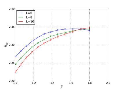
Figure 4: $R_{12}$ as a function of inverse temperature for different system sizes. An intersection can be seen at around $T\approx 0.6$. We use the jackknife method to estimate the error bar from sample-to-sample variation.

Fig. 4 displays $R_{12}$. In contrast to other quantities, $R_{12}$ shows an intersection at about $T\approx 0.6$. We do not think we have sufficient data to perform a reasonably accurate finite size scaling analysis to report the exponent or even to quantify the correction. Hasenbusch et al. (2008) Moreover, the data for $L=6$ does not seem to fit into a finite size scaling form with the curve bending downward. Unfortunately, parallel tempering Monte Carlo is not robust enough for simulating larger lattices in a reasonable amount of time, this can be related to the temperature chaos Ritort (1994); Fernandez et al. (2013); Katzgraber and Krza¸kała (2007). The number of replicas needed to equilibrate the system also increases substantially as the system size increases, we already used $56$ temperature replicas for $L=10$ simulations. We plot $R_{12}$ versus the number of Monte Carlo sweeps in Fig. 5. We believe the data is sufficiently equilibrated for averaged quantities. The major contribution to the error is from the limited number of disorder realizations. Fig. 6 shows $R_{12}$ for $L=10$ and different number of realizations. We clearly see that the data converges only when the number of realizations is fairly large. This is one of the prominent hurdles of using higher momentum susceptibility as a diagnosis. We note that the effective one dimensional model also shows crossing behavior, albeit the crossing points do not show a systematic trendLarson et al. (2013).

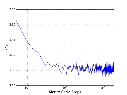
Figure 5: $R_{12}$ for $L=10$ at $\beta=1.8$, as a function of the number of Monte Carlo sweeps. We believe the averaged data is equilibrated for $10^{6}$ sweeps, and it passes the logarithm binning test Baños et al. (2010). The main contribution to the error is from the realization averaging.

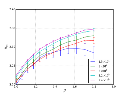
Figure 6: $R_{12}$ for $L=10$ and low temperatures ($\beta\geq 1.0$). We show five different number of realizations from fifteen thousands to two-hundreds forty thousands.

Conclusion. In summary, we perform Monte Carlo simulations of the three dimensional Edwards-Anderson model in a finite external field. The goal is to reexamine the long standing problem whether mean field behavior, specifically a spin glass phase, can exist in such a model without time-reversal symmetry. We focus on the equilibrium quantities of this notoriously difficult system. By taking advantage of the new commodity multi-threaded graphic computing units architecture we drastically reduce the computation time. The results for the Binder ratio and correlation length show no signal of intersection, thus they point to the absence of spin glass transition according to conventional wisdom. On the other hand, the ratio of susceptibilities $R_{12}$ does show crossing behavior for relatively small system sizes ($L=6,8,10$). We did perform simulations for larger system sizes, but we are not confident that those simulations reach equilibrium since the data is too noisy in particular for $R_{12}$. With the present system sizes and the statistical error bar, a rigorous data analysis does not seem to deliver unbiased information. This situation is rather discouraging, as simulations at this low temperature for much large system sizes using the present method are daunting. This calls for a more thorough study on the model with different approaches. Possible directions include: 1) using models with continuous random distribution which are easier to thermalize than that with bimodal distribution; 2) analyzing the data for the distribution of the overlap parameter, instead of average quantities. We notice a preprint before we finished the present paper where the conditioning variate method is used to expose the silent features from the data Baity-Jesi et al. (2014).

This work is sponsored by the NSF EPSCoR Cooperative Agreement No. EPS-1003897 with additional support from the Louisiana Board of Regents. Portions of this research were conducted with high performance computational resources provided by Louisiana State University (http://www.hpc.lsu.edu). We thank Helmut Katzgraber and Karen Tomko for useful conversations.

References

- Binder and Young (1986) K. Binder and A. P. Young, Rev. Mod. Phys. 58, 801 (1986).
- Diep (2004) H. Diep, Frustrated Spin Systems (World Scientific, 2004).
- Mydosh (1993) J. Mydosh, Spin Glasses: An Experimental Introduction (Taylor & Francis Group, 1993).
- Edwards and Anderson (1975) S. F. Edwards and P. W. Anderson, Journal of Physics F: Metal Physics 5, 965 (1975).
- Kirkpatrick and Sherrington (1978) S. Kirkpatrick and D. Sherrington, Phys. Rev. B 17, 4384 (1978).
- Sherrington and Kirkpatrick (1975) D. Sherrington and S. Kirkpatrick, Phys. Rev. Lett. 35, 1792 (1975).
- Thouless et al. (1977) D. Thouless, P. Anderson, and R. Palmer, Philosophical Magazine 35, 593 (1977).
- Bray and Moore (1980) A. J. Bray and M. A. Moore, Journal of Physics C: Solid State Physics 13, L469 (1980).
- de Almeida and Thouless (1978) J. R. L. de Almeida and D. J. Thouless, Journal of Physics A: Mathematical and General 11, 983 (1978).
- Parisi (1980a) G. Parisi, Journal of Physics A: Mathematical and General 13, 1887 (1980a).
- Parisi (1980b) G. Parisi, Journal of Physics A: Mathematical and General 13, 1101 (1980b).
- Parisi (1980c) G. Parisi, Journal of Physics A: Mathematical and General 13, L115 (1980c).
- Guerra (2003) F. Guerra, Communications in Mathematical Physics 233, 1 (2003).
- Talagrand (2006) M. Talagrand, Annals of Mathematics 163, pp. 221 (2006).
- Green et al. (1983) J. E. Green, M. A. Moore, and A. J. Bray, Journal of Physics C: Solid State Physics 16, L815 (1983).
- Harris et al. (1976) A. B. Harris, T. C. Lubensky, and J.-H. Chen, Phys. Rev. Lett. 36, 415 (1976).
- Tasaki (1989) H. Tasaki, Journal of Statistical Physics 54, 163 (1989).
- Fisher and Huse (1987) D. S. Fisher and D. A. Huse, Journal of Physics A: Mathematical and General 20, L1005 (1987).
- Fisher and Huse (1988) D. S. Fisher and D. A. Huse, Phys. Rev. B 38, 386 (1988).
- Bray and Moore (1987) A. Bray and M. Moore, in Heidelberg Colloquium on Glassy Dynamics, edited by J. Hemmen and I. Morgenstern (Springer Berlin Heidelberg, 1987), vol. 275 of Lecture Notes in Physics, pp. 121–153.
- McMillan (1984) W. L. McMillan, Journal of Physics C: Solid State Physics 17, 3179 (1984).
- Young and Katzgraber (2004) A. P. Young and H. G. Katzgraber, Phys. Rev. Lett. 93, 207203 (2004).
- Bokil et al. (1999) H. Bokil, A. J. Bray, B. Drossel, and M. A. Moore, Phys. Rev. Lett. 82, 5174 (1999).
- Hatano and Gubernatis (2002) N. Hatano and J. E. Gubernatis, Phys. Rev. B 66, 054437 (2002).
- Marinari et al. (1998) E. Marinari, C. Naitza, F. Zuliani, G. Parisi, M. Picco, and F. Ritort, Phys. Rev. Lett. 81, 1698 (1998).
- Marinari et al. (1999) E. Marinari, C. Naitza, F. Zuliani, G. Parisi, M. Picco, and F. Ritort, Phys. Rev. Lett. 82, 5175 (1999).
- Monthus and Garel (2013) C. Monthus and T. Garel, Phys. Rev. B 88, 134204 (2013).
- Moore et al. (1998) M. A. Moore, H. Bokil, and B. Drossel, Phys. Rev. Lett. 81, 4252 (1998).
- Contucci et al. (2007) P. Contucci, C. Giardinà, C. Giberti, G. Parisi, and C. Vernia, Phys. Rev. Lett. 99, 057206 (2007).
- Hed et al. (2004) G. Hed, A. P. Young, and E. Domany, Phys. Rev. Lett. 92, 157201 (2004).
- Aspelmeier et al. (2003) T. Aspelmeier, M. A. Moore, and A. P. Young, Phys. Rev. Lett. 90, 127202 (2003).
- Houdayer and Martin (1999) J. Houdayer and O. C. Martin, Phys. Rev. Lett. 82, 4934 (1999).
- Marinari et al. (2000) E. Marinari, G. Parisi, and F. Zuliani, Phys. Rev. Lett. 84, 1056 (2000).
- Marinari and Parisi (2001) E. Marinari and G. Parisi, Phys. Rev. Lett. 86, 3887 (2001).
- Palassini and Young (2000a) M. Palassini and A. P. Young, Phys. Rev. Lett. 85, 3017 (2000a).
- Palassini and Young (2000b) M. Palassini and A. P. Young, Phys. Rev. Lett. 85, 3333 (2000b).
- Kotliar et al. (1983) G. Kotliar, P. W. Anderson, and D. L. Stein, Phys. Rev. B 27, 602 (1983).
- Katzgraber and Young (2003a) H. G. Katzgraber and A. P. Young, Phys. Rev. B 68, 224408 (2003a).
- Katzgraber and Young (2003b) H. G. Katzgraber and A. P. Young, Phys. Rev. B 67, 134410 (2003b).
- Leuzzi (1999) L. Leuzzi, Journal of Physics A: Mathematical and General 32, 1417 (1999).
- Katzgraber and Hartmann (2009) H. G. Katzgraber and A. K. Hartmann, Phys. Rev. Lett. 102, 037207 (2009).
- Katzgraber et al. (2009) H. G. Katzgraber, D. Larson, and A. P. Young, Phys. Rev. Lett. 102, 177205 (2009).
- Larson et al. (2013) D. Larson, H. G. Katzgraber, M. A. Moore, and A. P. Young, Phys. Rev. B 87, 024414 (2013).
- Leuzzi et al. (2008) L. Leuzzi, G. Parisi, F. Ricci-Tersenghi, and J. J. Ruiz-Lorenzo, Phys. Rev. Lett. 101, 107203 (2008).
- Baños et al. (2012) R. A. Baños, A. Cruz, L. A. Fernandez, J. M. Gil-Narvion, A. Gordillo-Guerrero, M. Guidetti, D. Iñiguez, A. Maiorano, E. Marinari, V. Martin-Mayor, et al., Proceedings of the National Academy of Sciences 109, 6452 (2012).
- Ciria et al. (1993) J. C. Ciria, G. Parisi, F. Ritort, and J. J. Ruiz-Lorenzo, Journal de Physique I (France) 3, 2207 (1993).
- Hukushima and Nemoto (1996) K. Hukushima and K. Nemoto, Journal of the Physical Society of Japan 65, 1604 (1996).
- Marinari and Parisi (1992) E. Marinari and G. Parisi, Europhysics Letters 19, 451 (1992).
- Nickolls et al. (2008) J. Nickolls, I. Buck, M. Garland, and K. Skadron, Queue 6, 40 (2008).
- Creutz et al. (1979) M. Creutz, L. Jacobs, and C. Rebbi, Phys. Rev. Lett. 42, 1390 (1979).
- Zorn et al. (1981) R. Zorn, H. Herrmann, and C. Rebbi, Computer Physics Communications 23, 337 (1981).
- NVIDIA (2010) NVIDIA, CUDA CURAND Library, NVIDIA Corporation, Santa Clara, CA, USA (2010).
- Fang et al. (2013) Y. Fang, S. Feng, K.-M. Tam, Z. Yun, J. Moreno, J. Ramanujam, and M. Jarrell, ArXiv e-prints (2013), eprint 1311.5582.
- Ballesteros et al. (2000) H. G. Ballesteros, A. Cruz, L. A. Fernández, V. Martín-Mayor, J. Pech, J. J. Ruiz-Lorenzo, A. Tarancón, P. Téllez, C. L. Ullod, and C. Ungil, Phys. Rev. B 62, 14237 (2000).
- Baity-Jesi et al. (2013) M. Baity-Jesi, R. A. Baños, A. Cruz, L. A. Fernandez, J. M. Gil-Narvion, A. Gordillo-Guerrero, D. Iñiguez, A. Maiorano, F. Mantovani, E. Marinari, et al. (Janus Collaboration), Phys. Rev. B 88, 224416 (2013).
- Krzakala et al. (2001) F. Krzakala, J. Houdayer, E. Marinari, O. C. Martin, and G. Parisi, Phys. Rev. Lett. 87, 197204 (2001).
- Hasenbusch et al. (2008) M. Hasenbusch, A. Pelissetto, and E. Vicari, Phys. Rev. B 78, 214205 (2008).
- Ritort (1994) F. Ritort, Phys. Rev. B 50, 6844 (1994).
- Fernandez et al. (2013) L. A. Fernandez, V. Martin-Mayor, G. Parisi, and B. Seoane, EPL (Europhysics Letters) 103, 67003 (2013).
- Katzgraber and Krza¸kała (2007) H. G. Katzgraber and F. Krza¸kała, Phys. Rev. Lett. 98, 017201 (2007).
- Baños et al. (2010) R. A. Baños, A. Cruz, L. A. Fernandez, A. Gordillo-Guerrero, J. M. Gil-Narvion, M. Guidetti, A. Maiorano, F. Mantovani, E. Marinari, V. Martin-Mayor, et al., Journal of Statistical Mechanics: Theory and Experiment 2010, P05002 (2010).
- Baity-Jesi et al. (2014) M. Baity-Jesi, R. A. Baños, A. Cruz, L. A. Fernandez, J. M. Gil-Narvion, A. Gordillo-Guerrero, D. Iniguez, A. Maiorano, F. Mantovani, E. Marinari, et al., ArXiv e-prints (2014), eprint 1403.2622.