Coherent dynamics in long fluxonium qubits

Abstract

We analyze the coherent dynamics of a fluxonium device [V.E. Manucharyan et al., Science 326, 113 (2009)] formed by a superconducting ring of Josephson junctions in which strong quantum phase fluctuations are localized exclusively on a single weak element. In such a system, quantum phase tunnelling by $2\pi$ occurring at the weak element couples the states of the ring with supercurrents circulating in opposite directions, while the rest of the ring provides an intrinsic electromagnetic environment of the qubit. Taking into account the capacitive coupling between nearest neighbors and the capacitance to the ground, we show that the homogeneous part of the ring can sustain electrodynamic modes which couple to the two levels of the flux qubit. In particular, when the number of Josephson junctions is increased, several low-energy modes can have frequencies lower than the qubit frequency. This gives rise to a quasiperiodic dynamics which manifests itself as a decay of oscillations between the two counterpropagating current states at short times, followed by oscillation-like revivals at later times. We analyze how the system approaches such a dynamics as the ring’s length is increased and discuss possible experimental implications of this non-adiabatic regime.

1 Introduction

Quantum phase fluctuations in superconducting rings have attracted significant attention during the last decade [1, 2, 3, 4, 5, 6, 7, 8, 9, 10, 11, 12, 13, 14, 15, 16, 17, 18, 19, 20, 21, 22, 23, 24, 25, 26, 27, 28, 29]. Embedding one or several Josephson junctions into a superconducting loop makes a persistent current or flux qubit which enables the study of coherent quantum dynamics between few quantum states, provided the system is sufficiently decoupled from the external environment [30, 31, 32, 33]. One of the first realizations of a flux qubit was achieved by using a superconducting loop with a few Josephson junctions biased with an external magnetic field [1]. In such systems, two distinguishable macroscopic states with supercurrents circulating in opposite directions exhibit oscillations due to quantum tunnelling. Similarly, quantum phase fluctuations in superconducting nanowires [34, 35, 36, 37] can also exhibit coherent quantum dynamics when the wire is embedded in a superconducting loop threaded by an external magnetic flux [8, 9, 19, 23, 24]. A possibility to realize analogous flux qubits in superfluid atom circuits has been also analyzed recently [38, 39, 40].

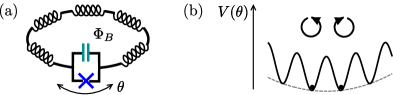
Figure 1: (a) Schematic picture of a fluxonium qubit. (b) Example of the potential for the phase difference across the single Josephson junction in a pure inductive loop and for external magnetic flux $\Phi_{B}=\Phi_{0}/2$. The two states associated with the local minima (black dots) correspond to the current eigenstates of the loop with supercurrents circulating in opposite directions (arrowed circles). Quantum phase tunnelling at the Josephson junction couples the two states.

For Josephson devices a particularly important achievement is the recent experimental realization of the fluxonium qubit [12, 13, 14, 21, 22] in which coherent quantum phase tunnelling is localized at a single weak junction of the Josephson chain. As shown in figure 1, in such a device a small junction is shunted with a series array of $N\gg 1$ identical large-capacitance Josephson tunnel junctions. The array of Josephson junctions acts as a superinductance which protects the small junction from offset charge variations. The junctions are characterized by a capacitance $C$, a maximal supercurrrent $I_{J}$, the Josephson energy $E_{J}=\hbar I_{J}/2e$, and the charging energy $E_{C}=e^{2}/2C$. Large phase fluctuations of order of $2\pi$ occur due to quantum tunnelling with an amplitude ${\cal V}$ which in the limit $E_{J}\gg E_{C}$ reads [6, 21, 25, 41]

$${\cal V}=4{(8E_{J}^{3}E_{C}/\pi^{2})}^{1/4}\exp(-\sqrt{8E_{J}/E_{C}}).$$ (1)

The fluxonium is realized for the condition

$$E_{J}/E_{C}\gg 1$$ (2)

for $N$ junctions so that large phase fluctuations of order of $2\pi$ are exponentially suppressed in the homogeneous part of the loop and each Josephson junction implements a linear inductance $L_{J}=\hbar^{2}/4e^{2}E_{J}$. In contrast, the weak element is characterized by the parameters $\bar{E}_{J}$ and $\bar{E}_{C}$ such that the amplitude of the phase tunnelling at the weak element is $\bar{{\cal V}}\gg{\cal V}$. More precisely, the relation

$$\bar{{\cal V}}\gg N{\cal V}$$ (3)

holds in the fluxonium which ensures that the inductive role of the junction array is not spoiled by large quantum phase fluctuations occurring in some part of it [1, 2, 6, 12, 25]. We note that the condition (3) still allows for exponentially long chains as long as $\bar{E}_{J}/\bar{E}_{C}\ll E_{J}/E_{C}$. Therefore, the non-linear excitations of the superconducting phase are strongly localized in one part of the superconducting ring. We remark that this is a special situation as, for instance, quantum phase slips in homogeneous superconducting nanowires and vortex excitations require a non-perturbative approach to treat the core of these non-linear excitations.

In this paper, we study coherent dynamics of the fluxonium device subject to an externally applied magnetic flux $\Phi_{B}$ as a function of the size of the system. We consider a one-dimensional ring composed of $N$ identical Josephson junctions and a weak element where the strong phase fluctuations of order of $2\pi$ take place. Such quantum phase fluctuations are localized exclusively at the weak element whereas the rest of the chain acts as an electromagnetic environment, provided the conditions (2) and (3) are satisfied. We focus on the two-level regime for a magnetic flux close to a half flux quantum $\Phi_{B}\approx\Phi_{0}/2$ ($\Phi_{0}=h/2e$) which is typical for experimental flux qubits devices. In this regime quantum tunnelling of the phase difference across the weak element coherently couples the two states with supercurrents circulating in the opposite directions. Taking into account the electrostatic interactions in the loop and in particular the capacitance to the ground, the homogeneous part of the loop different from the weak junction behaves as an ensemble of harmonic oscillators, similarly to electrodynamic modes of a transmission line of a finite length. We denote the spectrum of the modes by $\{\omega_{k}\}$, where $\omega_{1}$ is the lowest frequency which scales with the size of the system as $\omega_{1}\sim 1/N$.

We obtain the spectrum of electrodynamic modes $\{\omega_{k}\}$ in the ring and show that the local phase difference $\theta$ across the weak element couples to these modes which represent an effective (intrinsic) environment. We find that the frequencies $\omega_{k}$ are not equidistant and the modes’ coupling to the phase $\theta$ is non-uniform, with low-energy modes being more strongly coupled to $\theta$ than the high-energy ones. There are two qualitatively different dynamic regimes depending on the size of the system. For a small system, the frequency $\omega_{1}$ may be large such that the adiabatic condition $2\bar{\cal V}\ll\hbar\omega_{1}$ holds. In this case, the dynamics is given by that of a two-level system of the qubit, that is, it consists of quantum oscillations between the two counterpropagating supercurrent eigenstates. The effect of the high frequency modes is only the renormalization of the bare tunnelling amplitude, $\bar{{\cal V}}\to\tilde{{\cal V}}$. As the size of the system is increased, the frequencies of the modes decrease. The resonant condition $2\tilde{{\cal V}}=\hbar\omega_{1}$ is met for a certain number of junctions $N^{*}$ in series, where $2\tilde{{\cal V}}$ is the energy splitting between the first excited state and the ground state of the qubit. For $N>N^{*}$ the system enters the non-adiabatic regime in which some modes have frequencies smaller than the level splitting, $\hbar\omega_{k}<2\tilde{{\cal V}}$ for $k=1,\dots,n$. In this case, we find that the quantum dynamics is not periodic: it exhibits decay of oscillations at short times, followed by revival-like oscillations at longer times.

The remainder of the paper is organized as follows. In section 2, we recapitulate some of the results for the coherent phase tunnelling in the fluxonium qubit. Then, in order to facilitate a physical understanding of the effect of intrinsic electric modes on the quantum phase dynamics of the single junction, in section 3 we use a semi-analytical approach for a generic model of a particle in a double well potential coupled to a finite discrete bath of harmonic oscillators. We find that the dynamics of the particle has qualitatively different regimes (coherent and quasiperiodic) depending on the ratio between the tunnelling amplitude and the frequencies of the oscillators ($\hbar\omega_{1}\gg 2\tilde{{\cal V}}$ and $\hbar\omega_{1}\lesssim 2\tilde{{\cal V}}$). In section 4, we take into account the electrodynamics of the loop and map the fluxonium device to the model of section 3. We obtain the frequencies and the coupling strengths of electric modes of the ring and we analyze the experimental feasibility to observe the non-adiabatic dynamics. In section 5 we present our conclusions.

2 The model for the fluxonium

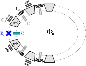
Figure 2: (colors online) Superconducting ring made of $N$ identical tunnelling junctions with inductance $L_{J}$ and capacitances $C$, and a weaker Josephson junction with Josephson energy $\bar{E}_{J}$ and capacitance $\bar{C}$. The ground capacitance of the superconducting islands between the junctions is $C_{0}$.

2.1 Single Josephson junction in an inductive loop

Let us consider a superconducting ring which consists of $N$ identical Josephson junctions and a weaker Josephson junction at which the strong phase fluctuations are localized, as has been discussed in the introduction. The system is shown in figure 2. If one neglects the electrostatic interactions in the homogeneous part of the loop, the array formed by $N$ identical Josephson junctions provides an inductance $L=NL_{J}$. This inductance sets the inductive energy $E_{L}=\hbar^{2}/4e^{2}L$. In this regime, the Hamiltonian of the system reads [12, 14, 21]

$$\hat{H}=4\bar{E}_{C}\hat{n}^{2}-\bar{E}_{J}\cos(\hat{\theta})+\frac{E_{L}}{2}{\left(\hat{\theta}-2\pi\frac{\Phi_{B}}{\Phi_{0}}\right)}^{2},$$ (4)

where $\hat{\theta}$ is the operator of the phase difference across the weak junction and $\hat{n}$ is its canonically conjugate operator ($[\hat{\theta},\hat{n}]=i$) that represents the number of Cooper pairs that have passed across the junction. Quasiparticle excitations and their dynamics can be disregarded at very low temperatures $k_{B}T\ll\Delta$, where $\Delta$ is the superconducting gap of the islands forming the Josephson ring. In general, non-equilibrium distribution and trapped quasiparticles can give rise to the decoherence of the flux qubit [21].

The spectrum of the Hamiltonian (4) was analyzed in [14]. The second and the third term in (4) represent the energy potential for the phase difference $\theta$. An example is shown in figure 1(b) for $\Phi_{B}=\Phi_{0}/2$ where the two absolute minima of the potential are degenerate and the two states are the eigenstates of the supercurrent circulating in the opposite directions in the loop. These states are distinguishable as they have different supercurrents. For large inductance $E_{L}\ll\bar{E}_{J}$, the two classical minima of the phase are given approximatively by $\pi E_{L}/\bar{E}_{J}$ and $2\pi(1-E_{L}/2\bar{E}_{J})$ with the associated supercurrents $\pm\Phi_{0}/4\pi L$. The first term in (4) is the electrostatic energy of the weak junction and it plays the role of inertial kinetic energy such that quantum tunnelling of the local phase difference $\theta$ can occur from one minimum to the nearest neighbor wells in the phase potential as shown in figure 1. The tunnelling amplitude can be obtained using semiclassical instanton or Wentzel-Kramers-Brillouin (WKB) method in the regime $\bar{E}_{C}\ll\bar{E}_{J}$. For $E_{L}\ll\bar{E}_{J}$, the profile of the energy barrier separating the two classical states is well approximated by the cosine potential and the tunnelling amplitude $\bar{{\cal V}}$ is still given by equation (1) with $E_{J}$ and $E_{C}$ replaced by $\bar{E}_{J}$ and $\bar{E}_{C}$ of the weak element. Corrections due to the parabolic part of the potential stemming from the loop inductance were discussed in [25].

For $E_{L}\gg 2\bar{{\cal V}}$, the quantum tunnelling effectively couples the two neighboring minima corresponding to the current eigenstates and the low-energy effective Hamiltonian can be described by a two-level model,

$$\hat{H}=E_{1}\left|1\right>\left<1\right|+E_{2}\left|2\right>\left<2\right|-\bar{{\cal V}}\left(\left|1\right>\left<2\right|+\left|2\right>\left<1\right|\right),$$ (5)

where $E_{i}=(E_{L}/2){(\theta_{i}-2\pi\Phi_{B}/\Phi_{0})}^{2}$ and $\theta_{i}$ are the positions of the two minima. Although we implicitly assumed $\Phi_{B}=\Phi_{0}/2$ for the derivation of the effective Hamiltonian (5), the obtained result is also applicable in a small range of fluxes centered around the half flux quantum for which the energy difference remains small as compared to the tunnelling amplitude, $|E_{1}-E_{2}|\ll\bar{{\cal V}}$. Thus, quantum tunnelling of the Josephson junction phase difference couples the counterpropagating supercurrent states, giving rise to the avoided crossing of the energy levels. The level splitting at the degeneracy point is $E_{S}=2\bar{{\cal V}}$. The splitting has been observed in fluxonium junctions close to degeneracy point [12, 22] and in superconducting nanowires [23, 24].

2.2 Single Josephson junction coupled to the electric modes of the loop

In this section we consider the superconducting Josephson ring taking into account the electrostatic interaction in the homogeneous part as shown in figure 2. Let $\phi_{n}$ be the superconducting phases of $N+1$ islands forming the ring. We denote the phase difference across the weak junction by $\theta=\phi_{0}-\phi_{N}$ whereas $\theta_{n}=\phi_{n+1}-\phi_{n}$ ($n=0,\dots,N-1$) are the phase differences across the Josephson junctions in the ring. The corresponding Euclidean Lagrangian (in the imaginary time $\tau$) of the system reads [25, 26, 42, 43, 44]

$${\mathscr{L}}=\sum_{n=0}^{N-1}\left[\frac{\hbar^{2}\dot{\theta}_{n}^{2}(\tau)}{16E_{C}}+\frac{\Phi_{0}^{2}}{2L_{J}}{\left(\frac{\theta_{n}(\tau)}{2\pi}+\frac{\Phi_{B}}{(N+1)\Phi_{0}}\right)}^{2}\right]+\sum_{n=0}^{N}\frac{\hbar^{2}\dot{\phi}_{n}^{2}(\tau)}{16E_{0}}+\bar{\mathscr{L}},$$ (6)

where the Euclidean Lagrangian of the weak element is

$$\bar{\mathscr{L}}=\frac{\hbar^{2}\dot{\theta}^{2}(\tau)}{16\bar{E}_{C}}-\bar{E}_{J}\cos\left(\theta(\tau)+\frac{2\pi\Phi_{B}}{(N+1)\Phi_{0}}\right).$$ (7)

Here, $\dot{\theta}=d\theta/d\tau$, $E_{C}=e^{2}/2C$ and $E_{0}=e^{2}/2C_{0}$ are the charging energies of the islands with $C$ being the junction capacitance and $C_{0}$ the capacitance of the islands to the ground. The weak junction is characterized by $\bar{E}_{J},\bar{E}_{C}$ where $\bar{E}_{J}<E_{J}$ and $\bar{E}_{C}>E_{C}$. The phases $\theta_{n}+2\pi(\Phi_{B}/\Phi_{0})/(N+1)$ in (6) and (7) are the gauge invariant phase differences across the junctions. Due to the phase periodicity $\phi_{n}=\phi_{n+N+1}+2\pi m$ ($m$ integer), the variable $\theta$ and the set of $N$ phase differences $\{\theta_{n}\}$ satisfy the constraint

$$\theta(\tau)+\sum_{n=0}^{N-1}\theta_{n}(\tau)=0\quad\left(\rm{mod\ }2\pi\right).$$ (8)

Using the path-integral formalism, one can write the partition function of the system as

$${\cal Z}=\oint{\cal D}\theta\prod_{n=0}^{N-1}\oint{\cal D}\theta_{n}\exp\left(-\frac{1}{\hbar}\int^{\beta}_{0}d\tau{\mathscr{L}}\right)$$ (9)

where $\beta=\hbar/(k_{B}T)$.

Before concluding this section, we note that equation (4) can be simply recovered from (6) and (7) by neglecting the electrostatic interaction for the $N$ junctions in the chain and using the constraint (8) for the phase difference to impose $\theta_{n}=\theta/N$ in the limit $N\gg 1$.

3 Effective model

Before we proceed with the study of dynamics of the quantum phase tunnelling across the weak element coupled to electric modes of the loop, in this section we first analyze a generic model of a particle in a double-well potential interacting with a discrete bosonic bath. Mapping of the Josephson junction chain to this model is given in section 4.

Let us consider a particle moving in a double-well potential and interacting with a bosonic bath of $N$ harmonic oscillators, see figure 3. If the height of the barrier is larger than the kinetic energy $E\sim\hbar^{2}/ma_{0}^{2}$, the system can be reduced to the states $|R\rangle$ and $|L\rangle$ localized at the positions $x=\pm a_{0}$ which are coupled by quantum tunnelling. This is a well-known spin-boson model[45, 46, 47] with the Hamiltonian

$$\hat{H}=\bar{\cal V}\,\hat{\sigma}_{x}+\hat{\sigma}_{z}\sum_{k=1}^{N}\alpha_{k}\hbar\omega_{k}\left(\hat{a}_{k}^{\dagger}+\hat{a}_{k}\right)+\sum_{k=1}^{N}\hbar\omega_{k}\hat{a}_{k}^{\dagger}\hat{a}_{k}.$$ (10)

Here, $\hat{\sigma}_{x}=|L\rangle\langle R|+|R\rangle\langle L|$, $\hat{\sigma}_{z}=|L\rangle\langle L|-|R\rangle\langle R|$, $\hat{a}_{k}^{\dagger}$ ($\hat{a}_{k}$) are creation (annihilation) operators of the oscillator modes $\omega_{k}$, $\alpha_{k}$ are the coupling constants, and $\bar{\cal V}$ is the bare tunnelling amplitude between the states $|L\rangle$ and $|R\rangle$.

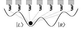
Figure 3: Particle in a double-well potential coupled to $N$ harmonic oscillators. States localized around the two potential minima are denoted by $|L\rangle$ and $|R\rangle$, respectively.

The two energy-degenerate states correspond to the counterpropagating supercurrent states at half flux quantum as discussed in section 2, whereas the harmonic oscillators represent electric modes of the homogeneous part of the superconducting loop in which large phase fluctuations are suppressed as discussed in section 1. The coupling constants are related to the characteristic impedance of the homogeneous part of the loop, see section 4.

For a large number of oscillators and linear low-frequency dispersion ($N\to\infty$, $\delta\omega\to 0$, $\omega_{k}=k\delta\omega$) one recovers the standard Caldeira-Leggett model[48] which describes the dissipative quantum dynamics of the two-level system coupled to an ohmic environment. This system has been studied extensively in the literature [48, 45, 46, 47]. Here we just recall that the high-energy modes with $\hbar\omega_{l}\gg 2\bar{\cal V}$ quickly adjust themselves to the slow tunnelling motion of the particle and hence can be treated adiabatically. These modes give rise to a renormalization of the tunnelling amplitude,

$$\tilde{\cal V}=\bar{\cal V}\,e^{-\sum_{l}\alpha_{l}^{2}/2}.$$ (11)

3.1 Non-adiabatic dynamics

In contrast to the usual dissipative case, in what follows we focus on a bath with discrete low-energy spectrum $\omega_{k}=k\delta\omega$, where the level spacing $\delta\omega$ is fixed. The adiabatic renormalization of the tunnelling amplitude by high-frequency modes in (11) does not depend on the type of the bosonic bath: it is valid for a single oscillator, a discrete set of oscillators, or a continuum dense distribution [49]. On the other hand, the low frequency modes that are smaller or comparable to the tunnelling amplitude are responsible for a non-adiabatic dynamics of the particle. Depending on the density of the low-frequency modes, the dynamics can be quasiperiodic for a few discrete modes or dissipative for a dense continuum of modes.

Let us first separate bath eigenmodes into the low-energy ($\omega_{k}<\omega_{c}$) and the high-energy ($\omega_{k}>\omega_{c}$) ones. The high-energy modes renormalize the bare tunnelling amplitude according to (11), while the low-energy modes determine the details of the particle dynamics. The choice of the cutoff frequency $\omega_{c}$ is nonessential provided it is much larger than the frequency of particle tunnelling, $\omega_{c}\gg 2\tilde{\cal V}/\hbar$ (see figure 4 and Appendices A and B). In this case, the system is described by the Hamiltonian (10) with $\bar{\cal V}$ replaced by $\tilde{\cal V}$ and $N$ replaced by $N_{c}$, where $\omega_{k}$ ($k=1,\ldots,N_{c}$) are the low-energy modes.

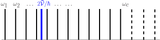
Figure 4: (colors online) Bath energy spectrum in the non-adiabatic regime where several discrete modes have frequencies smaller or comparable to the tunnelling frequency $2\tilde{\cal V}/\hbar$.

Next, we apply a polaron unitary transformation $\hat{H}^{\prime}=e^{\hat{\sigma}_{z}\hat{D}}\hat{H}e^{-\hat{\sigma}_{z}\hat{D}}$ with $\hat{D}=\sum_{k=1}^{N_{c}}\alpha_{k}\left(\hat{a}_{k}^{\phantom{g}}-\hat{a}_{k}^{\dagger}\right)$, in which the oscillators are displaced depending on the state of a particle. The transformed Hamiltonian reads

$$\hat{H}^{\prime}=\tilde{\cal V}\,\left(\hat{\sigma}_{-}e^{-\hat{D}}+\hat{\sigma}_{+}e^{\hat{D}}\right)+\sum_{k=1}^{N_{c}}\hbar\omega_{k}^{\phantom{g}}\hat{a}_{k}^{\dagger}\hat{a}_{k}^{\phantom{g}},$$ (12)

where $\hat{\sigma}_{-}=|L\rangle\langle R|$, $\hat{\sigma}_{+}=|R\rangle\langle L|$, and we omitted an unimportant additive constant in $\hat{H}^{\prime}$. For zero coupling $\hat{D}=0$ the tunneling of the free particle is recovered ($\hat{\sigma}_{-}+\hat{\sigma}_{+}=\hat{\sigma}_{x}$). The time evolution of $\hat{\sigma}_{\pm}$ with respect to $H^{\prime}$ is given by

$$\hat{\sigma}_{\pm}(t)=\hat{\sigma}_{\pm}(0)\pm\frac{i2\tilde{\cal V}}{\hbar}\int_{0}^{t}dt^{\prime}\,e^{\mp\hat{D}(t^{\prime})}\hat{\sigma}_{z}(t^{\prime}).$$ (13)

Substituting $\hat{\sigma}_{\pm}(t)$ in the equation of motion for $\sigma(t)\equiv\langle\hat{\sigma}_{z}(t)\rangle$, we obtain

$$\frac{d\sigma(t)}{dt}=\frac{i\tilde{\cal V}}{\hbar}\left\langle e^{\hat{D}(t)}\hat{\sigma}_{+}(t)-\hat{\sigma}_{-}(t)e^{-\hat{D}(t)}\right\rangle=-\frac{4\tilde{\cal V}^{2}}{\hbar^{2}}\int_{0}^{t}dt^{\prime}\,{G}(t-t^{\prime})\,\sigma(t^{\prime}),$$ (14)

where

$${G}(t-t^{\prime})\equiv\text{Re}\,\left\langle e^{\hat{D}(t)}e^{-\hat{D}(t^{\prime})}\right\rangle=\text{Re}\,\left(e^{J(t-t^{\prime})}\right)$$ (15)

with $J(t)=-\sum_{k=1}^{N_{c}}\alpha_{k}^{2}(1-e^{-i\omega_{k}t})$. Here we have used the initial condition $\langle\hat{\sigma}_{\pm}(0)\rangle=0$ and the noninteracting blip approximation (NIBA)[45, 46, 50, 51, 52] to factorize the average of a product of particle and bath operators. The approximation is based on the assumption that the dynamics of the bath is weakly perturbed by the particle ($\alpha_{k}^{2}\ll 1$), whereas the back-action of the bath on the particle is taken into account ($\sum_{k}\alpha_{k}^{2}\sim N\alpha_{k}^{2}$).

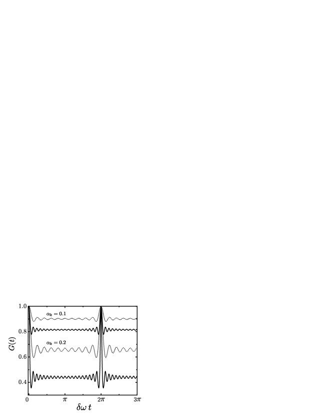
Figure 5: The kernel ${G}(t)$ for the bath with $N_{c}=10$ modes (dotted) and $N_{c}=20$ modes (solid curve) and the coupling strength $\alpha_{k}=0.1$ (top) and $\alpha_{k}=0.2$ (bottom). The frequencies of the modes are assumed equidistant, $\omega_{k}=k\delta\omega$.

For a state $|\psi(t)\rangle=c_{L}(t)|L\rangle+c_{R}(t)|R\rangle$, the quantity $\sigma(t)=|c_{L}(t)|^{2}-|c_{R}(t)|^{2}$ measures the degree of superposition of $|L\rangle$ and $|R\rangle$ states. Equation (14) describes the particle dynamics in a closed form for a given kernel ${G}(t-t^{\prime})$ characterizing the bath. The kernel ${G}(t)$ is shown in figure 5 for equidistant bath frequencies $\omega_{k}=k\delta\omega$ and different number of modes $N_{c}$ and the coupling strengths $\alpha_{k}$. At a given coupling constant $\alpha_{k}$, for $N_{c}\sim 1$, the kernel ${G}(t)$ exhibits oscillations with a small amplitude and period $\tau_{r}=2\pi/\delta\omega$ which corresponds to the revival time. When the number of modes $N_{c}$ is increased, the kernel ${G}(t)$ decays at short times with a time constant $(\sum_{k}\alpha_{k}^{2}\omega_{k}^{2}/2)^{-1/2}$ which corresponds to the typical duration of the revivals occurring after a period $\tau_{r}$. To complete the analysis, we note that ${G}(t)$ has also another time scale $\tau_{s}$ for high cut-off $N_{c}$, associated with the fast oscillations inside the duration of one revival, with frequency $\sim\sum_{k}\alpha_{k}^{2}\omega_{k}$.

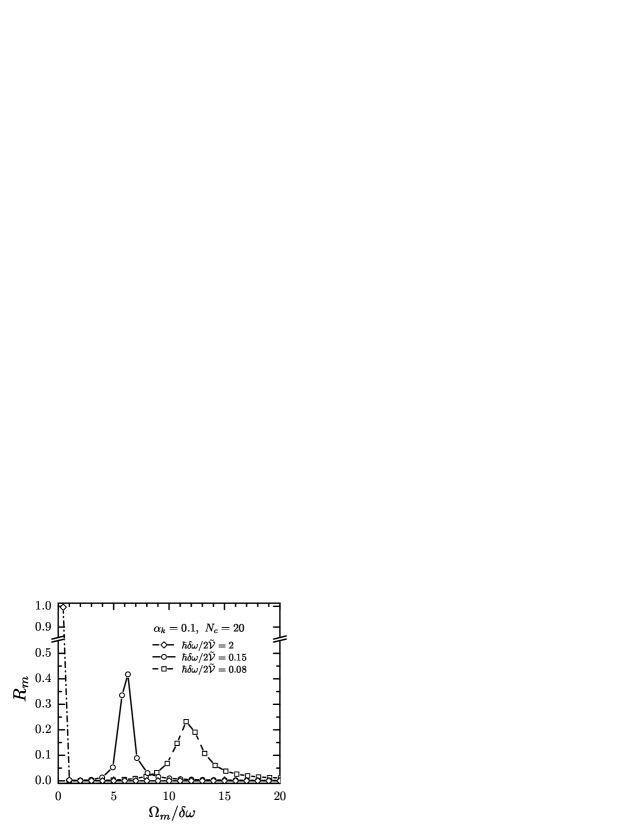
Figure 6: Frequency spectrum for a particle coupled to a bath of $N_{c}=20$ modes with $\alpha_{k}=0.1$ and the level spacing $\hbar\delta\omega/2\tilde{\cal V}=2$ (diamonds), $0.15$ (circles), and $0.08$ (squares).

In what follows we solve (14) assuming equidistant low-energy spectrum of the bath $\omega_{k}=k\delta\omega$ ($k=1,\ldots,N_{c}$). Taking the Laplace transform of (14) we obtain

$$\sigma(s)=\frac{\sigma_{0}}{s+(4\tilde{\cal V}^{2}/\hbar^{2}){G}(s)}$$ (16)

where $\sigma_{0}\equiv\sigma(t=0)$ and ${G}(s)=\sum_{m=0}^{\infty}c_{m}s/(s^{2}+\omega_{m}^{2})$. The coefficients $c_{m}$ are given by

$$c_{m}=e^{-\sum_{k}\alpha_{k}^{2}}\sideset{}{{}^{\prime}}{\sum}_{\{k\}}\frac{\alpha_{1}^{2k_{1}}\alpha_{2}^{2k_{2}}\cdots\alpha_{N_{c}}^{2k_{N_{c}}}}{k_{1}!k_{2}!\cdots k_{N_{c}}!}$$ (17)

where ^′ denotes summation over $k_{n}\geq 0$ with constraint $\sum_{n=1}^{N_{c}}nk_{n}=m$. The constraint takes into account the degeneracy of the energy eigenstate $\hbar\omega_{m}$ of the bath. Coefficients $c_{m}$ obey the sum rule $\sum_{m=0}^{\infty}c_{m}=1$. We recall that the coupling of the particle to the bath is assumed to be small, $\alpha_{k}^{2}\ll 1$, but may vary as a function of $k$ for different modes $\omega_{k}$ of the bath.

Equation (16) has poles at $s=\pm i\Omega_{m}$, where $\omega_{m}<\Omega_{m}<\omega_{m+1}$ ($m=0,1,\ldots$). Taking the inverse Laplace transform of (16) we obtain

$$\sigma(t)=\sigma_{0}\sum_{m=0}^{\infty}R_{m}\cos(\Omega_{m}t)$$ (18)

with $R_{m}=\prod_{n=1}^{\infty}(\omega_{n}^{2}-\Omega_{m}^{2})/\prod^{\prime}\!{}_{n=0}^{\infty}(\Omega_{n}^{2}-\Omega_{m}^{2})$. Here, ^′ denotes that the term with $n=m$ is omitted in the denominator of $R_{m}$.

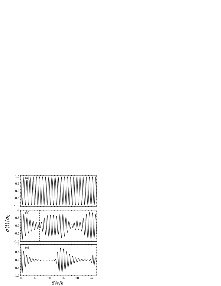
Figure 7: Average position $\sigma(t)$ for a particle coupled to a discrete bath with $N_{c}=20$, $\alpha_{k}=0.1$, and the level spacing (a) $\hbar\delta\omega/2\tilde{\cal V}=2$, (b) $\hbar\delta\omega/2\tilde{\cal V}=0.15$, and (c) $\hbar\delta\omega/2\tilde{\cal V}=0.08$. The corresponding frequency spectra are shown in figure 6. Dashed lines in (b) and (c) indicate the onset of revivals at $t=2\pi/\delta\omega$.

A crossover from adiabatic to non-adiabatic dynamics is shown in figures 6 and 7 for a particle coupled to a bath with $N_{c}=20$ modes, $\alpha_{k}=0.1$, and the level spacing $\hbar\delta\omega/2\tilde{\cal V}=2$, $0.15$, and $0.08$, respectively. The average position of a particle $\sigma(t)$ is shown in figure 7. In the adiabatic case $\hbar\delta\omega/2\tilde{\cal V}=2$, we observe in figure 6 that only the lowest frequency is relevant. It is approximately equal to the renormalized frequency given by (11) with the sum including all the modes (see A). In this case the dynamics corresponds simply to coherent oscillations shown in figure 7(a). As the density of the modes is increased, several frequencies $\Omega_{m}$ start to contribute, with amplitudes $R_{m}$ shown in figure 6. In the weak coupling regime which we consider, the particle still oscillates between the two minima with the frequency $2\tilde{\cal V}/\hbar$ corresponding to the fast oscillations in figures 7(b) and (c). The amplitude of these oscillations initially decays as the bath modes are populated and the energy is transferred from the particle to the bath. The decay time is $\tau_{d}\propto\hbar^{2}/\tilde{\cal V}^{2}\sqrt{(\sum_{k}\alpha_{k}^{2}\omega_{k}^{2})/(\sum_{k}\alpha_{k}^{2})}$. However, after time $\tau_{r}=2\pi/\delta\omega$, the populated bath modes start to feed energy back to the particle and revivals of oscillations take place. From that point on, we have two different behaviors depending on the ratio $\tau_{d}/\tau_{r}$. For $\tau_{d}\lesssim\tau_{r}$, the dynamics of a particle has a form of a quasiperiodic beating instead of a decay. Reducing $\tau_{d}\ll\tau_{r}$, the dynamics exhibits again a decay after a revival of the oscillation amplitude. For a dense continuum of bath modes ($N_{c}\to\infty$, $\delta\omega\to 0$) the revival time is infinite, $\tau_{r}\to\infty$. In this case the bath cannot feed significant amounts of energy back to the particle and one recovers exponentially damped oscillations characteristic for Ohmic dissipation.

4 Josephson junction ring with a weak element

Here we show how the dynamics of the quantum tunnelling between the two counterpropagating supercurrent states discussed in section 2 can be mapped to the spin-boson model of section 3 when the electric modes of the ring are taken into account.

First we cast (6) and (7) in the form in which the coupling of $\theta$ to electric modes of the ring is manifest [25]. We take as independent variables the phases between Josephson junctions, $\varphi_{n}\equiv\phi_{n}$ for $n=1,\dots,N-1$, the average phase $\varphi_{0}\equiv(\phi_{0}+\phi_{N})/2$ and the phase difference $\theta$ across the weak element. Since $\varphi_{n}$ is periodic on the effective lattice $n=0,\dots,N-1$ composed of $N$ elements, it can be Fourier transformed as $\varphi_{n}=(1/\sqrt{N})\sum^{N-1}_{k=0}\varphi_{k}\exp(i2\pi nk/N)$ where $\varphi_{N-k}=\varphi_{k}^{*}$. The real and imaginary parts $\varphi^{\prime}_{k}$ and $\varphi^{\prime\prime}_{k}$ of $\varphi_{k}$ give rise to even and odd modes, respectively. After the substitution in (6) and (7), we find that only $\varphi^{\prime\prime}_{k}$ couple to $\theta$ while $\varphi^{\prime}_{k}$ describe a set of decoupled harmonic oscillators. Since $\varphi^{\prime\prime}_{N-k}=-\varphi^{\prime\prime}_{k}$, only half of the modes are independent; we label these modes with $k$, $1\leq k\leq k_{\rm max}$, where $k_{\rm max}=\lfloor(N-1)/2\rfloor$ and $\lfloor x\rfloor$ is the integer part of $x$. The Euclidean Lagrangian in the imaginary time reads ${\mathscr{L}}={\mathscr{L}}_{0}+{\mathscr{L}}_{\rm int}$ where

$${\mathscr{L}}_{0}=\frac{\hbar^{2}\dot{\theta}^{2}}{16E_{\tilde{C}}}-\bar{E}_{J}\cos(\theta+\delta_{B})+\frac{E_{L}}{2}(\theta-N\delta_{B})^{2}$$ (19)

and

$${\mathscr{L}}_{\rm int}=\sum_{k=1}^{k_{\rm max}}\left\{\frac{\mu_{k}}{2}\dot{X}_{k}^{2}+\frac{\mu_{k}\omega_{k}^{2}}{2}\left[X_{k}-\left(\frac{\omega_{p}^{2}}{\omega_{k}^{2}}-1\right)\frac{f_{k}}{\mu_{k}}\theta\right]^{2}\right\},$$ (20)

with $\delta_{B}=2\pi(\Phi_{B}/\Phi_{0})/(N+1)$ and $X_{k}=\varphi^{\prime\prime}_{k}-(f_{k}/\mu_{k})\theta$. Here, $\mu_{k}=(8E_{J}/\omega_{k}^{2})\sin^{2}(\pi k/N)$, $f_{k}=(2E_{J}/\sqrt{N}\omega_{p}^{2})\sin(2\pi k/N)$, and $\omega_{p}=1/\sqrt{L_{J}C}$.

The Lagrangian ${\mathscr{L}}_{0}$ describes the phase $\theta$ in a double-well potential with two degenerate minima at half flux quantum ($L\gg\bar{L}_{J}$, where $L=NL_{J}$ is the effective inductance of the ring; $\bar{L}_{J}$ is inductance of the weak junction). The minima correspond to the counterpropagating supercurrent states that enter the spin-boson model and which are coupled by the quantum phase tunnelling, cf. section 3 and figure 3 [1, 6, 25]. Josephson junctions in the chain give rise to a renormalization of the charging energy of the weak element $E_{\tilde{C}}=e^{2}/2\tilde{C}$, where

$$\tilde{C}=\bar{C}+\frac{C}{N}+\frac{C_{0}}{2}\left(1+\frac{1}{N}\sum_{k=1}^{k_{\rm max}}\frac{\cos^{2}(\pi k/N)}{\sin^{2}(\pi k/N)+C_{0}/4C}\right).$$ (21)

By taking the thermodynamic limit $N\rightarrow\infty$ in (21), we recover the renormalization of the capacitance of the weak junction as obtained in [43] (see further discussions in [25]). On the other hand, when the capacitance to the ground is small, $N\sqrt{C_{0}/C}\ll 1$, we obtain $\tilde{C}=\bar{C}+C/N+C_{0}/2+C_{0}(N-1)(N-2)/12N$ which is in agreement with [53]. This result can be obtained by setting $C_{0}=0$ in the sum over $k$ in (21).

The Lagrangian ${\mathscr{L}}_{\rm int}$ in (20) contains the harmonic modes in the ring whose dispersion relation reads[25]

$$\omega_{k}=\frac{\omega_{p}\sin(\pi k/N)}{\sqrt{\sin^{2}(\pi k/N)+C_{0}/4C}}.$$ (22)

Note that the potential term in (20) does not confine $\theta$ because it depends on the relative coordinates with respect to the bath degrees of freedom. Moreover, we note that the ground capacitance plays a crucial role: For $C_{0}=0$ the dispersion relation becomes flat with $\omega_{k}=\omega_{p}$ and the weak junction is decoupled from the electric modes of the ring, see (20). In that case, the only effect of the Josephson ring is the presence of the adiabatic confining potential in ${\mathscr{L}}_{0}$ associated with the ring’s inductance. This result is in agreement with previous works [6, 25, 53] in which it was shown that the modes of the Josephson chains are decoupled from the weak element in the harmonic approximation and for $C_{0}=0$.

The harmonic modes of the ring can be integrated out using the Feynman-Vernon influence functional in the real-time path integral approach. For the model (10), the resulting influence action which governs the dynamics of the two levels is a functional of the spectral density of the modes

$$F(\omega)=\frac{\hbar}{\pi}\sum_{k}\alpha_{k}^{2}\omega_{k}^{2}\delta(\omega-\omega_{k}).$$ (23)

In a similar way, the linear coupling of the phase difference $\theta$ at the weak element to an ensemble of harmonic oscillators affects the dynamics of $\theta$ only through $F(\omega)$, regardless of the details of the bath [46, 45]. Hence, from the knowledge of the coupling constants $\alpha_{k}$ and the spectrum $\omega_{k}$ one can analyze the real-time dynamics of the quantum tunnelling between the two low-energy states in a double-well potential of equation (19) using the effective spin-boson model as described in section 3.

Instead of carrying out a calculation in the real-time formalism, we can proceed with the imaginary-time one and make use of a relation[46]

$$K_{l}=\frac{2}{\pi}\int^{\infty}_{0}\!\!\!\!d\omega\frac{\nu_{l}^{2}F(\omega)}{\omega(\nu_{l}^{2}+\omega^{2})}=\frac{2\hbar}{\pi^{2}}\sum_{k}\alpha_{k}^{2}\frac{\nu_{l}^{2}\omega_{k}}{\nu_{l}^{2}+\omega_{k}^{2}}$$ (24)

between $F(\omega)$ and the kernel $K_{l}=K(\nu_{l})$ of the imaginary-time effective action ($\nu_{l}=2\pi l/\beta$ are the Matsubara frequencies). Kernel $K_{l}$ can be obtained from the partition function of the system which is given by imaginary-time path integral over closed trajectories $\theta(0)=\theta(\beta)$ and $X_{k}(0)=X_{k}(\beta)$:

$${\cal Z}_{\rm tot}=\oint{\cal D}\theta{\cal D}X\,e^{-(S_{0}+S_{\rm int})/\hbar},$$ (25)

where $S_{0}[\theta]=\int_{0}^{\beta}d\tau{\mathscr{L}}_{0}[\theta]$ and $S_{\rm int}[\theta,X]=\int_{0}^{\beta}d\tau{\mathscr{L}}_{\rm int}[\theta,X]$. After integrating out bath degrees of freedom, one obtains ${\cal Z}_{\rm tot}={\cal Z}_{h}\times{\cal Z}$, where ${\cal Z}_{h}=\prod_{k}[2\sinh(\beta\omega_{k}/2)]^{-1}$ is the partition function of harmonic oscillators and

$${\cal Z}=\oint{\cal D}\theta\,e^{-(S_{0}+S_{\rm inf})/\hbar}$$ (26)

is the partition function of the particle interacting with the bath. The interaction is included in the influence action

$$S_{\rm inf}[\theta]=\frac{1}{2}\int_{0}^{\beta}\!\!\!\!\!d\tau d\tau^{\prime}\theta(\tau)K(\tau-\tau^{\prime})\theta(\tau^{\prime})=\frac{1}{\beta}\sum_{l=1}^{\infty}K_{l}|\theta_{l}|^{2},$$ (27)

where $\theta_{l}=\int_{0}^{\beta}d\tau\,\theta(\tau)e^{i\nu_{l}\tau}$. After integration of the harmonic modes in ${\mathscr{L}}_{\rm int}$, we obtain

$$S_{\rm inf}[\theta]=\frac{1}{\beta}\sum_{l=1}^{\infty}|\theta_{l}|^{2}\sum_{k=1}^{k_{\rm max}}\frac{\nu_{l}^{2}}{\nu_{l}^{2}+\omega_{k}^{2}}\left(\frac{f_{k}^{2}\omega_{p}^{4}}{\mu_{k}\omega_{k}^{2}}\right)\left(1-\frac{\omega_{k}^{2}}{\omega_{p}^{2}}\right)^{2},$$ (28)

and using (24) and (27) we extract the coupling constants:

$$\alpha_{k}=\frac{\pi}{\sqrt{N}}\left(\frac{E_{J}}{\hbar\omega_{k}}\right)^{\!1/2}\!\!\left(1-\frac{\omega_{k}^{2}}{\omega_{p}^{2}}\right)\cos(\pi k/N).$$ (29)

Equations (22) and (29) for the frequencies $\omega_{k}$ of electric modes in the loop and the coupling constants $\alpha_{k}$, respectively, complete the mapping of the Josephson junction ring with a weak element to a generic spin-boson model of section 3.

For a non-zero capacitance to the ground and large number of junctions in the ring, $N\sqrt{C_{0}/C}\gg 1$, the dispersion at low frequencies is linear, $\omega_{k}\approx(2\pi k/N)\omega_{0}$ ($\omega_{0}=1/\sqrt{L_{J}C_{0}}$). In this case, the coupling constants at low frequencies are given by

$$\alpha_{k}=\frac{1}{2}\sqrt{\frac{R_{q}}{Z_{0}}}\frac{1}{\sqrt{k}}\qquad(k<N_{c}),$$ (30)

where $R_{q}=h/4e^{2}$ is the quantum resistance and $Z_{0}=\sqrt{L_{J}/C_{0}}$ is the low-frequency transmission-line impedance of the ring. The cutoff frequency $\omega_{c}=\omega_{k=N_{c}}$ with $\sin(\pi N_{c}/N)=\sqrt{C_{0}/4C}$ discriminates between a linear (low-frequency) and a nonlinear (high-frequency) part of the spectrum. As long as $2\tilde{{\cal V}}<\hbar\omega_{p}$, this frequency also divides the low-frequency modes responsible for the details of the phase dynamics from the high-frequency modes which only renormalize the phase slip amplitude.

Before we conclude this section, let us also consider the case of the small capacitance to the ground, $N\sqrt{C_{0}/C}\ll 1$. The coupling constants in this case are given by $\alpha_{k}\approx(1/4\pi)(C_{0}/C)(E_{J}/8E_{C})^{1/4}N^{3/2}/k^{2}$. The effective Hamiltonian of the weak junction coupled to the electric modes of the ring is given by $\hat{H}_{eff}=-4E_{\tilde{C}}\partial_{\hat{\theta}}^{2}+V(\hat{\theta})+(\hat{\theta}/\pi)\sum_{k}\alpha_{k}\hbar\omega_{k}(\hat{a}_{k}^{\dagger}+\hat{a}_{k})+\sum_{k}\hbar\omega_{k}\hat{a}_{k}^{\dagger}\hat{a}_{k}.$ By applying the unitary transformation $\hat{U}^{\dagger}\hat{H}_{eff}\hat{U}$ where $\hat{U}=\exp[(\hat{\theta}/\pi)\sum_{k}\alpha_{k}(\hat{a}_{k}-\hat{a}_{k}^{\dagger})]$ we can cast the Hamiltonian in the form in which the coupling is expressed in terms of momenta rather than coordinates. We obtain $\hat{U}^{\dagger}\hat{H}_{eff}\hat{U}=-4E_{\tilde{C}}\partial_{\hat{\theta}}^{2}+V(\hat{\theta})-\sum_{k}\lambda_{k}(\hat{a}_{k}-\hat{a}_{k}^{\dagger})\partial_{\hat{\theta}}+\sum_{k}\hbar\omega_{k}\hat{a}_{k}^{\dagger}\hat{a}_{k}$, with $\lambda_{k}=(8/\pi^{2})E_{\tilde{C}}(C_{0}/C)(E_{J}/8E_{C})^{1/4}N^{3/2}/(2k)^{2}$. The obtained coupling term $-\sum_{k}\lambda_{k}(\hat{a}_{k}-\hat{a}_{k}^{\dagger})\partial_{\hat{\theta}}$ between the weak element and the modes of the ring is in agreement with the results of Ferguson et al. [53].

4.1 Discussion of the experimental observability

In the following we analyze the feasibility of achieving a non-adiabatic dynamics in realistic superconducting rings made of Josephson junctions. Since the capacitance of the junction is proportional to the cross section area while inductance is inversely proportional to it, we have $L_{J}C=\bar{L}_{J}\bar{C}$. In this case, the condition $NL_{J}\gg\bar{L}_{J}$ for the system to be in a well-defined flux state implies $\bar{C}\gg C/N$ and the renormalization of the capacitance of the weak element in (21) is negligible. The hierarchy of energy scales $N{\cal V}\ll\tilde{\cal V}\ll E_{L}$ discussed in section 2 gives the upper limit of the ring length, $N\ll N_{a},N_{b}$, where $N_{a}=\sqrt{L_{J}/\bar{L}_{J}}\exp[(4/\pi)R_{q}(Z_{J}^{-1}-\bar{Z}_{J}^{-1})]$ and $N_{b}\approx 3.5(\bar{L}_{J}/L_{J})\sqrt{R_{q}/\bar{Z}_{J}}\exp[(4/\pi)R_{q}/\bar{Z}_{J}]$ with $Z_{J}=\sqrt{L_{J}/C}$ and $\bar{Z}_{J}=\sqrt{\bar{L}_{J}/\bar{C}}$. These conditions are not very restrictive and can be met in realistic devices, as demonstrated experimentally in the fluxonium superconducting chain with $N=43$ Josephson junctions in series [12]. In addition to the previous conditions, for non-adiabatic phase dynamics to occur the lowest frequency of electric modes has to be smaller than the qubit level splitting, $\hbar\delta\omega=2\pi\hbar\omega_{0}/N<2\tilde{\cal V}$. This can be achieved, e.g., by making the ground capacitance larger than a certain threshold, $C_{0}>(\pi\hbar/N\tilde{\cal V})^{2}L_{J}^{-1}$.

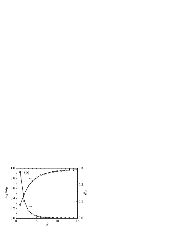
Figure 8: (a) Non-adiabatic dynamics of a flux qubit made of a Josephson junction chain with a weak element. Parameters are $\bar{C}/C=0.1$, $C_{0}/C=0.05$, $Z_{J}/R_{q}=0.18$, $N=100$, and $\hbar\omega_{p}/\tilde{\cal V}=3$. (b) Dispersion $\omega_{k}$ (circles, left axis) and the coupling constants $\alpha_{k}^{2}$ (squares, right axis) of the modes in the chain.

As an example, we take $N=100$ junctions in series, $\bar{C}/C=0.1$, $C_{0}/C=0.05$, and $Z_{J}/R_{q}=0.18$. The dispersion of the modes and the coupling constants are given by (22) and (29), respectively, see figure 8(b). The non-adiabatic dynamics of the qubit is shown in figure 8(a) obtained by numerical solution of (14). At half flux quantum, the neighboring phase-slip states carry the counterpropagating persistent currents of the same magnitude and $\sigma(t)$ is proportional to the average current through the loop, $\sigma(t)\propto I(t)$. The dynamics exhibits the same qualitative features (initial decay and revivals) as discussed in section 3 for a generic model with equidistant spectrum of the modes and constant coupling of the phase to the bath degrees of freedom. When the number of junctions or the strength of the coupling $\alpha_{k}$ is increased (e.g., by increasing the capacitance $C_{0}$ to the ground), the number of electric modes that are coupled to the phase increases and the transition to coherent non-adiabatic dynamics takes place. Recent experiments reported the fabrication of long Josephson junction chains comparable in order of magnitude to our example and operating as linear “superinductance” elements in which quantum phase slips are suppressed [44]. Dispersion of the modes in this system has also been measured. In addition, Josephson junction chains in the ladder geometry have been studied experimentally [54]. In this system, quantum phase tunnelling is prevented at the topological level which opens the route towards realization of long Josephson junction chains behaving as perfect inductances.

The condition for the observation of the quasiperiodic dynamics is that the relaxation and dephasing times of a qubit are larger than the revival period $\tau_{r}$. Estimating $\tau_{r}\sim 2\pi/\delta\omega$ with $\delta\omega=0.01\omega_{p}$ and $\omega_{p}\sim 1$GHz, we obtain $\tau_{r}$ of order of $\mu$s. This is well below the measured relaxation and dephasing times which can approach hundreds and tens of $\mu$s, respectively, in the present devices [55, 56]. Moreover, the experimental resolution for monitoring the qubit which has been achieved so far can be around of hundred of nanoseconds pointing out that the observation of the quasiperiodic dynamics is within the reach of the present technology.

5 Conclusion

In conclusion, we have studied quantum dynamics between two macroscopic supercurrent states in superconducting one-dimensional rings with a weak element and threaded by a magnetic flux. For sufficiently large system size, we have found that the quantum dynamics can be more complex than the usual coherent oscillations between the two states characterized by the quantum phase tunnelling amplitude. Such a dynamics emerges due to the coupling between the phase difference at the weak element and the intrinsic electrodynamic modes in the homogeneous part of the ring. We have obtained the spectrum of the modes in the ring and the corresponding coupling constants and have shown that in the non-adiabatic regime the dynamics of the system is quasiperiodic with exponential decay of oscillations at short times followed by oscillation revivals at later times. Revivals can be observed in a typical flux qubit setup in which the state of the qubit is measured. We have discussed the experimental feasibility to observe the quasiperiodic dynamics and revivals in realistic systems with large number of Josephson junctions in series or in systems with a finite charging energy of the islands between the junctions due to a non-zero capacitance to the ground.

Recent experiments have shown that a larger number of degrees of freedom is not necessarily penalized by decoherence [22, 57, 53, 58, 56, 55], thus opening the possibility to explore novel dynamic regimes beyond the two-level’s one. Observation of a quasiperiodic dynamics would be important for understanding the mechanisms of decoherence in large quantum circuits as well as intrinsic limits on coherence posed by the circuit itself. Our results can also be of interest for the design of models with a tunable fictitious dissipation or, for instance, to achieve controlled quantum evolution in superconducting qubits by engineering the parameters of the Josephson junction circuits. This motivates future studies of flux qubits realized in large superconducting circuits with a more complex topological structure [54]. The approach we use is not restricted to superconducting circuits and can be readily generalized for other situations in which the intrinsic bosonic degrees of freedom couple to the phase, like in quasi-1D superfluid condensates [38, 39, 40].

Appendix A Phase dynamics and the adiabatic regime

Here we analyze the relation between the adiabatic renormalization of the amplitude in (11) and the time dynamics of the phase given by (14). Let us start with the bare Hamiltonian in (10) in the regime in which all the frequencies satisfy the adiabatic condition $\hbar\omega_{1}=\hbar\delta\omega\gg 2\bar{\cal V}$. Then, by applying the same steps of section 3.1, we obtain (16) with $\bar{\cal V}$ replacing $\tilde{\cal V}$ and for $N$ harmonic oscillators. At low $s\ll\delta\omega<\omega_{m}$ (long time intervals), we can approximate $G(s)$ in the denominator of (16) by its first term:

$$\frac{\sigma(s)}{\sigma_{0}}\approx\frac{1}{s+(4\bar{\cal V}^{2}/\hbar^{2})c_{0}/s}=\frac{s}{s^{2}+4\tilde{\cal V}^{2}/\hbar^{2}}\,,$$ (31)

where $c_{0}=\exp(-\sum_{k\geq 1}\alpha_{k}^{2})$. Thus, there is a single pole $2\tilde{\cal V}/\hbar$ at low-frequencies (see figure 6 for $\hbar\delta\omega/2\tilde{\cal V}=2$) whereas the other poles are relevant only at higher frequencies $(\sim\delta\omega)$. In the time domain, (31) corresponds to an oscillatory two-levels evolution with a renormalized frequency $2\tilde{\cal V}/\hbar$ as compared to the bare frequency in (10) and we recover the adiabatic phase dynamics.

Appendix B Independence on the cut-off $N_{c}$

Now we demonstrate that the solution associated to the effective spin-boson model in (12) corresponds to the low-frequency solution of the bare spin-boson system in (10) and that such a solution is independent of the high-frequency cut-off $\omega_{c}$ provided that $\omega_{c}$ is chosen sufficiently large $\omega_{c}\gg\delta\omega\sim\tilde{\cal V}$. This is equivalent to show that the product $\tilde{\cal V}^{2}G(s)$ in (14) does not change at low-frequencies $s\ll\omega_{c}$.

First, we shift the cut-off $\omega_{c}^{\prime}=\omega_{c}+\delta\omega$, namely $N_{c}^{\prime}=N_{c}+1$, so that we have to re-scale all the parameters accordingly. Recalling that $\tilde{\cal V}/\bar{\cal V}=\exp(-\sum_{k=N_{c}+1}^{\infty}\alpha_{k}^{2}/2)$, we obtain for the renormalized amplitude

$$\tilde{\cal V}^{\prime}=\tilde{\cal V}\exp(\alpha_{N_{c}+1}^{2}/2)\,,$$ (32)

whereas for the coefficients $c_{m}$ we have

$$c_{m}^{\prime}=e^{-\sum_{k=1}^{N_{c}+1}\alpha_{k}^{2}}\,\,\sideset{}{{}^{\prime}}{\sum}_{\{k\}}\frac{\alpha_{1}^{2k_{1}}\alpha_{2}^{2k_{2}}\cdots\alpha_{N_{c}+1}^{2k_{N_{c}+1}}}{k_{1}!k_{2}!\cdots k_{N_{c}+1}!}\,,$$ (33)

with the new constraint $\sum_{n=1}^{N_{c}+1}nk_{n}=m$. Importantly we notice that, for every $m$ such that $m\leq N_{c}$, the sum for the two sets of coefficients $\{c_{m}\}$ and $\{c_{m}^{\prime}\}$ satisfies the same constraint because the term $n=N_{c}+1$ is not involved in (33) as it can not satisfy the constraint $nk_{n}=N_{c}$ for any integer $k_{n}$. Therefore, we have simply

$$c_{m}^{\prime}=\exp\left(-\alpha_{N_{c}+1}^{2}\right)c_{m}\quad\text{for}\quad m\leq N_{c}.$$ (34)

In this way we have demonstrated that the product

$$\tilde{\cal V}^{2}c_{m}=\mbox{const.}\quad\mbox{for}\quad m\leq N_{c},$$ (35)

that is, it does not change under the shift of the cut-off.

As second step, we demonstrate that the latter property implies that the product $\tilde{\cal V}^{2}G(s)$ is also invariant at low frequency. Similarly as in A, $G(s)$ has a natural time-scale separation between the (slow) dynamics of the phase and the (fast) dynamics of the oscillators at high-frequency. At low frequency $s\ll\omega_{c}=N_{c}\delta\omega$, we can approximate the product

$$\tilde{\cal V}^{2}G(s)=\sum_{m=0}^{\infty}\frac{\tilde{\cal V}^{2}c_{m}s}{s^{2}+\omega_{m}^{2}}\approx\sum_{m=0}^{N_{c}}\frac{(\tilde{\cal V}^{2}c_{m})s}{s^{2}+\omega_{m}^{2}},$$ (36)

since $s\ll\omega_{m}$ and the coefficients $c_{m}$ also decrease for $m>N_{c}$. Because the low-frequency form of $G(s)$ involves only the coefficients $c_{m}$ with $m\leq N_{c}$, the product $\tilde{\cal V}^{2}G(s)$ is indeed invariant under a variation of the frequency cut-off.

References

References

- [1] Mooij J E, Orlando T P, Levitov L, Tian L, Wal C H v d and Lloyd S 1999 Science 285 1036
- [2] Orlando T P, Mooij J E, Tian L, van der Wal C H, Levitov L S, Lloyd S and Mazo J J 1999 Phys. Rev. B 60(22) 15398
- [3] Friedman J R, Patel V, Chen W, Tolpygo S K and Lukens J E 2000 Nature 406 43
- [4] van der Wal C H, ter Haar A C J, Wilhelm F K, Schouten R N, Harmans C J P M, Orlando T P, Lloyd S and Mooij J E 2000 Science 290 773
- [5] Wilhelm F K, van der Wal C H, ter Haar A C J, Schouten R N, Harmans C J P M, Mooij J E, Orlando T P and Lloyd S 2001 Physics-Uspekhi 44 117
- [6] Matveev K A, Larkin A I and Glazman L I 2002 Phys. Rev. Lett. 89 096802
- [7] Chiorescu I, Nakamura Y, Harmans C J P M and Mooij J E 2003 Science 299 1869
- [8] Mooij J E and Harmans C J P M 2005 New J. Phys. 7 219
- [9] Mooij J E and Nazarov Y V 2006 Nature Phys. 2 169
- [10] Xue F, Wang Y D, Sun C P, Okamoto H, Yamaguchi H and Semba K 2007 New J. Phys. 9 35
- [11] Hausinger J and Grifoni M 2008 New J. Phys. 10 115015
- [12] Manucharyan V E, Koch J, Glazman L I and Devoret M H 2009 Science 326 113
- [13] Manucharyan V E, Koch J, Brink M, Glazman L I and Devoret M H 2009 arXiv:0910.3039
- [14] Koch J, Manucharyan V, Devoret M and Glazman L 2009 Phys. Rev. Lett. 103(21) 217004
- [15] Pop I M, Protopopov I, Lecocq F, Peng Z, Pannetier B, Buisson O and Guichard W 2010 Nature Phys. 6 589
- [16] Guichard W and Hekking F W J 2010 Phys. Rev. B 81 064508
- [17] Poletto S, Chiarello F, Castellano M G, Lisenfeld J, Lukashenko A, Cosmelli C, Torrioli G, Carelli P and Ustinov A V 2009 New J. Phys. 11 013009
- [18] Hassler F, Akhmerov A R, Hou C Y and Beenakker C W J 2010 New J. Phys. 12 125002
- [19] Vanević M and Nazarov Y V 2012 Phys. Rev. Lett. 108 187002
- [20] Pop I M, Douçot B, Ioffe L, Protopopov I, Lecocq F, Matei I, Buisson O and Guichard W 2012 Phys. Rev. B 85 094503
- [21] Catelani G, Schoelkopf R J, Devoret M H and Glazman L I 2011 Phys. Rev. B 84 064517
- [22] Manucharyan V E, Masluk N A, Kamal A, Koch J, Glazman L I and Devoret M H 2012 Phys. Rev. B 85 024521
- [23] Astafiev O V, Ioffe L B, Kafanov S, Pashkin Y A, Arutyunov K Y, Shahar D, Cohen O and Tsai J S 2012 Nature 484 355
- [24] Peltonen J T, Astafiev O V, Korneeva Y P, Voronov B M, Korneev A A, Charaev I M, Semenov A V, Golt’sman G N, Ioffe L B, Klapwijk T M and Tsai J S 2013 Phys. Rev. B 88(22) 220506(R)
- [25] Rastelli G, Pop I M and Hekking F W J 2013 Phys. Rev. B 87(17) 174513
- [26] Süsstrunk R, Garate I and Glazman L I 2013 Phys. Rev. B 88(6) 060506
- [27] Spilla S, Hassler F and Splettstoesser J 2014 New J. Phys. 16 045020
- [28] Yamamoto T, Inomata K, Koshino K, Billangeon P M, Nakamura Y and Tsai J S 2014 New J. Phys. 16 015017
- [29] xi Liu Y, Yang C X, Sun H C and Wang X B 2014 New J. Phys. 16 015031
- [30] Makhlin Y, Schön G and Shnirman A 2001 Rev. Mod. Phys. 73 357
- [31] Devoret M H, Wallraff A and Martinis J M 2004 arXiv:cond-mat/0411174
- [32] Devoret M H and Martinis J M 2004 Quant. Info. Proc. 3 163
- [33] Clarke J and Wilhelm F K 2008 Nature 453 1031
- [34] Altomare F, Chang A M, Melloch M R, Hong Y and Tu C W 2006 Phys. Rev. Lett. 97 017001
- [35] Cirillo C, Trezza M, Chiarella F, Vecchione A, Bondarenko V P, Prischepa S L and Attanasio C 2012 Appl. Phys. Lett. 101 172601
- [36] Webster C H, Fenton J C, Hongisto T T, Giblin S P, Zorin A B and Warburton P A 2013 Phys. Rev. B 87 144510
- [37] Hongisto T T and Zorin A B 2012 Phys. Rev. Lett. 108 097001
- [38] Wright K C, Blakestad R B, Lobb C J, Phillips W D and Campbell G K 2013 Phys. Rev. Lett. 110(2) 025302
- [39] Amico L, Aghamalyan D, Crepaz H, Auksztol F, Dumke R and Kwek L C 2014 Sci. Rep. 4 4298
- [40] Weiss P, Knufinke M, Bernon S, Bothner D, Sárkány L, Zimmermann C, Kleiner R, Koelle D, Fortágh J and Hattermann H 2015 Phys. Rev. Lett. 114(11) 113003
- [41] Likharev K K and Zorin A B 1985 J. Low Temp. Phys. 59 347
- [42] Korshunov S E 1986 Sov. Phys. JETP 63 1242
- [43] Korshunov S E 1989 Sov. Phys. JETP 68 609
- [44] Masluk N A, Pop I M, Kamal A, Minev Z K and Devoret M H 2012 Phys. Rev. Lett. 109 137002
- [45] Leggett A J, Chakravarty S, Dorsey A T, Fisher M P A, Garg A and Zwerger W 1987 Rev. Mod. Phys. 59 1
- [46] Weiss U 2012 Quantum Dissipative Systems 4th ed (Singapore: World Scientific Publishing)
- [47] Breuer H and Petruccione F 2007 The Theory of Open Quantum Systems (Oxford: Oxford University Press)
- [48] Caldeira A O and Leggett A J 1981 Phys. Rev. Lett. 46 211
- [49] Spohn H and Dümcke R 1985 J. Stat. Phys. 41 389
- [50] Aslangul C, Pottier N and Saint-James D 1986 J. Phys. France 47 1657
- [51] Dekker H 1987 Phys. Rev. A 35(3) 1436
- [52] Porras D, Marquardt F, von Delft J and Cirac J I 2008 Phys. Rev. A 78(1) 010101
- [53] Ferguson D G, Houck A A and Koch J 2013 Phys. Rev. X 3 011003
- [54] Bell M T, Sadovskyy I A, Ioffe L B, Kitaev A Y and Gershenson M E 2012 Phys. Rev. Lett. 109 137003
- [55] Pop I M, Geerlings K, Catelani G, Schoelkopf R J, Glazman L I and Devoret M H 2014 Nature 508 369
- [56] Vool U, Pop I M, Sliwa K, Abdo B, Wang C, Brecht T, Gao Y Y, Shankar S, Hatridge M, Catelani G, Mirrahimi M, Frunzio L, Schoelkopf R J, Glazman L I and Devoret M H 2014 Phys. Rev. Lett. 113(24) 247001
- [57] Nigg S E, Paik H, Vlastakis B, Kirchmair G, Shankar S, Frunzio L, Devoret M H, Schoelkopf R J and Girvin S M 2012 Phys. Rev. Lett. 108(24) 240502
- [58] Peropadre B, Zueco D, Wulschner F, Deppe F, Marx A, Gross R and García-Ripoll J J 2013 Phys. Rev. B 87(13) 134504